Slides - School of Engineering - University of Warwick

ES440/ES911: CFD
Chapter 3. Finite Difference Methods
Dr Yongmann M. Chung
http://www.eng.warwick.ac.uk/staff/ymc/ES440.html
Y.M.Chung@warwick.ac.uk
School of Engineering & Centre for Scientific Computing
University of Warwick
1

Chapter 3
Finite Difference Methods
2

3.1 Introduction
A generic transport equation
∂ρu j φ
∂x j
= ∂
∂x j
(Γ ∂φ
∂x j
) + q φ . (3.1 F&P )
3

3.1 Introduction
A generic transport equation
∂ρu j φ
∂x j
= ∂
∂x j
(Γ ∂φ
∂x j
) + q φ . (3.1 F&P )
In Cartesian Coordinates,
∂ρuφ
∂x + ∂ρvφ
∂y + ∂ρwφ
∂z
= ∂
∂x (Γ∂φ ∂x ) + ∂ ∂y (Γ∂φ ∂y ) + ∂ ∂z (Γ∂φ ∂z ) + q φ.
3

3.1 Introduction
A generic transport equation
∂ρu j φ
∂x j
= ∂
∂x j
(Γ ∂φ
∂x j
) + q φ . (3.1 F&P )
In Cartesian Coordinates,
∂ρuφ
∂x + ∂ρvφ
∂y + ∂ρwφ
∂z
= ∂
∂x (Γ∂φ ∂x ) + ∂ ∂y (Γ∂φ ∂y ) + ∂ ∂z (Γ∂φ ∂z ) + q φ.
Simplifications
Convection Terms
Diffusion Terms
Source Term
Unsteady Term (Ch. 6)
3

3.2 Basic Concept
First step is to discretise the geometric domain
A numerical grid (or computational mesh) must be
defined.
Each node is uniquely identified by a set of indices, i in
1D, (i, j) in 2D & (i, j, k) in 3D.
4

3.2 - 1D Discretisation
Divide the computational domain (L) using N grid points (or
mesh points or nodes).
x 1 , x 2 , x 3 , . . . , x i−1 , x i , x i+1 , . . . , x N−2 , x N−1 , x N .
∆x i is the distance between the neighbour grid points.
5

3.2 - Discretisation
Each node has one unknown variable associated with it.
1D: f 1 , f 2 , f 3 , . . . , f i−1 , f i , f i+1 , . . . , f N−2 , f N−1 , f N .
2D: f 1,1 , f 2,1 , f 3,1 , . . . , f i−1,j , f i,j , f i+1,j , . . . , f N−1,N , f N,N .
3D:
f 1,1,1 , f 2,1,1 , f 3,1,1 , . . . , f i−1,j,k , f i,j,k , f i+1,j,k , . . . , f N,N,N .
6

3.2 Basic Concept - Cont’d
Uniform vs. Non-uniform grids
7

3.2 Basic Concept - Cont’d
Uniform vs. Non-uniform grids
Structured vs. Unstructured.
7

3.2 Basic Concept - Cont’d
Each node has one unknown variable associated with it.
∂ρu j φ
∂x j
= ∂
∂x j
(Γ ∂φ
∂x j
) + q φ . (3.1 F&P )
8

3.2 Basic Concept - Cont’d
Each node has one unknown variable associated with it.
∂ρu j φ
∂x j
= ∂
∂x j
(Γ ∂φ
∂x j
) + q φ . (3.1 F&P )
1D: f 1 , f 2 , f 3 , . . . , f i−1 , f i , f i+1 , . . . , f N−2 , f N−1 , f N .
8

3.2 Basic Concept - Cont’d
Each node has one unknown variable associated with it.
∂ρu j φ
∂x j
= ∂
∂x j
(Γ ∂φ
∂x j
) + q φ . (3.1 F&P )
1D: f 1 , f 2 , f 3 , . . . , f i−1 , f i , f i+1 , . . . , f N−2 , f N−1 , f N .
2D: f 1,1 , f 1,2 , f 1,3 , . . . , f i−1,j , f i,j , f i+1,j , . . . , f N,N−1 , f N,N
8

3.2 Basic Concept - Cont’d
Replacing each term of the PDE by a finite-difference
approximation.
∂ρu j φ
∂x j
= ∂
∂x j
(Γ ∂φ
∂x j
) + q φ . (3.1 F&P )
Convection Terms,
Diffusion Terms,
Source Term.
9

3.2 Basic Concept - Cont’d
A generic transport equation
∂ρu j φ
∂x j
= ∂
∂x j
(Γ ∂φ
∂x j
) + q φ . (3.1 F&P )
10

3.2 Basic Concept - Cont’d
A generic transport equation
∂ρu j φ
∂x j
= ∂
∂x j
(Γ ∂φ
∂x j
) + q φ . (3.1 F&P )
The numbers of equations and unknowns must be equal
∂ρu j φ 1
∂x j
∂ρu j φ 2
∂x j
= ∂
∂x j
(Γ ∂φ 1
∂x j
) + q φ , (1)
= ∂
∂x j
(Γ ∂φ 2
∂x j
) + q φ , (2)
∂ρu j φ N
∂x j
.
= ∂
∂x j
(Γ ∂φ N
∂x j
) + q φ .
(N)
10

3.2 - Finite Difference Approximations
The idea behind FD Approximations is borrowed directly
from the definition of a derivative
( ) df
dx
x i
= lim
∆x→0
f(x i + ∆x) − f(x i )
. (3.2 F&P )
∆x
11

3.2 - Finite Difference Approximations
Three Approximations
Forward difference: f(x i ) and f(x i + ∆x),
Backward difference: f(x i − ∆x) and f(x i ),
Central difference: f(x i − ∆x) and f(x i + ∆x).
12

3.2 - Finite Difference Approximations
Three Approximations
Forward difference: f(x i ) and f(x i + ∆x),
Backward difference: f(x i − ∆x) and f(x i ),
Central difference: f(x i − ∆x) and f(x i + ∆x).
12

Taylor Series Expansion
Taylor Series Expansion
Any continuous differentiable function f(x) can, in the
vicinity of x i , be expressed as a Taylor series:
f(x) = f i +∆x
( ) ∂f
+ 1 ( ∂ 2 f
∂x
i
2! ∆x2 ∂x
)i
2 + 1 ( ∂ 3 f
3! ∆x3 ∂x
)i
3
· · · + 1 ( ∂ n f
n! ∆xn ∂x
)i
n + H. (3.3 F&P )
where H means all remaining HIGHER ORDER TERMS.
+
13

Taylor Series Expansion
Taylor Series Expansion
Any continuous differentiable function f(x) can, in the
vicinity of x i , be expressed as a Taylor series:
f(x) = f i +∆x
( ) ∂f
+ 1 ( ∂ 2 f
∂x
i
2! ∆x2 ∂x
)i
2 + 1 ( ∂ 3 f
3! ∆x3 ∂x
)i
3
· · · + 1 ( ∂ n f
n! ∆xn ∂x
)i
n + H. (3.3 F&P )
where H means all remaining HIGHER ORDER TERMS.
+
Expressions for the variable values in terms of the variable
and its derivatives at x i .
( ) ( ∂f ∂ 2 f
f i , ,
∂x
i
∂x 2 )i
,
( ∂ 3 f
∂x 3 )i
, . . . ,
( ∂ n f
∂x n )i
.
13

3.3 - Forward Difference: ∂f
∂x
Each node has one unknown variable associated with it.
x 1 , x 2 , x 3 , . . . , x i−1 , x i , x i+1 , . . . , x N−2 , x N−1 , x N .
f 1 , f 2 , f 3 , . . . , f i−1 , f i , f i+1 , . . . , f N−2 , f N−1 , f N .
14

3.3 - Forward Difference: ∂f
∂x
Each node has one unknown variable associated with it.
x 1 , x 2 , x 3 , . . . , x i−1 , x i , x i+1 , . . . , x N−2 , x N−1 , x N .
f 1 , f 2 , f 3 , . . . , f i−1 , f i , f i+1 , . . . , f N−2 , f N−1 , f N .
Finite Difference Formulae can be easily derived
By replacing x by x i+1 .
f i+1 = f i + ∆x
( ) ∂f
∂x
i
+ 1 2! ∆x2 ( ∂ 2 f
∂x 2 )i
+ 1 3! ∆x3 ( ∂ 3 f
∂x 3 )i
+ H.
14

3.3 - Forward Difference: ∂f
∂x
Each node has one unknown variable associated with it.
x 1 , x 2 , x 3 , . . . , x i−1 , x i , x i+1 , . . . , x N−2 , x N−1 , x N .
f 1 , f 2 , f 3 , . . . , f i−1 , f i , f i+1 , . . . , f N−2 , f N−1 , f N .
Finite Difference Formulae can be easily derived
By replacing x by x i+1 .
f i+1 = f i + ∆x
( ) ∂f
∂x
i
+ 1 2! ∆x2 ( ∂ 2 f
∂x 2 )i
+ 1 3! ∆x3 ( ∂ 3 f
∂x 3 )i
+ H.
14

3.3 - Forward Difference: ∂f
∂x
Taylor Series of f i+1 at x i+1 .
f i+1 = f i + ∆x
( ) ∂f
∂x
i
+ 1 2! ∆x2 ( ∂ 2 f
∂x 2 )i
+ 1 3! ∆x3 ( ∂ 3 f
∂x 3 )i
+ H.
15

3.3 - Forward Difference: ∂f
∂x
Taylor Series of f i+1 at x i+1 .
f i+1 = f i + ∆x
( ) ∂f
∂x
i
+ 1 2! ∆x2 ( ∂ 2 f
∂x 2 )i
+ 1 3! ∆x3 ( ∂ 3 f
∂x 3 )i
+ H.
Rearranging Eqn. (3.3) and dividing by the finite-difference
∆x gives
∂f
∂x = f i+1 − f i
∆x
− 1 2!
∂ 2 f
∂x 2 ∆x − 1 3!
∂ 3 f
∂x 3 ∆x2 + H. (3.4 F&P )
The first term is a Finite Difference Approximation.
The next term is the Leading Error term: O(∆x).
15

3.3 - Forward Difference - Cont’d
Formula (3.4) is usually recast in the following form
∂f
∂x = f i+1 − f i
∆x
+ O(∆x). (3.7 FP )
This is referred to as the first-order forward difference.
The exponent of ∆x in the leading error term is the order
of accuracy.
It is a useful measure of accuracy.
It gives an indication of how rapidly the accuracy can be
improved with the refinement of the grid spacing.
16

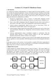
3.3 - Forward Difference - Cont’d
u
u i+1
Predicted du/dx
u i
True du/dx
u i-1
∆x ∆x
∂f
∂x ≈ f i+1 − f i
. (3.7 F&P )
∆x
Truncation Error:
T.E. ∼ O(∆x).
x i-1
x i
x i+1
x
17

3.3 - Backward Difference: ∂f
∂x
By expanding f i−1 about the point x i .
f i−1 = f i − ∆x
( ) ∂f
∂x
i
+ 1 2! ∆x2 ( ∂ 2 f
∂x 2 )i
− 1 3! ∆x3 ( ∂ 3 f
∂x 3 )i
+ H.
18

3.3 - Backward Difference: ∂f
∂x
By expanding f i−1 about the point x i .
f i−1 = f i − ∆x
( ) ∂f
∂x
i
+ 1 2! ∆x2 ( ∂ 2 f
∂x 2 )i
− 1 3! ∆x3 ( ∂ 3 f
∂x 3 )i
+ H.
Similarly, rearranging the above Eqn. (3.3) and dividing by
the finite-difference ∆x gives
∂f
∂x = f i − u i−1
∆x
+ 1 2!
∂ 2 f
∂x 2 ∆x − 1 3!
∂ 3 f
∂x 3 ∆x2 + H. (3.5 F&P )
The first term is a Finite Difference Approximation.
The next term is the Leading Error term: O(∆x).
18

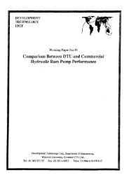
3.3 - Backward Difference - Cont’d
Formula (3.5) is usually recast in the following form
∂f
∂x = f i − f i−1
∆x
+ O(∆x). (3.8 FP )
This is referred to as the first-order backward
difference.
u
u i+1
u i
True du/dx
Predicted du/dx
u i-1
∂f
∂x ≈ f i − f i−1
. (3.8 F&P )
∆x
Truncation Error:
T.E. ∼ O(∆x).
∆x
∆x
x i-1
x i
x i+1
x
19

3.3 - Central Difference: ∂f
∂x
Taylor Series of f i+1 & f i−1 at both x i+1 & x i−1 .
( ) ∂f
f i+1 = f i + ∆x + 1 ( ∂ 2 f
∂x
i
2! ∆x2 ∂x
)i
2 ( ) ∂f
f i−1 = f i − ∆x + 1 ( ∂ 2 f
∂x
i
2! ∆x2 ∂x
)i
2
+ 1 3! ∆x3 ( ∂ 3 f
∂x 3 )i
− 1 3! ∆x3 ( ∂ 3 f
∂x 3 )i
+ H,
+ H.
20

3.3 - Central Difference: ∂f
∂x
Taylor Series of f i+1 & f i−1 at both x i+1 & x i−1 .
( ) ∂f
f i+1 = f i + ∆x + 1 ( ∂ 2 f
∂x
i
2! ∆x2 ∂x
)i
2 ( ) ∂f
f i−1 = f i − ∆x + 1 ( ∂ 2 f
∂x
i
2! ∆x2 ∂x
)i
2
+ 1 3! ∆x3 ( ∂ 3 f
∂x 3 )i
− 1 3! ∆x3 ( ∂ 3 f
∂x 3 )i
+ H,
+ H.
The widely used central difference formula can be
obtained from subtraction of two Taylor series expansions.
∂f
∂x = f i+1 − f i−1
2∆x
− 1 3!
∂ 3 f
∂x 3 ∆x2 − 1 5!
∂ 5 f
∂x 5 ∆x4 + H. (3.6 F&P )
20

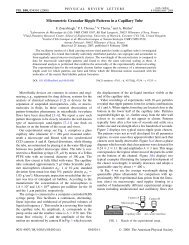
3.3 - Central Differences - Cont’d
Formula (3.6) is usually recast in the following form
∂f
∂x = f i+1 − f i−1
2∆x
+ O(∆x 2 ). (3.8 FP )
This is a second-order formula.
u
u i+1
Predicted du/dx
u i
True du/dx
u i-1
∆x ∆x
∂f
∂x ≈ f i+1 − f i−1
. (3.8 F&P )
2∆x
Truncation Error:
T.E. ∼ O(∆x 2 ).
x i-1
x i
x i+1
x
21

3.3 - Truncation Errors
Numerically evaluated at x = 4.
The absolute values of the differences from the exact
solution.
f(x) = sin x
x 3 .
With ∆x = 0.1
f i−1 = −0.0115943,
f i = −0.0118250,
f i+1 = −0.0118726.
22

3.3 - Fourth Order Accuracy
In general, we can obtain higher accuracy if we include
more points.
Fourth Order Accuracy: T.E. ∼ O(∆x 4 ).
23

3.3 - Fourth Order Accuracy
In general, we can obtain higher accuracy if we include
more points.
Fourth Order Accuracy: T.E. ∼ O(∆x 4 ).
Taylor Series of f i+2 , f i+1 , f i−1 & f i−2 at x i+2 , x i+1 , x i−1 &
x i−2 .
( ) ∂f
f i+2 = f i + 2∆x + 1 ( ∂ 2 )
f
∂x 2! (2∆x)2 ∂x 2
( ) ∂f
f i+1 = f i + ∆x + 1 ( ∂ 2 )
f
∂x 2! ∆x2 ∂x 2
( ) ∂f
f i−1 = f i − ∆x + 1 ( ∂ 2 )
f
∂x 2! ∆x2 ∂x 2
( ) ∂f
f i−2 = f i − 2∆x + 1 ( ∂ 2 )
f
∂x 2! (2∆x)2 ∂x 2
+ 1 3! (2∆x)3 ( ∂ 3 f
∂x 3 )
+ 1 3! ∆x3 ( ∂ 3 f
∂x 3 )
− 1 3! ∆x3 ( ∂ 3 f
∂x 3 )
+ H,
+ H,
− 1 3! (2∆x)3 ( ∂ 3 f
∂x 3 )
+ H,
+ H.
23

3.3 - Fourth Order Accuracy - Cont’d
Rearranging the above equations and dividing by the
finite-difference ∆x gives
∂f
∂x = −f i+2 + 8f i+1 − 8f i−1 + f i−2
12∆x
∂f
∂x = −f i+2 + 8f i+1 − 8f i−1 + f i−2
12∆x
+ 4 5!
∂ 5 f
∂x 5 ∆x4 + H.
+ O(∆x 4 ). (3.14 F&P )
24

3.3 - Fourth Order Accuracy - Cont’d
Rearranging the above equations and dividing by the
finite-difference ∆x gives
∂f
∂x = −f i+2 + 8f i+1 − 8f i−1 + f i−2
12∆x
∂f
∂x = −f i+2 + 8f i+1 − 8f i−1 + f i−2
12∆x
+ 4 5!
∂ 5 f
∂x 5 ∆x4 + H.
+ O(∆x 4 ). (3.14 F&P )
Fourth Order Accuracy: T.E. ∼ O(∆x 4 ).
Requires four grid points to achieve the fourth order
accuracy.
24

3.3 - Fourth Order Accuracy - Cont’d
Rearranging the above equations and dividing by the
finite-difference ∆x gives
∂f
∂x = −f i+2 + 8f i+1 − 8f i−1 + f i−2
12∆x
∂f
∂x = −f i+2 + 8f i+1 − 8f i−1 + f i−2
12∆x
+ 4 5!
∂ 5 f
∂x 5 ∆x4 + H.
+ O(∆x 4 ). (3.14 F&P )
Fourth Order Accuracy: T.E. ∼ O(∆x 4 ).
Requires four grid points to achieve the fourth order
accuracy.
24

3.3 - Higher Order Accuracy
Second-Order Accuracy: T.E. ∼ O(∆x 2 ).
Requires Two grid points, x i+1 & x i−1 .
∂f
∂x = f i+1 − f i−1
2∆x
+ O(∆x 2 ). (3.9 FP )
25

3.3 - Higher Order Accuracy
Second-Order Accuracy: T.E. ∼ O(∆x 2 ).
Requires Two grid points, x i+1 & x i−1 .
∂f
∂x = f i+1 − f i−1
2∆x
+ O(∆x 2 ). (3.9 FP )
Fourth-Order Accuracy: T.E. ∼ O(∆x 4 ).
Requires Four grid points at x i+2 , x i+1 , x i−1 & x i−2 .
∂f
∂x = −f i+2 + 8f i+1 − 8f i−1 + f i−2
12∆x
+ O(∆x 4 ). (3.14 F&P )
25

3.3 - Higher Order Accuracy
Second-Order Accuracy: T.E. ∼ O(∆x 2 ).
Requires Two grid points, x i+1 & x i−1 .
∂f
∂x = f i+1 − f i−1
2∆x
+ O(∆x 2 ). (3.9 FP )
Fourth-Order Accuracy: T.E. ∼ O(∆x 4 ).
Requires Four grid points at x i+2 , x i+1 , x i−1 & x i−2 .
∂f
∂x = −f i+2 + 8f i+1 − 8f i−1 + f i−2
12∆x
+ O(∆x 4 ). (3.14 F&P )
N-th Order Accuracy: T.E. ∼ O(∆x N ).
Requires N grid points to achieve the N-th order
accuracy.
Taylor Series of f i+N/2 , . . . , f i+1 , f i−1 , . . . & f i−N/2 . 25

3.3 - High Order Accuracy - Cont’d
N-th Order Accuracy: T.E. ∼ O(∆x N ).
Requires N grid points to achieve the N-th order
accuracy.
The main difficulty with the higher order formulae occurs
near boundaries of the domain.
For example, the derivative of f at x 1 would require the
value of f at x −1 which is not available.
In practice, to alleviate this problem, we utilise lower
order or non-central formulae near boundaries.
26

3.3 - High Order Accuracy - Cont’d
N-th Order Accuracy: T.E. ∼ O(∆x N ).
Requires N grid points to achieve the N-th order
accuracy.
The main difficulty with the higher order formulae occurs
near boundaries of the domain.
For example, the derivative of f at x 1 would require the
value of f at x −1 which is not available.
In practice, to alleviate this problem, we utilise lower
order or non-central formulae near boundaries.
26

3.3 - High Order Accuracy - Cont’d
N-th Order Accuracy: T.E. ∼ O(∆x N ).
Requires N grid points to achieve the N-th order
accuracy.
The main difficulty with the higher order formulae occurs
near boundaries of the domain.
For example, the derivative of f at x 1 would require the
value of f at x −1 which is not available.
In practice, to alleviate this problem, we utilise lower
order or non-central formulae near boundaries.
26

3.4 Second Order Derivative: ∂2 f
∂x 2
Similar formulae can be derived for second order or higher
order derivatives.
( ) ∂f
f i+1 = f i + ∆x
∂x
( ) ∂f
f i−1 = f i − ∆x
∂x
i
i
+ 1 ( ∂ 2 f
2! ∆x2 ∂x
)i
2
+ 1 ( ∂ 2 f
2! ∆x2 ∂x
)i
2
+ 1 3! ∆x3 ( ∂ 3 f
∂x 3 )i
− 1 3! ∆x3 ( ∂ 3 f
∂x 3 )i
+ H,
+ H.
27

3.4 Second Order Derivative: ∂2 f
∂x 2
Similar formulae can be derived for second order or higher
order derivatives.
( ) ∂f
f i+1 = f i + ∆x
∂x
( ) ∂f
f i−1 = f i − ∆x
∂x
i
+ 1 ( ∂ 2 f
2! ∆x2 ∂x
)i
2
+ 1 ( ∂ 2 f
2! ∆x2 ∂x
)i
2
After minor rearrangement, we get
i
+ 1 3! ∆x3 ( ∂ 3 f
∂x 3 )i
− 1 3! ∆x3 ( ∂ 3 f
∂x 3 )i
+ H,
+ H.
∂ 2 f
∂x 2 = f i+1 − 2f i + f i−1
∆x 2
+ 1 12 ∆x2∂4 f
∂x 4 + H. (3.30FP )
27

3.4 - Higher Order Accuracy: O(∆x 4 )
Second Order Accuracy: O(∆x 2 )
∂ 2 f
∂x 2 = f i+1 − 2f i + f i−1
∆x 2 + O(∆x 2 ). (3.30 FP )
28

3.4 - Higher Order Accuracy: O(∆x 4 )
Second Order Accuracy: O(∆x 2 )
∂ 2 f
∂x 2 = f i+1 − 2f i + f i−1
∆x 2 + O(∆x 2 ). (3.30 FP )
Fourth Order Accuracy: O(∆x 4 )
∂ 2 f
∂x 2 = −f i+2 + 16f i+1 − 30f i + 16f i−1 − f i−2
12∆x 2 + O(∆x 4 ).
(3.32 F&P )
Taylor Series of f i+N/2 , . . . , f i+1 , f i−1 , . . . & f i−N/2 at N
points.
28

3.4 Third Order Derivative: ∂3 f
∂x 3
Similar formulae can be derived for higher order derivatives.
( ) ∂f
f i+1 = f i + ∆x + 1 ( ∂ 2 f
∂x
i
2! ∆x2 ∂x
)i
2 + 1 ( ∂ 3 f
3! ∆x3 ∂x
)i
3 + H,
( ) ∂f
f i−1 = f i − ∆x + 1 ( ∂ 2 f
∂x
i
2! ∆x2 ∂x
)i
2 − 1 ( ∂ 3 f
3! ∆x3 ∂x
)i
3 + H.
29

3.4 Third Order Derivative: ∂3 f
∂x 3
Similar formulae can be derived for higher order derivatives.
( ) ∂f
f i+1 = f i + ∆x + 1 ( ∂ 2 f
∂x
i
2! ∆x2 ∂x
)i
2 + 1 ( ∂ 3 f
3! ∆x3 ∂x
)i
3 + H,
( ) ∂f
f i−1 = f i − ∆x + 1 ( ∂ 2 f
∂x
i
2! ∆x2 ∂x
)i
2 − 1 ( ∂ 3 f
3! ∆x3 ∂x
)i
3 + H.
Second Order Accuracy
∂ 3 f
∂x 3 = f i+2 − 2f i+1 + 2f i−1 − f i−2
2∆x 3 + O(∆x 2 ).
29

3.4 Third Order Derivative: ∂3 f
∂x 3
Similar formulae can be derived for higher order derivatives.
( ) ∂f
f i+1 = f i + ∆x + 1 ( ∂ 2 f
∂x
i
2! ∆x2 ∂x
)i
2 + 1 ( ∂ 3 f
3! ∆x3 ∂x
)i
3 + H,
( ) ∂f
f i−1 = f i − ∆x + 1 ( ∂ 2 f
∂x
i
2! ∆x2 ∂x
)i
2 − 1 ( ∂ 3 f
3! ∆x3 ∂x
)i
3 + H.
Second Order Accuracy
∂ 3 f
∂x 3 = f i+2 − 2f i+1 + 2f i−1 − f i−2
2∆x 3 + O(∆x 2 ).
Fourth Order Accuracy
∂ 3 f
∂x 3 = −f i+3 + 8f i+2 − 13f i+1 + 13f i−1 − 8f i−2 + f i−3
8∆x 3 + O(∆x 4 ).
29

First Order Accuracy: O(∆x)
FORWARD & BACKWARD DIFFERENCES
30

First Order Accuracy: O(∆x)
FORWARD & BACKWARD DIFFERENCES
Forward Difference
∂f
∂x = f i+1 − f i
∆x
+ O(∆x). (3.7 FP )
30

First Order Accuracy: O(∆x)
FORWARD & BACKWARD DIFFERENCES
Forward Difference
∂f
∂x = f i+1 − f i
∆x
+ O(∆x). (3.7 FP )
Backward Difference
∂f
∂x = f i − f i−1
∆x
+ O(∆x). (3.8 FP )
30

Second Order Accuracy: O(∆x 2 )
CENTRAL DIFFERENCES
31

Second Order Accuracy: O(∆x 2 )
CENTRAL DIFFERENCES
First Derivative
∂f
∂x = f i+1 − f i−1
2∆x
+ O(∆x 2 ). (3.9 FP )
31

Second Order Accuracy: O(∆x 2 )
CENTRAL DIFFERENCES
First Derivative
∂f
∂x = f i+1 − f i−1
2∆x
+ O(∆x 2 ). (3.9 FP )
Second Derivative
∂ 2 f
∂x 2 = f i+1 − 2f i + f i−1
∆x 2 + O(∆x 2 ). (3.30 FP )
31

Second Order Accuracy: O(∆x 2 )
CENTRAL DIFFERENCES
First Derivative
∂f
∂x = f i+1 − f i−1
2∆x
+ O(∆x 2 ). (3.9 FP )
Second Derivative
Third Derivative
∂ 2 f
∂x 2 = f i+1 − 2f i + f i−1
∆x 2 + O(∆x 2 ). (3.30 FP )
∂ 3 f
∂x 3 = f i+2 − 2f i+1 + 2f i−1 − f i−2
2∆x 3 + O(∆x 2 ).
31

Fourth Order Accuracy: O(∆x 4 )
CENTRAL DIFFERENCES
32

Fourth Order Accuracy: O(∆x 4 )
CENTRAL DIFFERENCES
First Derivative
∂f
∂x = −f i+2 + 8f i+1 − 8f i−1 + f i−2
12∆x
+ O(∆x 4 ). (3.14 F&P )
32

Fourth Order Accuracy: O(∆x 4 )
CENTRAL DIFFERENCES
First Derivative
∂f
∂x = −f i+2 + 8f i+1 − 8f i−1 + f i−2
12∆x
+ O(∆x 4 ). (3.14 F&P )
Second Derivative
∂ 2 f
∂x 2 = −f i+2 + 16f i+1 − 30f i + 16f i−1 − f i−2
12∆x 2 + O(∆x 4 ).
(3.32 F&P )
32

Fourth Order Accuracy: O(∆x 4 )
CENTRAL DIFFERENCES
First Derivative
∂f
∂x = −f i+2 + 8f i+1 − 8f i−1 + f i−2
12∆x
+ O(∆x 4 ). (3.14 F&P )
Second Derivative
∂ 2 f
∂x 2 = −f i+2 + 16f i+1 − 30f i + 16f i−1 − f i−2
12∆x 2 + O(∆x 4 ).
Third Derivative
(3.32 F&P )
∂ 3 f
∂x 3 = −f i+3 + 8f i+2 − 13f i+1 + 13f i−1 − 8f i−2 + f i−3
8∆x 3 + O(∆x 4 ).
32

Finite Difference Method for Elliptic PDE
Elliptic PDE: Laplace equation
∂ 2 u
∂x 2 + ∂2 u
∂y 2 = f(x, y). 33

Finite Difference Method for Elliptic PDE
Elliptic PDE: Laplace equation
∂ 2 u
∂x 2 + ∂2 u
= f(x, y).
∂y2 FDM: Using Central Differences with Second Order
Accuracy
∂ 2 u
∂x 2 = u i+1 − 2u i + u i−1
∆x 2 + O(∆x 2 ),
∂ 2 u
∂y 2 = u j+1 − 2u j + u j−1
∆y 2 + O(∆y 2 ). (3.30 FP )
33

Finite Difference Method for Elliptic PDE
Elliptic PDE: Laplace equation
∂ 2 u
∂x 2 + ∂2 u
= f(x, y).
∂y2 FDM: Using Central Differences with Second Order
Accuracy
∂ 2 u
∂x 2 = u i+1 − 2u i + u i−1
∆x 2 + O(∆x 2 ),
∂ 2 u
∂y 2 = u j+1 − 2u j + u j−1
∆y 2 + O(∆y 2 ). (3.30 FP )
Resulting Finite Difference Equation (FDE) is
u i+1,j − 2u i,j + u i−1,j
∆x 2
+ u i,j+1 − 2u i,j + u i,j−1
∆y 2 = f i,j .
33

One-Dimensional FDM
Elliptic PDE: Laplace equation
∂ 2 u
∂x 2 = f(x). 34

One-Dimensional FDM
Elliptic PDE: Laplace equation
∂ 2 u
∂x 2 = f(x).
Using Central Differences with Second Order Accuracy
u i+1 − 2u i + u i−1
∆x 2 = g i .
34

One-Dimensional FDM
Elliptic PDE: Laplace equation
∂ 2 u
∂x 2 = f(x).
Using Central Differences with Second Order Accuracy
u i+1 − 2u i + u i−1
∆x 2 = g i .
Multiplying ∆x 2 & rearranging, FDE is
u i−1 − 2u i + u i+1 = f i .
where α = 1
∆x 2 & f i = g i /α.
34

One-Dimensional FDM
Elliptic PDE: Laplace equation
∂ 2 u
∂x 2 = f(x).
Using Central Differences with Second Order Accuracy
u i+1 − 2u i + u i−1
∆x 2 = g i .
Multiplying ∆x 2 & rearranging, FDE is
u i−1 − 2u i + u i+1 = f i .
where α = 1
∆x 2 & f i = g i /α.
34

One-Dimensional FDM
∂ 2 u
∂x 2 = f(x).
Divide the computational
domain into NX steps
(control volumes).
∆x
1 2 i i+1 NX NX+1
u i−1 − 2u i + u i+1 = f i .
35

One-Dimensional FDM
∂ 2 u
∂x 2 = f(x).
Divide the computational
domain into NX steps
(control volumes).
Apply the FDE to the
interior points
∆x
1 2 i i+1 NX NX+1
x 2 , x 3 , . . . , x i , . . . , x NX .
x 1 & x NX+1 are
boundary points.
u i−1 − 2u i + u i+1 = f i .
35

One-Dimensional FDM
∂ 2 u
∂x 2 = f(x).
Divide the computational
domain into NX steps
(control volumes).
Apply the FDE to the
interior points
∆x
1 2 i i+1 NX NX+1
x 2 , x 3 , . . . , x i , . . . , x NX .
x 1 & x NX+1 are
boundary points.
Domain size L = 1 &
∆x = 0.2
u i−1 − 2u i + u i+1 = f i .
x 1 , x 2 , x 3 , x 4 , x 5 , x 6 .
x 1 & x 6 are boundary.
35

3.8 Algebraic Equation System
u 1 − 2u 2 + u 3 = f 2
u 2 − 2u 3 + u 4 = f 3 ,
.
u i−1 − 2u i + u i+1 = f i ,
.
u NX−2 − 2u NX−1 + u NX = f NX−1 ,
u NX−1 − 2u NX + u NX+1 = f NX .
Here, NX is the number of ∆x and we have NX −1 number
of equations for u 2 , u 3 , u 4 , . . . u i , . . . , u NX−2 , u NX−1 , u NX .
u 1 and u NX+1 are boundary values.
36

3.8 - Linear Algebraic Equation
Finite Difference Equations, (FDE) are
u i−1 − 2u i + u i+1 = f i .
37

3.8 - Linear Algebraic Equation
Finite Difference Equations, (FDE) are
u i−1 − 2u i + u i+1 = f i .
The result of discretisation is a system of linear algebraic
equations:
A P φ P + ∑ l
A l φ l = Q P , (3.42 F&P )
P denotes the node at which the FDE is approximated,
Index l runs over the neighbour nodes involved in FDA.
37

3.8 - Matrix Equations for 1D FDM
The result of discretisation is a system of linear algebraic
equations:
⎛
⎞⎛
−2 1
1 −2 1
1 −2 1
⎜
⎝ 1 −2 1 ⎟⎜
⎠⎝
1 −2
u 2
u 3
u i
u NX−1
u NX
⎞ ⎛
⎞
f 2 − u 1
f 3
=
f i
.
⎟ ⎜
⎠ ⎝ f NX−1
⎟
⎠
f NX − u NX+1
38

3.8 - Matrix Equations - Cont’d
Algebraic Equation:
Aφ = Q. (3.43 F&P )
39

3.8 - Matrix Equations - Cont’d
Algebraic Equation:
Aφ = Q. (3.43 F&P )
A =
⎛
⎜
⎝
−2 1
1 −2 1
1 −2 1
1 −2 1
1 −2
⎞
,
⎟
⎠
39

3.8 - Matrix Equations - Cont’d
Algebraic Equation:
Aφ = Q. (3.43 F&P )
A =
⎛
⎜
⎝
−2 1
1 −2 1
1 −2 1
1 −2 1
1 −2
⎞
,Q =
⎟
⎠
⎛
⎜
⎝
⎞
f 2 − u 1
f 3
f i
,
f NX−1
⎟
⎠
f NX − u NX+1
39

3.8 - Matrix Equations - Cont’d
Algebraic Equation:
Aφ = Q. (3.43 F&P )
A =
⎛
⎜
⎝
−2 1
1 −2 1
1 −2 1
1 −2 1
1 −2
⎞
,Q =
⎟
⎠
⎛
⎜
⎝
⎞
f 2 − u 1
f 3
f i
,
f NX−1
⎟
⎠
f NX − u NX+1
and φ = (u 2 , u 3 , . . . , u i , . . . u NX−1 , u NX ) T .
39

1-D Navier-Stokes Equation
Elliptic PDE: Laplace equation
1
Re
∂ 2 u
∂y 2 = dp
dx . 40

1-D Navier-Stokes Equation
Elliptic PDE: Laplace equation
1
Re
∂ 2 u
∂y 2 = dp
dx .
Using Central Differences with Second Order Accuracy
1
Re
u j+1 − 2u j + u j−1
∆y 2
= dp
dx . 40

1-D Navier-Stokes Equation
Elliptic PDE: Laplace equation
1
Re
∂ 2 u
∂y 2 = dp
dx .
Using Central Differences with Second Order Accuracy
1
Re
u j+1 − 2u j + u j−1
∆y 2
= dp
dx .
Multiplying Re∆y 2 & rearranging, FDE is
u j−1 − 2u j + u j+1 = dp
dx Re/α.
where α = 1
∆y 2 . 40

One-Dimensional FDM
1
Re
∂ 2 u
∂y 2 = dp
dx .
Divide the computational
domain into NX steps
(control volumes).
∆x
1 2 i i+1 NX NX+1
u j−1 − 2u j + u j+1 = dp
dx Re/α.
41

One-Dimensional FDM
1
Re
∂ 2 u
∂y 2 = dp
dx .
Divide the computational
domain into NX steps
(control volumes).
Apply the FDE to the
interior points
x 2 , x 3 , . . . , x i , . . . , x NX .
∆x
1 2 i i+1 NX NX+1
x 1 & x NX+1 are
boundary points.
u j−1 − 2u j + u j+1 = dp
dx Re/α.
41

One-Dimensional FDM
1
Re
∂ 2 u
∂y 2 = dp
dx .
Divide the computational
domain into NX steps
(control volumes).
Apply the FDE to the
interior points
x 2 , x 3 , . . . , x i , . . . , x NX .
∆x
1 2 i i+1 NX NX+1
x 1 & x NX+1 are
boundary points.
Domain size L = 1.2 &
∆x = 0.2
u j−1 − 2u j + u j+1 = dp
dx Re/α.
x 1 , x 2 , x 3 , x 4 , x 5 , x 6 x 7 .
x 1 & x 7 are boundary.
41

3.8 Algebraic Equation System
u 1 − 2u 2 + u 3 = f 2 /α,
u 2 − 2u 3 + u 4 = f 3 /α,
u 3 − 2u 4 + u 5 = f 4 /α,
u 4 − 2u 5 + u 6 = f 5 /α,
u 5 − 2u 6 + u 7 = f 6 /α.
Here, NY = 6 is the number of ∆y = 0.2 and we have
NY − 1 = 5 number of equations for u 2 , u 3 , u 4 , u 5 , u 6 .
u 1 and u 7 are boundary values.
f = Re
α . 42

3.8 - Matrix Equations for 1D FDM
The result of discretisation is a system of linear algebraic
equations:
⎛
⎞⎛
−2 1
1 −2 1
1 −2 1
⎜
⎝ 1 −2 1 ⎟⎜
⎠⎝
1 −2
⎞ ⎛
u 2
u 3
u 4
=
u 5
⎟ ⎜
⎠ ⎝
u 6
⎞
f2/α − u 1
f3/α
f 4 /α
.
f 5 /α ⎟
⎠
f 6 /α − u 7
43

3.8 - Matrix Equations for 1D FDM
The result of discretisation is a system of linear algebraic
equations:
⎛
⎞⎛
−2 1
1 −2 1
1 −2 1
⎜
⎝ 1 −2 1 ⎟⎜
⎠⎝
1 −2
⎞ ⎛
u 2
u 3
u 4
=
u 5
⎟ ⎜
⎠ ⎝
u 6
⎞
f2/α − u 1
f3/α
f 4 /α
.
f 5 /α ⎟
⎠
f 6 /α − u 7
At walls, due to no-slip boundary condition, u 1 = 0 & u 7 = 0.
43

Tri-Diagonal Matrix
A =
⎛
⎜
⎝
AX = B
⎞
b 1 c 1
a 2 b 2 c 2
a 3 b 3 c 3
,B =
a NX−1 b NX−1 c NX−1
⎟
⎠
a NX b NX
⎛
⎜
⎝
f 1
f 2
f 3
f NX−1
f NX
⎞
,
⎟
⎠
X = (u 1 , u 2 , u 3 , u NX−1 , u NX ) T .
44

TDMA: Thomas Algorithm
An upper triangular form of the tridiagonal matrix may be
obtained by computing the new b i by
b i = b i −
and the new f i by
f i = f i −
a i
b i−1
c i−1 ,
a i
b i−1
f i−1 ,
i = 2,3, . . . , NX,
i = 2,3, . . . , NX,
then computing the unknowns from back substitution according
to u NX = f NX /b NX and then
u k = f k − c k u k+1
b k
, k = NX − 1, NX − 2, . . . ,2,1.
45

3.8 - Matrix Equations - Cont’d
Algebraic Equation:
Aφ = Q. (3.43 F&P )
46

3.8 - Matrix Equations - Cont’d
Algebraic Equation:
Aφ = Q. (3.43 F&P )
A =
⎛
⎜
⎝
−2 1
1 −2 1
1 −2 1
1 −2 1
1 −2
⎞
,
⎟
⎠
46

3.8 - Matrix Equations - Cont’d
Algebraic Equation:
Aφ = Q. (3.43 F&P )
A =
⎛
⎜
⎝
−2 1
1 −2 1
1 −2 1
1 −2 1
1 −2
⎞
,Q =
⎟
⎠
⎛
⎜
⎝
⎞
f2/α − u 1
f3/α
f4/α
,
f5/α ⎟
⎠
f6/α − u 7
46

3.8 - Matrix Equations - Cont’d
Algebraic Equation:
Aφ = Q. (3.43 F&P )
A =
⎛
⎜
⎝
−2 1
1 −2 1
1 −2 1
1 −2 1
1 −2
⎞
,Q =
⎟
⎠
⎛
⎜
⎝
⎞
f2/α − u 1
f3/α
f4/α
,
f5/α ⎟
⎠
f6/α − u 7
and φ = (u 2 , u 3 , u 4 , u 5 , u 6 ) T .
46

Solution to 1D Matrix Equations
Direct solver using Gauss elimination.
47

Solution to 1D Matrix Equations
Direct solver using Gauss elimination.
Tri-Diagonal Matrix Algorithm.
47

Solution to 1D Matrix Equations
Direct solver using Gauss elimination.
Tri-Diagonal Matrix Algorithm.
More details on Martix Computation (Ch. 5)
47

Example of First-Order ODE
Heat Tranfer for Conduction:
d 2 T
dx 2 + h′ (T a − T) = 0
Computational domain: 0 ≤ x ≤ 10.
T 1 = 40, T NX = 200, T a = 20 & h ′ = 0.01.
48

Example of First-Order ODE
Heat Tranfer for Conduction:
d 2 T
dx 2 + h′ (T a − T) = 0
Computational domain: 0 ≤ x ≤ 10.
T 1 = 40, T NX = 200, T a = 20 & h ′ = 0.01.
Using the second-order central difference
T i+1 − 2T i + T i−1
∆x 2 − h ′ T i = −h ′ T a ,
( )
1 2
∆x 2T i−1 −
∆x 2 + h′ T i + 1
∆x 2u i+1 = −h ′ T a .
48

3.11 Example
The generic transport equation is.
∂ρu j φ
∂x j
= ∂
∂x j
(
Γ ∂φ
∂x j
)
+ q φ . (3.1 F&P )
49

3.11 Example
The generic transport equation is.
∂ρu j φ
∂x j
= ∂
∂x j
(
Γ ∂φ
∂x j
)
+ q φ . (3.1 F&P )
A one-dimensional generic transport equation is.
∂ρuφ
∂x = ∂ (
Γ ∂φ )
. (3.1 F&P )
∂x ∂x
With the boundary conditions: φ = φ 0 at x = 0, φ = φ L at
x = L.
The density ρ and the velocity u are assumed constant.
49