Chapter 5 â Sequential Circuits
Chapter 5 â Sequential Circuits
Chapter 5 â Sequential Circuits

You also want an ePaper? Increase the reach of your titles
YUMPU automatically turns print PDFs into web optimized ePapers that Google loves.
Logic and Computer Design Fundamentals<br />
<strong>Chapter</strong> 5 – <strong>Sequential</strong><br />
<strong>Circuits</strong><br />
Part 2 – <strong>Sequential</strong> Circuit Design<br />
Charles Kime & Thomas Kaminski<br />
© 2008 Pearson Education, Inc.<br />
(Hyperlinks are active in View Show mode)<br />
Overview<br />
• Part 1 - Storage Elements and <strong>Sequential</strong><br />
Circuit Analysis<br />
• Part 2- <strong>Sequential</strong> Circuit Design<br />
• Specification<br />
• Formulation<br />
• State Assignment<br />
• Flip-Flop Input and Output Equation<br />
Determination<br />
• Verification<br />
• Part 3 – State Machine Design<br />
<strong>Chapter</strong> 5 - Part 2 2<br />
1
The Design Procedure<br />
• Specification<br />
• Formulation - Obtain a state diagram or state table<br />
• State Assignment - Assign binary codes to the states<br />
• Flip-Flop Input Equation Determination - Select flip-flop<br />
types and derive flip-flop equations from next state entries in the<br />
table<br />
• Output Equation Determination - Derive output equations<br />
from output entries in the table<br />
• Optimization - Optimize the equations<br />
• Technology Mapping - Find circuit from equations and map to<br />
flip-flops and gate technology<br />
• Verification - Verify correctness of final design<br />
<strong>Chapter</strong> 5 - Part 2 3<br />
Specification<br />
• Component Forms of Specification<br />
• Written description<br />
• Mathematical description<br />
• Hardware description language*<br />
• Tabular description*<br />
• Equation description*<br />
• Diagram describing operation (not just structure)*<br />
• Relation to Formulation<br />
• If a specification is rigorous at the binary level<br />
(marked with * above), then all or part of<br />
formulation may be completed<br />
<strong>Chapter</strong> 5 - Part 2 4<br />
2
Formulation: Finding a State Diagram<br />
• A state is an abstraction of the history of the past<br />
applied inputs to the circuit (including power-up reset<br />
or system reset).<br />
• The interpretation of “past inputs” is tied to the synchronous<br />
operation of the circuit. E. g., an input value (other than an<br />
asynchronous reset) is measured only during the setup-hold<br />
time interval for an edge-triggered flip-flop.<br />
• Examples:<br />
• State A represents the fact that a 1 input has occurred among<br />
the past inputs.<br />
• State B represents the fact that a 0 followed by a 1 have<br />
occurred as the most recent past two inputs.<br />
<strong>Chapter</strong> 5 - Part 2 5<br />
Formulation: Finding a State Diagram<br />
• In specifying a circuit, we use states to remember<br />
meaningful properties of past input sequences that are<br />
essential to predicting future output values.<br />
• A sequence recognizer is a sequential circuit that<br />
produces a distinct output value whenever a prescribed<br />
pattern of input symbols occur in sequence, i.e,<br />
recognizes an input sequence occurence.<br />
• We will develop a procedure specific to sequence<br />
recognizers to convert a problem statement into a state<br />
diagram.<br />
• Next, the state diagram, will be converted to a state<br />
table from which the circuit will be designed.<br />
<strong>Chapter</strong> 5 - Part 2 6<br />
3
Sequence Recognizer Procedure<br />
• To develop a sequence recognizer state diagram:<br />
• Begin in an initial state in which NONE of the initial portion of<br />
the sequence has occurred (typically “reset” state).<br />
• Add a state that recognizes that the first symbol has occurred.<br />
• Add states that recognize each successive symbol occurring.<br />
• The final state represents the input sequence (possibly less the<br />
final input value) occurence.<br />
• Add state transition arcs which specify what happens when a<br />
symbol not in the proper sequence has occurred.<br />
• Add other arcs on non-sequence inputs which transition to<br />
states that represent the input subsequence that has occurred.<br />
• The last step is required because the circuit must recognize the<br />
input sequence regardless of where it occurs within the overall<br />
sequence applied since “reset.”.<br />
<strong>Chapter</strong> 5 - Part 2 7<br />
State Assignment<br />
• Each of the m states must be assigned a<br />
unique code<br />
• Minimum number of bits required is n<br />
such that<br />
n ≥ log 2 m<br />
where x is the smallest integer ≥ x<br />
• There are useful state assignments that<br />
use more than the minimum number of<br />
bits<br />
• There are 2 n - m unused states<br />
<strong>Chapter</strong> 5 - Part 2 8<br />
4
Sequence Recognizer Example<br />
• Example: Recognize the sequence 1101<br />
• Note that the sequence 1111101 contains 1101 and "11" is a<br />
proper sub-sequence of the sequence.<br />
• Thus, the sequential machine must remember that the<br />
first two one's have occurred as it receives another<br />
symbol.<br />
• Also, the sequence 1101101 contains 1101 as both an<br />
initial subsequence and a final subsequence with some<br />
overlap, i. e., 1101101 or 1101101.<br />
• And, the 1 in the middle, 1101101, is in both<br />
subsequences.<br />
• The sequence 1101 must be recognized each time it<br />
occurs in the input sequence.<br />
<strong>Chapter</strong> 5 - Part 2 9<br />
Example: Recognize 1101<br />
• Define states for the sequence to be recognized:<br />
• assuming it starts with first symbol,<br />
• continues through each symbol in the sequence to be<br />
recognized, and<br />
• uses output 1 to mean the full sequence has occurred,<br />
• with output 0 otherwise.<br />
• Starting in the initial state (Arbitrarily named<br />
"A"):<br />
1/0<br />
A B<br />
• Add a state that<br />
recognizes the first "1."<br />
• State "A" is the initial state, and state "B" is the state which<br />
represents the fact that the "first" one in the input<br />
subsequence has occurred. The output symbol "0" means<br />
that the full recognized sequence has not yet occurred.<br />
<strong>Chapter</strong> 5 - Part 2 10<br />
5
Example: Recognize 1101 (continued)<br />
• After one more 1, we have:<br />
• C is the state obtained<br />
when the input sequence<br />
has two "1"s.<br />
• Finally, after 110 and a 1, we have:<br />
A<br />
1/0<br />
B<br />
A<br />
1/0<br />
B<br />
1/0 0/0<br />
C<br />
1/0<br />
D 1/1<br />
C<br />
• Transition arcs are used to denote the output function (Mealy Model)<br />
• Output 1 on the arc from D means the sequence has been recognized<br />
• To what state should the arc from state D go? Remember: 1101101 ?<br />
• Note that D is the last state but the output 1 occurs for the input<br />
applied in D. This is the case when a Mealy model is assumed.<br />
<strong>Chapter</strong> 5 - Part 2 11<br />
Example: Recognize 1101 (continued)<br />
A<br />
1/0<br />
B<br />
1/0 0/0<br />
C<br />
D 1/1<br />
• Clearly the final 1 in the recognized sequence<br />
1101 is a sub-sequence of 1101. It follows a 0<br />
which is not a sub-sequence of 1101. Thus it<br />
should represent the same state reached from the<br />
initial state after a first 1 is observed. We obtain:<br />
A<br />
1/0<br />
B<br />
1/0 0/0<br />
C<br />
D<br />
1/1<br />
<strong>Chapter</strong> 5 - Part 2 12<br />
6
Example: Recognize 1101 (continued)<br />
A<br />
1/0<br />
B<br />
1/0<br />
C<br />
0/0<br />
D<br />
1/1<br />
• The state have the following abstract meanings:<br />
• A: No proper sub-sequence of the sequence has<br />
occurred.<br />
• B: The sub-sequence 1 has occurred.<br />
• C: The sub-sequence 11 has occurred.<br />
• D: The sub-sequence 110 has occurred.<br />
• The 1/1 on the arc from D to B means that the last 1<br />
has occurred and thus, the sequence is recognized.<br />
<strong>Chapter</strong> 5 - Part 2 13<br />
Example: Recognize 1101 (continued)<br />
• The other arcs are added to each state for<br />
inputs not yet listed. Which arcs are missing?<br />
A<br />
1/0<br />
B<br />
1/0<br />
C<br />
0/0<br />
D<br />
• Answer:<br />
1/1<br />
"0" arc from A<br />
"0" arc from B<br />
"1" arc from C<br />
"0" arc from D.<br />
<strong>Chapter</strong> 5 - Part 2 14<br />
7
Example: Recognize 1101 (continued)<br />
• State transition arcs must represent the fact<br />
that an input subsequence has occurred. Thus<br />
we get:<br />
0/0 1/0<br />
A<br />
1/0 1/0<br />
B<br />
C<br />
0/0<br />
D<br />
0/0<br />
1/1<br />
0/0<br />
• Note that the 1 arc from state C to state C<br />
implies that State C means two or more 1's have<br />
occurred.<br />
<strong>Chapter</strong> 5 - Part 2 15<br />
Formulation: Find State Table<br />
• From the State Diagram, we can fill in the State Table.<br />
• There are 4 states, one 0/0<br />
1/0<br />
input, and one output.<br />
We will choose the form<br />
1/0<br />
1/0 0/0<br />
A<br />
B C<br />
with four rows, one for<br />
each current state.<br />
0/0<br />
1/1<br />
• From State A, the 0 and<br />
1 input transitions have<br />
been filled in along with<br />
the outputs.<br />
Present<br />
State<br />
A<br />
B<br />
C<br />
D<br />
0/0<br />
D<br />
Next State<br />
x=0 x=1<br />
Output<br />
x=0 x=1<br />
A B 0 0<br />
<strong>Chapter</strong> 5 - Part 2 16<br />
8
Formulation: Find State Table<br />
• From the state diagram, we complete the<br />
state table.<br />
0/0<br />
1/0<br />
A<br />
1/0<br />
B<br />
1/0<br />
C<br />
0/0<br />
D<br />
Present Next State Output<br />
State x=0 x=1 x=0 x=1<br />
A A B 0 0<br />
B A C 0 0<br />
C D C 0 0<br />
D A B 0 1<br />
• What would the state diagram and state table<br />
look like for the Moore model?<br />
0/0<br />
0/0<br />
1/1<br />
<strong>Chapter</strong> 5 - Part 2 17<br />
Example: Moore Model for Sequence 1101<br />
• For the Moore Model, outputs are associated with<br />
states.<br />
• We need to add a state "E" with output value 1<br />
for the final 1 in the recognized input sequence.<br />
• This new state E, though similar to B, would generate<br />
an output of 1 and thus be different from B.<br />
• The Moore model for a sequence recognizer<br />
usually has more states than the Mealy model.<br />
<strong>Chapter</strong> 5 - Part 2 18<br />
9
Example: Moore Model (continued)<br />
• We mark outputs on<br />
states for Moore model<br />
1 1<br />
0<br />
• Arcs now show only<br />
state transitions<br />
• Add a new state E to<br />
0 1<br />
1<br />
produce the output 1<br />
• Note that the new state,<br />
0 E/1<br />
E produces the same behavior 0<br />
in the future as state B. But it gives a different output<br />
at the present time. Thus these states do represent a<br />
different abstraction of the input history.<br />
0<br />
A/0 B/0 C/0 D/0<br />
1<br />
<strong>Chapter</strong> 5 - Part 2 19<br />
Example: Moore Model (continued)<br />
• The state table is shown<br />
below<br />
• Memory aid re more<br />
state in the Moore model:<br />
“Moore is More.”<br />
0<br />
1<br />
A/0<br />
1<br />
B/0<br />
1 0<br />
C/0 D/0<br />
0 1<br />
1<br />
0 E/1<br />
Present<br />
State<br />
Next State<br />
x=0 x=1<br />
A A B 0<br />
B A C 0<br />
C D C 0<br />
D A E 0<br />
E A C 1<br />
Output<br />
y<br />
0<br />
<strong>Chapter</strong> 5 - Part 2 20<br />
10
State Assignment – Example 1<br />
Present Next State Output<br />
State x=0 x=1 x=0 x=1<br />
A A B 0 0<br />
B A B 0 1<br />
• How may assignments of codes with a<br />
minimum number of bits?<br />
• Two – A = 0, B = 1 or A = 1, B = 0<br />
• Does it make a difference?<br />
• Only in variable inversion, so small, if any.<br />
<strong>Chapter</strong> 5 - Part 2 21<br />
State Assignment – Example 2<br />
Present Next State Output<br />
State x=0 x=1 x=0 x=1<br />
A A B 0 0<br />
B A C 0 0<br />
C D C 0 0<br />
D A B 0 1<br />
• How may assignments of codes with a<br />
minimum number of bits?<br />
• 4 × 3 × 2 × 1 = 24<br />
• Does code assignment make a difference in<br />
cost?<br />
<strong>Chapter</strong> 5 - Part 2 22<br />
11
State Assignment – Example 2 (continued)<br />
• Counting Order Assignment: A = 0 0, B = 0 1,<br />
C = 1 0, D = 1 1<br />
• The resulting coded state table:<br />
Present<br />
State<br />
Next State<br />
x = 0 x = 1<br />
Output<br />
x = 0 x = 1<br />
0 0<br />
0 0<br />
0 1<br />
0<br />
0<br />
0 1<br />
0 0<br />
1 0<br />
0<br />
0<br />
1 0<br />
1 1<br />
1 0<br />
0<br />
0<br />
1 1<br />
0 0<br />
0 1<br />
0<br />
1<br />
<strong>Chapter</strong> 5 - Part 2 23<br />
State Assignment – Example 2 (continued)<br />
• Gray Code Assignment: A = 0 0, B = 0 1, C = 1<br />
1, D = 1 0<br />
• The resulting coded state table:<br />
Present Next State Output<br />
State x = 0 x = 1 x = 0 x = 1<br />
0 0<br />
0 1<br />
1 1<br />
1 0<br />
0 0<br />
0 0<br />
1 0<br />
0 0<br />
0 1<br />
1 1<br />
1 1<br />
0 1<br />
0<br />
0<br />
0<br />
0<br />
0<br />
0<br />
0<br />
1<br />
<strong>Chapter</strong> 5 - Part 2 24<br />
12
Find Flip-Flop Input and Output Equations:<br />
Example 2 – Counting Order Assignment<br />
• Assume D flip-flops<br />
• Interchange the bottom two rows of the state<br />
table, to obtain K-maps for D 1 , D 2 , and Z:<br />
D 1 D<br />
X<br />
2<br />
Z<br />
X<br />
X<br />
Y 1<br />
0<br />
0<br />
0<br />
1<br />
0<br />
1<br />
0<br />
1<br />
Y 2<br />
Y 1<br />
0<br />
0<br />
0<br />
1<br />
1<br />
0<br />
1<br />
0<br />
Y 2<br />
Y 1<br />
0<br />
0<br />
0<br />
0<br />
0<br />
0<br />
0<br />
1<br />
Y 2<br />
<strong>Chapter</strong> 5 - Part 2 25<br />
Optimization: Example 2: Counting Order<br />
Assignment<br />
• Performing two-level optimization:<br />
D 1 D<br />
X<br />
2<br />
Z<br />
X<br />
Y 1<br />
0<br />
0<br />
0 1<br />
0 0<br />
1 1<br />
Y 2<br />
Y 1<br />
0<br />
0<br />
0<br />
1<br />
1<br />
0<br />
1<br />
0<br />
Y 2<br />
Y 1<br />
0<br />
0<br />
0<br />
0<br />
X<br />
0<br />
0<br />
0<br />
1<br />
Y 2<br />
D 1 = Y 1 Y 2 + XY 1 Y 2<br />
D 2 = XY 1 Y 2 + XY 1 Y 2 + XY 1 Y 2<br />
Z = XY 1 Y 2 Gate Input Cost = 22<br />
<strong>Chapter</strong> 5 - Part 2 26<br />
13
Find Flip-Flop Input and Output Equations:<br />
Example 2 – Gray Code Assignment<br />
• Assume D flip-flops<br />
• Obtain K-maps for D 1 , D 2 , and Z:<br />
D 1 D<br />
X<br />
2<br />
Z<br />
X<br />
Y 1<br />
0<br />
0<br />
0 1<br />
1 1<br />
0 0<br />
Y 2<br />
Y 1<br />
0<br />
0<br />
0<br />
0<br />
1<br />
1<br />
1<br />
1<br />
Y 2<br />
Y 1<br />
0<br />
0<br />
0<br />
0<br />
X<br />
0<br />
0<br />
0<br />
1<br />
Y 2<br />
<strong>Chapter</strong> 5 - Part 2 27<br />
Optimization: Example 2: Assignment 2<br />
• Performing two-level optimization:<br />
D 1 D<br />
X<br />
2<br />
Z<br />
X<br />
0 0 0 1 0 0<br />
0 1<br />
0 0<br />
Y<br />
0 1<br />
2<br />
Y Y 2<br />
1 1<br />
2<br />
0 0<br />
Y<br />
0 1<br />
1<br />
Y Y 1<br />
0 0<br />
1<br />
0 1 0 1<br />
D 1 = Y 1 Y 2 + XY 2 Gate Input Cost = 9<br />
D 2 = X Select this state assignment to<br />
Z = XY 1 Y 2 complete design in slide<br />
X<br />
<strong>Chapter</strong> 5 - Part 2 28<br />
14
One Flip-flop per State (One-Hot) Assignment<br />
• Example codes for four states: (Y 3 , Y 2 , Y 1 , Y 0 ) =<br />
0001, 0010, 0100, and 1000.<br />
• In equations, need to include only the variable<br />
that is 1 for the state, e. g., state with code 0001,<br />
is represented in equations by Y 0 instead of<br />
Y 3 Y 2 Y 1 Y 0 because all codes with 0 or two or<br />
more 1s have don’t care next state values.<br />
• Provides simplified analysis and design<br />
• Combinational logic may be simpler, but flipflop<br />
cost higher – may or may not be lower cost<br />
<strong>Chapter</strong> 5 - Part 2 29<br />
State Assignment – Example 2 (continued)<br />
• One-Hot Assignment : A = 0001, B = 0010, C =<br />
0100, D = 1000 The resulting coded state table:<br />
Present<br />
State<br />
0001<br />
0010<br />
0100<br />
1000<br />
Next State<br />
x = 0 x = 1<br />
0001 0010<br />
0001 0100<br />
1000 0100<br />
0001 0010<br />
Output<br />
x = 0 x = 1<br />
0 0<br />
0 0<br />
0 0<br />
0 1<br />
<strong>Chapter</strong> 5 - Part 2 30<br />
15
Optimization: Example 2: One Hot Assignment<br />
• Equations read from 1 next state variable<br />
entries in table:<br />
D 0 = X(Y 0 + Y 1 + Y 3 ) or X Y 2<br />
D 1 = X(Y 0 + Y 3 )<br />
D 2 = X(Y 1 + Y 2 ) or X(Y 0 + Y 3 )<br />
D 3 = X Y 2<br />
Z = XY 3 Gate Input Cost = 15<br />
• Combinational cost intermediate plus cost<br />
of two more flip-flops needed.<br />
<strong>Chapter</strong> 5 - Part 2 31<br />
Map Technology<br />
• Library:<br />
• D Flip-flops<br />
with Reset<br />
(not inverted)<br />
• NAND gates<br />
with up to 4<br />
inputs and<br />
inverters<br />
X<br />
Clock<br />
Reset<br />
• Initial Circuit:<br />
D<br />
C<br />
R<br />
D<br />
C<br />
R<br />
Y 1<br />
Y 2<br />
Z<br />
<strong>Chapter</strong> 5 - Part 2 32<br />
16
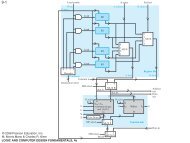
Mapped Circuit - Final Result<br />
D<br />
Y 1<br />
C<br />
R<br />
Z<br />
X<br />
D<br />
Y 2<br />
Clock<br />
Reset<br />
C<br />
R<br />
<strong>Chapter</strong> 5 - Part 2 33<br />
<strong>Sequential</strong> Design: Example 3<br />
• Design a sequential modulo 3 accumulator for 2-<br />
bit operands<br />
• Definitions:<br />
• Modulo n adder - an adder that gives the result of the<br />
addition as the remainder of the sum divided by n<br />
• Example: 2 + 2 modulo 3 = remainder of 4/3 = 1<br />
• Accumulator - a circuit that “accumulates” the sum of<br />
its input operands over time - it adds each input<br />
operand to the stored sum, which is initially 0.<br />
• Stored sum: (Y 1 ,Y 0 ), Input: (X 1 ,X 0 ), Output:<br />
(Z 1 ,Z 0 )<br />
<strong>Chapter</strong> 5 - Part 2 34<br />
17
Example 3 (continued)<br />
• Complete the state diagram:<br />
00<br />
Reset A/00<br />
01<br />
C/10<br />
B/01<br />
<strong>Chapter</strong> 5 - Part 2 35<br />
Example 3 (continued)<br />
• Complete the state table<br />
X 1 X 0<br />
Y 1 Y 0<br />
A (00)<br />
B (01)<br />
- (11)<br />
C (10)<br />
00<br />
Y 1 (t+1),<br />
Y 0 (t+1)<br />
00<br />
X<br />
01<br />
Y 1 (t+1),<br />
Y 0 (t+1)<br />
X<br />
• State Assignment: (Y 1 ,Y 0 ) = (Z 1 ,Z 0 )<br />
• Codes are in gray code order to ease use of K-maps in the next step<br />
11<br />
Y 1 (t+1),<br />
Y 0 (t+1)<br />
X<br />
X<br />
X<br />
X<br />
10<br />
Y 1 (t+1),<br />
Y 0 (t+1)<br />
X<br />
Z 1 Z 0<br />
00<br />
01<br />
11<br />
10<br />
<strong>Chapter</strong> 5 - Part 2 36<br />
18
Example 3 (continued)<br />
Y 0<br />
Y 1<br />
• Find optimized flip-flop input equations for D flip-flops<br />
X X<br />
X<br />
X<br />
Y 0<br />
X X X X X<br />
Y 1<br />
X<br />
X<br />
X<br />
D 1 X 1<br />
D 0 X 1<br />
X<br />
X<br />
• D 1 =<br />
• D 0 =<br />
X 0<br />
X 0<br />
<strong>Chapter</strong> 5 - Part 2 37<br />
Circuit - Final Result with AND, OR, NOT<br />
X 1<br />
X 0<br />
Z 0<br />
D<br />
Y 1<br />
Z 1<br />
C<br />
R<br />
D<br />
Y 0<br />
Reset<br />
Clock<br />
C<br />
R<br />
<strong>Chapter</strong> 5 - Part 2 38<br />
19
Other Flip-Flop Types<br />
• J-K and T flip-flops<br />
• Behavior<br />
• Implementation<br />
• Basic descriptors for understanding and<br />
using different flip-flop types<br />
• Characteristic tables<br />
• Characteristic equations<br />
• Excitation tables<br />
• For actual use, see Reading Supplement - Design<br />
and Analysis Using J-K and T Flip-Flops<br />
<strong>Chapter</strong> 5 - Part 2 39<br />
J-K Flip-flop<br />
• Behavior<br />
• Same as S-R flip-flop with J analogous to S and K<br />
analogous to R<br />
• Except that J = K = 1 is allowed, and<br />
• For J = K = 1, the flip-flop changes to the opposite<br />
state<br />
• As a master-slave, has same “1s catching” behavior<br />
as S-R flip-flop<br />
• If the master changes to the wrong state, that state<br />
will be passed to the slave<br />
• E.g., if master falsely set by J = 1, K = 1 cannot reset it<br />
during the current clock cycle<br />
<strong>Chapter</strong> 5 - Part 2 40<br />
20
J-K Flip-flop (continued)<br />
• Implementation<br />
• To avoid 1s catching<br />
behavior, one solution<br />
used is to use an<br />
edge-triggered D as<br />
the core of the flip-flop<br />
• Symbol<br />
J<br />
K<br />
C<br />
J<br />
K<br />
D<br />
C<br />
<strong>Chapter</strong> 5 - Part 2 41<br />
T Flip-flop<br />
• Behavior<br />
• Has a single input T<br />
• For T = 0, no change to state<br />
• For T = 1, changes to opposite state<br />
• Same as a J-K flip-flop with J = K = T<br />
• As a master-slave, has same “1s catching”<br />
behavior as J-K flip-flop<br />
• Cannot be initialized to a known state using the<br />
T input<br />
• Reset (asynchronous or synchronous) essential<br />
<strong>Chapter</strong> 5 - Part 2 42<br />
21
T Flip-flop (continued)<br />
• Implementation<br />
• To avoid 1s catching<br />
behavior, one solution<br />
used is to use an<br />
edge-triggered D as<br />
the core of the flip-flop<br />
• Symbol<br />
T<br />
T<br />
D<br />
C<br />
C<br />
<strong>Chapter</strong> 5 - Part 2 43<br />
Basic Flip-Flop Descriptors<br />
• Used in analysis<br />
• Characteristic table - defines the next state of<br />
the flip-flop in terms of flip-flop inputs and<br />
current state<br />
• Characteristic equation - defines the next<br />
state of the flip-flop as a Boolean function of<br />
the flip-flop inputs and the current state<br />
• Used in design<br />
• Excitation table - defines the flip-flop input<br />
variable values as function of the current<br />
state and next state<br />
<strong>Chapter</strong> 5 - Part 2 44<br />
22
D Flip-Flop Descriptors<br />
• Characteristic Table<br />
D<br />
0<br />
1<br />
Q(t+<br />
1)<br />
0<br />
1<br />
Operation<br />
Reset<br />
Set<br />
• Characteristic Equation<br />
Q(t+1) = D<br />
• Excitation Table<br />
Q(t +1)<br />
0<br />
1<br />
D<br />
0<br />
1<br />
Operation<br />
Reset<br />
Set<br />
<strong>Chapter</strong> 5 - Part 2 45<br />
T Flip-Flop Descriptors<br />
• Characteristic Table<br />
T Q(t+<br />
1)<br />
0<br />
1<br />
Q(t)<br />
Q(t)<br />
Operation<br />
No change<br />
Complement<br />
• Characteristic Equation<br />
Q(t+1) = T ⊕ Q<br />
• Excitation Table<br />
Q(t+1)<br />
Q(t)<br />
Q(t)<br />
T<br />
0<br />
1<br />
Operation<br />
No change<br />
Complement<br />
<strong>Chapter</strong> 5 - Part 2 46<br />
23
S-R Flip-Flop Descriptors<br />
• Characteristic Table<br />
S<br />
0<br />
0<br />
1<br />
1<br />
R<br />
0<br />
1<br />
0<br />
1<br />
Q(t+1)<br />
Q(t)<br />
0<br />
1<br />
?<br />
Operation<br />
No change<br />
Reset<br />
Set<br />
Undefined<br />
• Characteristic Equation<br />
Q(t+1) = S + R Q, S . R = 0<br />
• Excitation Table<br />
Q(t)<br />
Q(t+1) S R<br />
Operation<br />
0<br />
0<br />
1<br />
0<br />
1<br />
0<br />
0<br />
1<br />
0<br />
X<br />
0<br />
1<br />
No change<br />
Set<br />
Reset<br />
1<br />
1<br />
X<br />
0<br />
No change<br />
<strong>Chapter</strong> 5 - Part 2 47<br />
J-K Flip-Flop Descriptors<br />
• Characteristic Table<br />
0<br />
0<br />
1<br />
1<br />
• Characteristic Equation<br />
Q(t+1) = J Q + K Q<br />
• Excitation Table<br />
J<br />
K<br />
0<br />
1<br />
0<br />
1<br />
Q(t)<br />
Q(t+1)<br />
Q(t)<br />
0<br />
1<br />
Q(t)<br />
Q(t+ 1) J K<br />
Operation<br />
No change<br />
Reset<br />
Set<br />
Complement<br />
Operation<br />
0<br />
0<br />
1<br />
1<br />
0<br />
1<br />
0<br />
1<br />
0<br />
1<br />
X<br />
X<br />
X<br />
X<br />
1<br />
0<br />
No change<br />
Set<br />
Reset<br />
No Change<br />
<strong>Chapter</strong> 5 - Part 2 48<br />
24
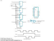
Flip-flop Behavior Example<br />
• Use the characteristic tables to find the output waveforms<br />
for the flip-flops shown:<br />
Clock<br />
D,T<br />
D<br />
Q D<br />
C<br />
T<br />
Q T<br />
C<br />
<strong>Chapter</strong> 5 - Part 2 49<br />
Flip-Flop Behavior Example<br />
(continued)<br />
• Use the characteristic tables to find the output waveforms<br />
for the flip-flops shown:<br />
Clock<br />
S,J<br />
R,K<br />
S<br />
C<br />
R<br />
Q SR<br />
?<br />
J<br />
C<br />
K<br />
Q JK<br />
<strong>Chapter</strong> 5 - Part 2 50<br />
25
Terms of Use<br />
• All (or portions) of this material © 2008 by Pearson<br />
Education, Inc.<br />
• Permission is given to incorporate this material or<br />
adaptations thereof into classroom presentations and<br />
handouts to instructors in courses adopting the latest<br />
edition of Logic and Computer Design Fundamentals as<br />
the course textbook.<br />
• These materials or adaptations thereof are not to be<br />
sold or otherwise offered for consideration.<br />
• This Terms of Use slide or page is to be included within<br />
the original materials or any adaptations thereof.<br />
<strong>Chapter</strong> 5 - Part 2 51<br />
26