Least-squares fitting of carrier phase distribution by using a rational ...
Least-squares fitting of carrier phase distribution by using a rational ...
Least-squares fitting of carrier phase distribution by using a rational ...

Create successful ePaper yourself
Turn your PDF publications into a flip-book with our unique Google optimized e-Paper software.
3588 OPTICS LETTERS / Vol. 31, No. 24 / December 15, 2006<br />
<strong>Least</strong>-<strong>squares</strong> <strong>fitting</strong> <strong>of</strong> <strong>carrier</strong> <strong>phase</strong> <strong>distribution</strong><br />
<strong>by</strong> <strong>using</strong> a <strong>rational</strong> function in fringe<br />
projection pr<strong>of</strong>ilometry<br />
Hongwei Guo, Mingyi Chen, and Peng Zheng<br />
Department <strong>of</strong> Precision Mechanical Engineering, Laboratory <strong>of</strong> Applied Optics and Metrology,<br />
Shanghai University, Shanghai 200072, China<br />
Received August 7, 2006; revised September 8, 2006; accepted September 22, 2006;<br />
posted October 2, 2006 (Doc. ID 73835); published November 22, 2006<br />
A least-<strong>squares</strong> <strong>fitting</strong> technique for the <strong>carrier</strong> <strong>phase</strong> component in fringe projection pr<strong>of</strong>ilometry is presented.<br />
The <strong>carrier</strong> <strong>phase</strong> <strong>distribution</strong> for an arbitrary measurement system can be perfectly described with<br />
a <strong>rational</strong> function, whose coefficients can be estimated <strong>by</strong> least-<strong>squares</strong> <strong>fitting</strong> to the measured reference<br />
<strong>phase</strong>s, so that the restrictions and limitations in the existing techniques are eliminated. © 2006 Optical<br />
Society <strong>of</strong> America<br />
OCIS codes: 120.2830, 120.5050, 150.6910.<br />
In fringe projection pr<strong>of</strong>ilometry, the depth maps <strong>of</strong><br />
object surfaces are calculated from the <strong>phase</strong> <strong>distribution</strong>s<br />
from which the <strong>carrier</strong> <strong>phase</strong>s have been removed.<br />
Therefore exactly determining the <strong>carrier</strong><br />
<strong>phase</strong> component is important for guaranteeing measurement<br />
accuracies. The difficulty is that the <strong>carrier</strong><br />
<strong>phase</strong> <strong>distribution</strong> generally contains nonlinearity in<br />
its pr<strong>of</strong>ile due to the restrictions <strong>of</strong> system schemes.<br />
In the conventional techniques, 1–4 this nonlinearity<br />
has been corrected on the bases <strong>of</strong> geometrical analyses<br />
<strong>of</strong> measurement systems. With these techniques,<br />
however, the system parameters must be known or<br />
adjusted carefully to satisfy some stringent conditions.<br />
The polynomial <strong>fitting</strong> methods 5–8 can overcome<br />
this problem, but with them the accuracies cannot<br />
be guaranteed even if high-degree polynomials<br />
are used because <strong>of</strong> their poor asymptotic properties;<br />
moreover, the error will increase when the data are<br />
extrapolated outside the reference plane. Reference 7<br />
suggests a <strong>rational</strong> function representation <strong>of</strong> the<br />
<strong>carrier</strong> <strong>phase</strong>s, but it assumes the optical axis <strong>of</strong> the<br />
imaging lens to be perpendicular to the reference<br />
plane, which is not always valid in measurement<br />
practice. To the best <strong>of</strong> our knowledge, models that<br />
can exactly describe the <strong>carrier</strong> <strong>phase</strong>s for an arbitrary<br />
measurement system are still not available.<br />
In this Letter, we demonstrate that the <strong>carrier</strong><br />
<strong>phase</strong> <strong>distribution</strong> for an arbitrary system can be<br />
perfectly represented with a 2D <strong>rational</strong> function.<br />
Based on this fact, a least-<strong>squares</strong> <strong>fitting</strong> technique<br />
for the <strong>carrier</strong> <strong>phase</strong> component is proposed. Because<br />
it is a pixelwise operation to remove the <strong>carrier</strong> component<br />
from the object <strong>phase</strong>s, we shall represent the<br />
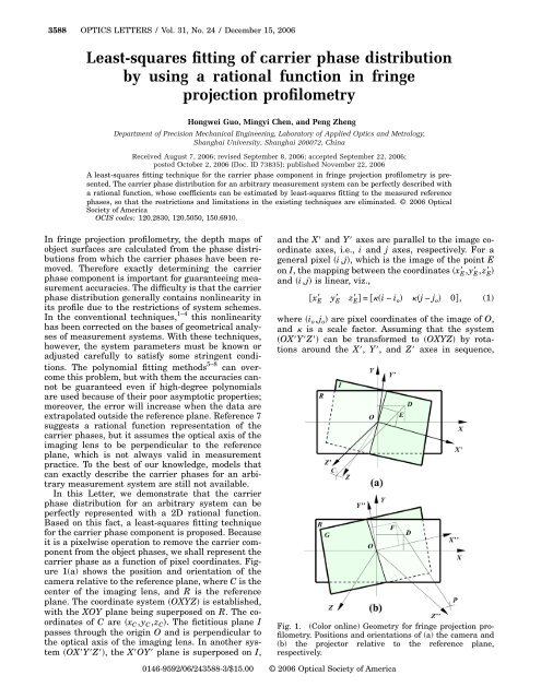
<strong>carrier</strong> <strong>phase</strong> as a function <strong>of</strong> pixel coordinates. Figure<br />
1(a) shows the position and orientation <strong>of</strong> the<br />
camera relative to the reference plane, where C is the<br />
center <strong>of</strong> the imaging lens, and R is the reference<br />
plane. The coordinate system OXYZ is established,<br />
with the XOY plane being superposed on R. The coordinates<br />
<strong>of</strong> C are x C ,y C ,z C . The fictitious plane I<br />
passes through the origin O and is perpendicular to<br />
the optical axis <strong>of</strong> the imaging lens. In another system<br />
OXYZ, the XOY plane is superposed on I,<br />
and the X and Y axes are parallel to the image coordinate<br />
axes, i.e., i and j axes, respectively. For a<br />
general pixel i,j, which is the image <strong>of</strong> the point E<br />
on I, the mapping between the coordinates x E ,y E ,z E <br />
and i,j is linear, viz.,<br />
x E y E z E = i − i o j − j o 0, 1<br />
where i o ,j o are pixel coordinates <strong>of</strong> the image <strong>of</strong> O,<br />
and is a scale factor. Assuming that the system<br />
OXYZ can be transformed to OXYZ <strong>by</strong> rotations<br />
around the X, Y, and Z axes in sequence,<br />
Fig. 1. (Color online) Geometry for fringe projection pr<strong>of</strong>ilometry.<br />
Positions and orientations <strong>of</strong> (a) the camera and<br />
(b) the projector relative to the reference plane,<br />
respectively.<br />
0146-9592/06/243588-3/$15.00 © 2006 Optical Society <strong>of</strong> America
December 15, 2006 / Vol. 31, No. 24 / OPTICS LETTERS 3589<br />
through the angles , , and (which are basic system<br />
parameters for determining the orientation <strong>of</strong><br />
the camera in 3D space), respectively, the coordinates<br />
<strong>of</strong> E in OXYZ can be calculated with<br />
x E<br />
y<br />
E <br />
cos sin 0<br />
1<br />
cos 0 − sin <br />
<br />
E = − sin cos 0 0 1 0<br />
z 0 0 sin 0 cos <br />
1 0 0 E <br />
0 cos sin y E <br />
2<br />
0 − sin cos x 0.<br />
The line CE crosses R at D. By utilizing the equation<br />
<strong>of</strong> CE, i.e., x−x C /x E −x C =y−y C /y E −y C =z<br />
−z C /z E −z C , the equation <strong>of</strong> R, i.e., z=0, and Eq. (2),<br />
the coordinates <strong>of</strong> D, x D ,y D ,z D , are calculated with<br />
x D<br />
y<br />
D x Cz E − x E z C /z E − z C <br />
<br />
D = y C z E − y E z C /z E − z C <br />
z 0<br />
1 x E + b 2 y E /1+a 1 x E + a 2 y E <br />
=b<br />
b 3 x E + b 4 y E /1+a 1 x E + a 2 y E , 3<br />
0<br />
where a 1 =−sin /z C , a 2 =sin cos /z C , b 1 =cos <br />
cos −x C sin /z C , b 2 =cos sin +sin sin cos <br />
+x C sin cos /z C , b 3 =−cos sin −y C sin /z C , and<br />
b 4 = cos cos − sin sin sin + y C sin cos /z C .<br />
Because D and E produce their images at the same<br />
pixel, the <strong>carrier</strong> <strong>phase</strong> at i,j equals the reference<br />
<strong>phase</strong> at D. That is,<br />
i,j = D .<br />
Figure 1(b) shows the relationship between the<br />
projector and R, where P is the center <strong>of</strong> the projector<br />
lens. The fictitious plane G passes through O and is<br />
perpendicular to the optical axis <strong>of</strong> the projector lens.<br />
Therefore the fringes projected on G are kept parallel<br />
to each other and are equally spaced with pitch p.<br />
The XOY plane <strong>of</strong> the system OXYZ is superposed<br />
on G, and the Y axis is parallel to the fringes.<br />
Assuming that OXYZ can be transformed to<br />
OXYZ <strong>by</strong> rotations around the X, Y, and Z axes<br />
in sequence, through the angles , , and , respectively,<br />
and that the coordinates <strong>of</strong> P in OXYZ are<br />
x P ,y P ,z P , the coordinates <strong>of</strong> D in OXYZ can be<br />
calculated with<br />
x D <br />
= 1 0 0<br />
<br />
cos 0 sin<br />
<br />
<br />
y D 0 cos − sin 0 1 0<br />
z D<br />
0 sin cos − sin 0 cos<br />
<br />
cos − sin 0<br />
1 x 0<br />
D<br />
sin cos 0 y D .<br />
5<br />
0 0<br />
4<br />
PD crosses G at F. By <strong>using</strong> the equation for PD, i.e.,<br />
x−x P / x D −x P =y−y P /y D −y P = z−z P /z D −z P ,<br />
the equation for G, i.e., z=0, and Eq. (5), the coordinates<br />
<strong>of</strong> F are obtained with<br />
x F P z D − x D z P /z D − z P <br />
y F y P z D − y D z P /z D − z P <br />
z F =x<br />
<br />
0<br />
= d 1x D + d 2 y D /1+c 1 x D + c 2 y D <br />
<br />
d 3 x D + d 4 y D /1+c 1 x D + c 2 y D , 6<br />
0<br />
where c 1 = cos sin cos − sin sin / z P , c 2<br />
=−cos sin sin +sin cos /z P , d 1 =cos cos +x P <br />
cos sin cos −sin sin /z P , d 2 =−cos sin −x P <br />
cos sin sin +sin cos /z P , d 3 =sin sin cos <br />
+cos sin +y P cos sin cos −sin sin /z P , and<br />
d 4 = −sin sin sin + cos cos − y P cos sin sin <br />
+sin cos /z P . Noting that DF is an equal-<strong>phase</strong><br />
line, we have<br />
D = F = O +2x F /p,<br />
7<br />
where O is the <strong>phase</strong> at O. Utilizing Eqs. (1), (3), (4),<br />
(6), and (7) yields<br />
i,j = r + si + tj/1+ui + vj,<br />
where u=a 1 + c 1 b 1 + c 2 b 3 /1 − a 1 + c 1 b 1 + c 2 b 3 i o<br />
− a 2 +c 1 b 2 + c 2 b 4 j o , v = a 2 + c 1 b 2 + c 2 b 4 /1<br />
−a 1 + c 1 b 1 + c 2 b 3 i o − a 2 + c 1 b 2 + c 2 b 4 j o , r = 0<br />
−2 d 1 b 1 + d 2 b 3 i o +d 2 b 4 +d 1 b 2 j o /p1−a 1 +c 1 b 1<br />
+c 2 b 3 i o −a 2 +c 1 b 2 +c 2 b 4 j o , s= 0 a 1 +c 1 b 1 +c 2 b 3 <br />
+2d 1 b 1 + d 2 b 3 /p/ 1 − a 1 + c 1 b 1 + c 2 b 3 i o − a 2<br />
+ c 1 b 2 + c 2 b 4 j o t = 0 a 2 + c 1 b 2 +c 2 b 4 +2 d 2 b 4<br />
+ d 1 b 2 /p/ 1− a 1 + c 1 b 1 +c 2 b 3 i o −a 2 +c 1 b 2 +c 2 b 4 <br />
j o . Differing from the existing methods, 5–8 Eq. (8)<br />
can exactly model the <strong>carrier</strong> <strong>phase</strong> map for an arbitrary<br />
system scheme.<br />
Derivation <strong>of</strong> Eq. (8) makes it possible in principle<br />
to determine the <strong>carrier</strong> <strong>phase</strong> <strong>distribution</strong> from the<br />
system parameters. However, the difficulty remains<br />
that these parameters are hard to know exactly. As<br />
an alternative approach, the coefficients <strong>of</strong> Eq. (8)<br />
can be estimated from the measured <strong>phase</strong> <strong>distribution</strong><br />
<strong>of</strong> a standard plane (i.e., reference plane). For<br />
simplifying the computation, we recast Eq. (8) in the<br />
following linear form,<br />
r + si + tj − ui,ji − vi,jj = i,j, 9<br />
8<br />
where the reference <strong>phase</strong> i,j has been measured.<br />
When i,j varies, a linear system based on Eq. (9) is<br />
established, from which r, s, t, u, and v can be solved.<br />
Using Eq. (9) involves a biased estimation, <strong>by</strong> which<br />
the expectations <strong>of</strong> the estimated coefficients in the<br />
presence <strong>of</strong> noise slightly deviate from their true values.<br />
Because the deviations are very small, the results<br />
are still satisfactory. If a higher accuracy is required,<br />
the nonlinear system based on Eq. (8) must<br />
be solved, and an iterative procedure has to be implemented.
3590 OPTICS LETTERS / Vol. 31, No. 24 / December 15, 2006<br />
In experiment, a standard plane is used as a reference,<br />
on which the checkerboard pattern is printed<br />
for implementing the lateral calibration simultaneously.<br />
In the scheme, the optical axes <strong>of</strong> both projector<br />
and camera incline to the reference plane, a<br />
case that cannot be well handled <strong>by</strong> the existing<br />
techniques. 1–8 The <strong>phase</strong>-shifting technique is used<br />
for <strong>phase</strong> recovery, and the sinusoid fringe patterns<br />
are projected with a DLP (digital light processing)<br />
projector, first on the reference plane and then on the<br />
tested object. The deformed patterns are captured <strong>by</strong><br />
a CCD camera. Figure 2(a) shows a pattern on the<br />
reference plane, from which the oblique perspective<br />
<strong>of</strong> the reference plane induced <strong>by</strong> the incline <strong>of</strong> the<br />
camera is easily observed. Figure 2(b) shows the recovered<br />
<strong>phase</strong>s. In the conventional techniques (see<br />
Ref. 9, for example) the <strong>carrier</strong> <strong>phase</strong>s are usually removed<br />
<strong>by</strong> subtracting the measured reference <strong>phase</strong>s<br />
from the object <strong>phase</strong>s. However, such a method is inoperable<br />
here, because the <strong>phase</strong> values are not<br />
available for the pixels inside the black boxes or outside<br />
the reference plane region. By <strong>fitting</strong> Fig. 2(b)<br />
with the <strong>rational</strong> function, the <strong>carrier</strong> <strong>phase</strong> <strong>distribution</strong><br />
can be reconstructed as shown in Fig. 2(c), where<br />
the lost data in Fig. 2(b) have been padded <strong>by</strong> interpolation<br />
or extrapolation. [The maximum difference<br />
between the <strong>phase</strong> maps reconstructed with Eqs. (8)<br />
and (9) is 0.009 rad, which is neglectable]. Figure 2(d)<br />
shows the residual <strong>of</strong> (b) subtracting (c), which consists<br />
mainly <strong>of</strong> the noises and the local deformations<br />
<strong>of</strong> the reference plane. With the proposed technique,<br />
such error factors are effectively eliminated.<br />
As indicated in Ref. 5, inaccurate <strong>carrier</strong> <strong>phase</strong>s<br />
will introduce additional bending (i.e., curvature errors)<br />
in the measurement results. This fact allows us<br />
to verify the validity <strong>of</strong> this technique <strong>by</strong> measuring a<br />
cylindrical object and then checking the resulting radius.<br />
For this purpose, a cookie jar is measured. In<br />
single-view measurements, we first recover the object<br />
<strong>phase</strong>s from the captured fringe patterns [one <strong>of</strong><br />
which is shown in Fig. 2(e)] and then subtract the<br />
<strong>carrier</strong> <strong>phase</strong>s in Fig. 2(c) from the object <strong>phase</strong>s. Finally,<br />
the 3D shape <strong>of</strong> each view is calculated <strong>by</strong> <strong>using</strong><br />
the mapping relationship between the <strong>phase</strong>s and<br />
depths. 9 By the registration <strong>of</strong> six views, 10 the 360°<br />
shape is obtained and shown in Fig. 2(f). Although<br />
additional errors may arise during the registration<br />
procedure, the final achieved accuracy depends<br />
mainly on single-view measurements. In Fig. 2(f), the<br />
least-<strong>squares</strong> radius <strong>of</strong> the cylinder is calculated as<br />
95.335 mm. As a comparison, the object is also measured<br />
<strong>by</strong> <strong>using</strong> a coordinate measuring machine, and<br />
the least-<strong>squares</strong> radius is obtained as 95.294 mm.<br />
From the results, the accuracy <strong>of</strong> this technique is<br />
evident.<br />
In conclusion, we have proposed a least-<strong>squares</strong> <strong>fitting</strong><br />
technique for determining the <strong>carrier</strong> <strong>phase</strong><br />
component. This technique <strong>of</strong>fers some important advantages<br />
over others. First, the model perfectly describes<br />
the <strong>carrier</strong> <strong>phase</strong> <strong>distribution</strong> for an arbitrary<br />
measurement system. Second, it allows for exactly<br />
determining the <strong>carrier</strong> <strong>phase</strong> map in the absence <strong>of</strong><br />
system parameters. Third, the influence <strong>of</strong> noise and<br />
local deformations <strong>of</strong> the reference plane on the measurement<br />
can be effectively restrained.<br />
This work was sponsored <strong>by</strong> the National Natural<br />
Science Foundation <strong>of</strong> China (60678036), and in part<br />
<strong>by</strong> Shanghai Leading Academic Discipline Project<br />
(Y0102). H. Guo’s e-mail address is hwguo@yeah.net.<br />
Fig. 2. (Color online) Experimental results. (a) Fringe pattern<br />
on the reference plane. (b) Phase map (in radians) reconstructed<br />
from (a). (c) <strong>Least</strong>-<strong>squares</strong> <strong>fitting</strong> result (in radians)<br />
<strong>of</strong> (b) <strong>using</strong> the <strong>rational</strong> function. (d) Residual (in<br />
radians) obtained <strong>by</strong> subtracting (c) from (b). (e) Deformed<br />
fringe pattern on the object. (f) Reconstructed 3D shape.<br />
References<br />
1. M. Takeda and K. Mutoh, Appl. Opt. 22, 3977 (1983).<br />
2. V. Srinivasan, H. C. Liu, and Maurice Halioua, Appl.<br />
Opt. 24, 185 (1985).<br />
3. M. Pirga and M. Kujawińska, Measurement 13, 191<br />
(1994).<br />
4. L. Salas, E. Luna, J. Salinas, V. García, and M. Servin,<br />
Opt. Eng. 42, 3307 (2003).<br />
5. L. Chen and C. Quan, Opt. Lett. 30, 2101 (2005).<br />
6. L. Chen and C. J. Tay, J. Opt. Soc. Am. A 23, 435<br />
(2006).<br />
7. Z. Wang and H. Bi, Opt. Lett. 31, 1972 (2006).<br />
8. L. Chen and C. Quan, Opt. Lett. 31, 1974 (2006).<br />
9. H. Guo, H. He, Y. Yu, and M. Chen, Opt. Eng. 44,<br />
033603 (2005).<br />
10. H. Guo and M. Chen, Opt. Eng. 42, 900 (2003).