DyBaNeM: Bayesian Framework for Episodic Memory Modelling

DyBaNeM: Bayesian Framework for Episodic Memory Modelling
Rudolf Kadlec (rudolf.kadlec@gmail.com)
Cyril Brom
Faculty of Mathematics and Physics
Charles University in Prague, Czech Republic
Abstract
Episodic Memory (EM) plays a central role in cognitive architectures
and artificial agents that need ability to remember
and recall the past. Most of the currently implemented EM
systems resemble logs of events stored in a database with indexes.
However, these systems usually lack abilities of human
memory like hierarchical organization of episodes, reconstructive
memory retrieval and encoding of episodes with respect
to previously learnt repeated schemata. Here, we present a
new general framework for EM modelling, DyBaNeM, that
has these abilities. From psychological point of view, it builds
on the Fuzzy-Trace Theory (FTT). On computational side, it
uses formalism of Dynamic Bayesian Networks (DBNs). We
describe abstract encoding, storage and retrieval algorithms,
two models we implemented within DyBaNeM, and evaluation
of the models’ performance using a dataset resembling a
log of human activity.
Keywords: Episodic Memory; Fuzzy Trace Theory; Dynamic
Bayesian Networks.
Introduction
EM (Tulving, 1983) is an umbrella term for memory systems
operating with personal history of an entity (as opposed to
semantic facts or procedural rules). Most EM systems implemented
to date capitalize on symbolic representations resembling
indexed logs of events. These data structures make it
hard to implement some of the most remarkable features of
human EM, such as hierarchical organization and reconstructive
retrieval.
The goal of this paper is to present a new framework for
EM modelling, DyBaNeM, in which these two features are
naturally emerging properties. We also present two models
implemented within this framework. The framework is inspired
by the FTT (Gallo, 2006). FTT hypothesizes two parallel
mechanisms that encode incoming information: verbatim
and gist. While verbatim encodes the surface-form of the
information in detail, gist encodes the meaning in a coarsegrained
way (Gallo, 2006), capitalizing on previously learnt
schemata (Bartlett, 1932) of episodes and parts of episodes.
There is also further evidence that people tend to perceive
episodes in a hierarchical fashion (Zacks & Tversky, 2001).
Models built within the DyBaNeM framework works as
follows. First the schemata of episodes are learned from annotated
examples modeling procedural learning during childhood.
Once learnt, the schemata remain fixed, becoming an
underlying structure for encoding, storage and episodic retrieval,
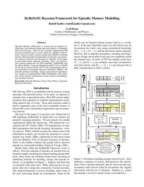
as exemplified on Figure 1. Suppose that Bob tries
to remember what Alice does. While observing her, he segments
what she is doing into a hierarchy of nested episodes.
This deduced hierarchy is used in encoding, where some of
the most interesting details are remembered. Some of the
details may be forgotten during storage (such as o 3 on Figure
1). In the end, when Bob wants to re-tell what he saw, he
reconstructs the whole story using remembered knowledge
(E2∼T 0 = c0 2∼T ;O 1 = o 1 ) and the previously learnt schemata.
However, due to imperfect perception, encoding and forgetting
in storage, the recalled events may not completely match
the original story. In terms of FTT the initially stored facts
O 1 = o 1 and O 3 = o 3 are verbatim, since they correspond to
real observations, and E2∼T 0 = c0 2∼T
is a gist because this is
Bob’s interpretation of Alice’s actions.
Alice
Bob
Bob’s perception
Bob’s storage Bob’s encoding
Bob’s retrieval
Deduced episodes
Gist
Verbatim
ρ 0
ρ 1
ρ 2
ρ 3
ρ T
a 1 0~T
b 0 0~1
c 0 2~T
o 0
o 1
o 2
o 3
o T
a 1 0~T
b 0 0~1 c 0 2~T
o 0 o 1
o 2 o 3
o T
E 0 2~T = c0 2~T
O 1
= o 1
O 3
= o 3
O 3 = o 3 forgotten
a 1 0~T
b 0 0~1
c 0 2~T
o 0
o 1
o 2
o 3
o T
Hi Alice, I remember
you doing o 1
so you
probably were doing
b 0 0~1
at that time.
Episodic
schemata
t
t
t
t
Stored
Observed
Reconstructed Reality
Figure 1: Perception-encoding-storage-retrieval cycle. Alice
performs a sequence of actions, Bob perceives this and deduces
Alice’s episodic hierarchy, then he stores encoded representation
until retrieval when he reconstructs the original
observation with the use of schemata. Notation x k i∼ j means
that episode x on level k started at time i and ended at j.

The presented framework uses Bayesian formalism. It implements
both the perception (where Bob segments Alice’s
behavior) and episode reconstruction in retrieval with the
same class of probabilistic models — DBN (Koller & Friedman,
2009). The underlying DBN is also heavily used in encoding.
In every step, different probabilistic queries are performed
over this model. Details of the model that had to be
omitted here due to space constraints are provided in (Kadlec
& Brom, 2013b). While the DBN formalism is widely used,
what is new here is exploration of its application on EM modelling.
FTT was previously implemented in a setting of static
scenes (Hemmer & Steyvers, 2009). Our work extends this
general approach also to sequences of events.
In the next section we discuss assumption of hierarchical
decomposition of behavior. Then we introduce our Dy-
BaNeM framework for EM modelling. In the end we evaluate
it using a corpora of hierarchically organized activities
and illustrate reconstructive recall in the model.
Hierarchical Activity Representation and
Probabilistic Models
One of the core assumptions of our framework is that flow of
events can be represented in a hierarchy of so called episodes.
This seem to be true both for humans (Zacks & Tversky,
2001) and for many computer controlled agents. Many formalisms
popular for programming agents in both academia
and industry use some kind of hierarchy, such as hierarchical
finite state machines or behavior trees.
At the same time, there is a body of literature on
using DBNs for activity recognition that also uses the
episode/activity hierarchy, e.g. (Bui, 2003; Blaylock & Allen,
2006). In activity recognition, DBNs-based models can be
used for deducing abstract episodes, that is, for computing
posterior probability of episodes conditioned on observations.
In EM modelling, we need also the inverse way; asking “what
if” queries: what is a retrieved memory of a situation given
the agent remembers two particular facts? Luckily, the DBNs
are flexible enough to allow for this “reverse” path.
DyBaNeM: Probabilistic EM Framework
In this section we introduce our EM framework. We start
with auxiliary definitions needed for description of the model.
Then we show how DBNs can be used for activity/episode
recognition and how the episodic schemata are represented
by two particular network architectures. Finally, we present
the algorithms of encoding, storage and retrieval.
Notation. Uppercase letters will denote random variables
(e.g. X,Y,O) whereas lowercase letters denote their values
(e.g. x,y,o). Probability mass function (PMF) of random variable
X will be denoted by P(X). When X is discrete, P(X)
will be also used to refer to a table specifying the PMF. Domain
of X will be denoted as D(X). Notation X i: j will be
a shorthand for sequence of variables X i ,X i+1 ...X j , analogically
x i: j will be a sequence of values of those variables. The
subscript will usually denote time. M will be a probabilistic
model and V is a set of all random variables in the model.
Formalizing the episodic representation, world state, and
inputs/outputs. In this section we formalize what representation
of episodes and world state is assumed by the Dy-
BaNeM framework.
Definition 1 Episode is a sequence (possibly of length 1)
of observations or more fine-grained episodes (sub-episodes)
that has a clear beginning and an end.
Note that episodes may be hierarchically organized.
Definition 2 Episodic schema is a general pattern specifying
how instances of episodes of the same class look like.
For instance, an episodic schema (cf. the notion of script or
memory organization packet (Schank, 1999)) might require
every episode derivable from this schema to start by event a,
then going either to event b or c and ending by d.
Definition 3 Episodic trace εt
0:n is a tuple 〈et 0 ,et 1 ...et n 〉 representing
a hierarchy of episodes at time t; et 0 is the currently
active lowest level episode, et 1 is its direct parent episode and
et n is the root episode in the hierarchy of depth n.
Example of an episodic trace can be ε 0:n
0
=
〈WALK,COMMUT E〉 and ε 0:n
1
= 〈GO BY BUS,
COMMUT E〉. The notation of episodic trace reflects the fact
that an agent’s behavior has often hierarchical nature.
Our model uses probabilistic representation, hence even if
there is only one objectively valid episodic trace for every
agent at each time step, input of the EM model will be a probability
distribution. Let Et i denotes a random variable representing
a belief about an episode on level i at time t. While
the true value of Et i is, say, et, i the PMF enables us to cope
with possible uncertainty in perception and memory recall.
Definition 4 Probabilistic episodic trace Et
0:n is a tuple of
random variables 〈Et 0 ,Et 1 ...Et n 〉 representing an agent’s belief
about what happened at time t. Analogically E0:t 0:n denotes
probabilistic episodic trace over multiple time steps.
The following data structure represents an agent’s true perception
of the environment state.
Definition 5 Let ρ t denotes observable environmental properties
at time t.
For instance, ρ can hold atomic actions executed by an
observed agent (and possibly other things too), e.g. ρ 0 =
STAND ST ILL, ρ 1 = GET TO BUS.
Analogically to Et 0:n and εt
0:n , O t is a random variable representing
belief about observation ρ t .
Fig. 2 shows how these definitions translate to an example
DBN structure. In this paper, we describe implementation of
two DBN-based models and the figure depicts both of them.
Surprise. In encoding, the framework works with quantity
measuring difference between the expected real state of a random
variable and its expected state given the remembered
facts. We call this quantity surprise. In Bayesian framework

E 0:n t:t+1
(n+1) th level
of episodes
2 nd level of
episodes
1 st level of
episodes
Observations
E 0:n t
O t:t+1
E n t
E 1 t
E 0 t
O t
H n t
H 1 t
H 0 t
F n t
F 1 t
F 0 t
E n t+1
E 1 t+1
E 0 t+1
O t+1
H n t+1
H 1 t+1
H 0 t+1
F n t+1
F 1 t+1
F 0 t+1
Figure 2: An example of a DBN’s structure together with
our notation. Solid lines show network architecture of
CHMM (Blaylock & Allen, 2006) model, whereas when the
dotted drawing is added we obtain network of AHMEM (Bui,
2003) model.
surprise can be defined as “difference” between prior and posterior
probability distributions. We adopt approach of (Itti &
Baldi, 2009) who propose to use Kullback-Leibler (KL) divergence
(Kullback, 1959) to measure surprise.
Definition 6 KL divergence (Kullback, 1959) of two PMFs
P(X) and P(Y ), where D(X) = D(Y ) is defined as:
KL(P(X) → P(Y )) =
∑
x∈D(X)
P(X = x)
P(X = x)ln
P(Y = x)
We use notation with → to stress directionality of KL divergence;
note that it is not symmetrical. We will use KL
divergence as a core tool of our framework. Another option
might be e.g. the Kolmogorov-Smirnov test.
Learning schemata
Episodic schemata are represented by parameters ˆθ of a DBN.
Expressiveness of schemata depends on the structure of a
model at hand. We will suppose that the DBN’s topology is
fixed. Thus learning schemata will reduce to well known parameter
learning methods. DBN with unobserved nodes has
to be learnt by Expectation-Maximization algorithm (EM algorithm),
topologies without unobserved nodes are learnt by
counting the sufficient statistics (Koller & Friedman, 2009).
In our case examples of episodes that we want to use
for schemata learning will be denoted by D = {d 1 ,d 2 ...d n }
where each d i can be one day of an agent’s live, or any other
appropriate time window. d i itself is a sequence of time
equidistant examples c t , that is, d i = {c i 0 ,ci 1 ...ci t i
}. Each ct i is
a tuple 〈εt
0:n ,ρ t 〉, it contains an episodic trace and observable
state of the environment.
DBN Architectures
For computing probabilities, our framework makes it possible
to use any DBN architecture where some nodes represent observations
and some probabilistic episodic trace. In this paper
we use two architectures, simple CHMM (Blaylock & Allen,
2006) and more complex AHMEM (Bui, 2003).
As we said the schemata are represented by parameter ˆθ,
that is, by all conditional probability mass functions (CPMFs)
of the DBN’s nodes. Expressiveness of the schemata depends
on the structure of DBN. In CHMM episodic schemata encode
probability of an episode given previous episode on the
same level in the hierarchy and also given its parent episode
(P(Et i |Et−1 i ,Ei+1 t )). This is one of possible hierarchical extensions
of a well known Hidden Markov Model (HMM).
CHMM is learnt by counting the sufficient statistic.
AHMEM is an augmentation of CHMM that extends each
episodic schema with a limited internal state (memory) represented
by a probabilistic finite state machine (PFSM) with
terminal states. This automaton is represented by random
variables Ft
i and Ht i in Fig. 2. This adds even more richness
to the represented schemata. Ht
i represents transition
between states of the PFSM (|D(Ht i )| is the number of the
PFSM’s states). Ft
i is a variable indicating that some states
of the PFSM are terminal, thus the episode has finished
(D(Ft i ) = {terminal,nonterminal}). Advatages of this model
are described in (Bui, 2003). Downside of the expressive
AHMEM models is that they are computationally more expensive
than CHMM. Since AHMEM contains unobservable
variables Ht i , it has to be learnt by EM algorithm.
Encoding
The encoding algorithm computes a list of mems on the basis
of the agent’s perception, Per 0:T , of the situation to be remembered.
Per 0:T is a set of PMFs such that Per 0:T = { f X :
X ∈ Observable}, where f X is PMF for each variable X of
interest. Now we have to distinguish what scenario we are
going to use:
1. Observable = O 0:T — Bob is going to encode Alice’s activity
whose ε Alice is hidden to Bob, nevertheless Bob perceives
Alice’s atomic actions that are contained in ρ Alice .
This is the use-case described in Figure 1. We introduce an
observation uncertainty by defining f Ot ≡ smoothed 1 ρ t ;
P(E 0:n
0:T
) will be deduced during the encoding algorithm.
2. Observable = E 0:n
0:T ∪ O 0:T — Bob is going to encode his
own activity, in this case the episodic trace ε Bob is available
since Bob knows what he wanted to do. Values of f Ot are
computed as above and f E i t
≡ smoothed e i t.
Algorithm 1 is a skeleton of the encoding procedure. The
input of the algorithm is Per 0:T , where the time window 0 : T
is arbitrary. In our work we use time window of one day. The
output is a list of mems encoding this interval.
1 For details of smoothing see (Kadlec & Brom, 2013b)

Algorithm 1 General schema of encoding algorithm
Require: Per 0:T — PMFs representing the agent’s perception
of the situation (i.e. smoothed observations)
Require: M — probabilistic model representing learned
schemata
1: procedure ENCODING(Per 0:T ,M )
2: mems ← empty ⊲ List of mems is empty
3: while EncodingIsNotGoodEnough do
4: X ← GetMem(M ,Per 0:T ,mems)
5: x max ← MLO PM (X|mems)
6: mems.add(X = x max )
7: end while
8: return mems
9: end procedure
The algorithm runs in a loop that terminates once the
EncodingIsNotGoodEnough function is false. There are
more possible stop criteria. We use |mems| < K because this
models limited memory for each day. Other possibilities are
described in (Kadlec & Brom, 2013b).
In each cycle, the GetMem function returns the variable
Xt i that will be remembered. The MLO function (most likely
outcome) is defined as:
MLO PM (X|evidence) ≡ argmaxP(X = x|evidence) (1)
x∈D(X)
This means that we get the most probable value for X and
add this assignment to the list of mems. 2 In the end the procedure
returns the list of mems.
We have developed two variants of the GetMem function,
each has its justification. In the first case, the idea is to
look for a variable whose observed PMF and PMF in the
constructed memory differs the most. This variable has the
highest surprise and hence it should be useful to remember it.
This strategy will be called retrospective maximum surprise
(RMaxS). It is retrospective since it assumes that the agent
has all observations in a short term memory store and, e.g.,
at the end of the day, he retrospectively encodes the whole
experience. RMaxS strategy can be formalized as:
X ← argmaxKL(P M (Y |Per 0:T ) → P M (Y |mems)) (2)
Y ∈VOI
where P(Y |Per 0:T ) ≡ P(Y |X = f X : f X ∈ Per 0:T ), we condition
the probability on all observations. VOI ⊆ V is a
set of random variables of interest whose value can be remembered
by the model. There can be some variables in
the DBN that we do not want to remember since they are
hardly interpretable for human. In our implementation we
used VOI = E0:T 0:n ∪ O 0:T .
The alternative strategy called retrospective minimum
overall surprise (RMinOS) assumes a more sophisticated pro-
2 Maximum a posteriori (MAP) (Koller & Friedman, 2009) query
would be more appropriate, we use MLO for simplicity.
cess. RMinOS picks the variable–value pair whose knowledge
minimizes surprise from the original state of each Y ∈
VOI to its recalled state. The following equation captures this
idea:
X ← argmin
Y ∈VOI
∑
Z∈V
KL
(P M (Z|Per 0:T ) → P M (Z|Y = ȳ,mems)) (3)
where ȳ ≡ MLO PM (Y |mems). Ideally, one should
minimize KL divergence from P(E0:T 0:n,O
0:T |Per 0:T ) →
P(E0:T 0:n,O
0:T |Y = ȳ,mems); however, that would require computing
the whole joint probability. Thus, we use summation
of surprise in each variable instead.
Note that we remember only the most probable value, including
the time index, in the mems list instead of the whole
distribution. This helps to make mems clearly interpretable.
However full distributions can be used in the mems as well.
Storage and forgetting
During storage, the mems can undergo optional time decayed
forgetting. The following equation shows relation between
age t of the mem m, its initial strength S and its retention R
(e is Euler’s number) (Anderson, 1983): R(m) = e − t S . The
initial strength S of mem m can be derived from the value
of KL divergence in Eq. 2 or from the value of the sum in
Eq. 3, respectively. Once R(m) decreases under the threshold
β f orget , m will be deleted from the list of mems and will not
contribute to recall of the memory.
Retrieval
Retrieval is a simple process of combining the schemata with
mems. Algorithm 2 shows this.
Algorithm 2 Retrieval
Require: k — cue for obtaining the episode
1: procedure RETRIEVAL(k,M )
2: mems ← getMemsFor(k) ⊲ List of mems associated
with the cue
3: return {P M (Y |mems) : Y ∈ VOI}
4: end procedure
We simply obtain the list of mems for search cue k, which
can be, e.g., a time interval. Then we use assignments in the
mems list as an evidence for the probabilistic model. The
resulting PMFs for all variables of interest are returned as a
reconstructed memory for the cue k.
Implementation
As a “proof-of-concept” of the DyBaNeM framework, we implemented
two models, AHMEM and CHMM, and two encoding
strategies RMaxS and RMinOS. The model was implemented
in Java and is freely available for download 3 . For
3 Project’s homepage http://code.google.com/p/dybanem

elief propagation in DBNs, SMILE 4 reasoning engine for
graphical probabilistic models was used.
Evaluation
Aim. We tested how the number of stored mems affects recall
accuracy when a model is applied to a dataset resembling human
activity. Multiple architectures of the underlying probabilistic
models were used to create several model variants.
We used both CHMM and AHMEM with one or two levels
of episodes. The CHMM models will be denoted as CHMM 1
or CHMM 2 , respectively. In the AHMEM we also variated
the number of states (|D(H i )|) of the PFSM consisting part
of episodic schemata. AHMEMs l denotes a model with l levels
and s states of internal memory. We tested AHMEM2 1, 1 8
and 2 2 . AHMEM2 8 required more than 1.5 GB RAM that was
dedicated to test and hence it was not tested. For each probabilistic
model we tested both RMaxS and RMinOS encoding
strategies and encoded one, two and three mems in turn.
Dataset. We used Monroe plan corpus (Blaylock & Allen,
2005) which is similar to real human activity corpus. Monroe
corpus is an artificially generated corpus of hierarchical
activities created by a randomized hierarchical task network
(HTN) planner. The domain describes rescue operations
like cutting up a fallen tree to clear a road, transporting
wounded to a hospital, etc. The corpus contains up to 9 levels
of episodes’ hierarchy, we shortened these episodic traces
to contain only the atomic actions and one or two levels of
episodes (based on the DBN used). The corpus features 28
atomic actions and 43 episodes.
Method. For the purpose of the experiment we split the
stream of episodic traces into sequences of 10, each of which
can be viewed as one day of activities. The schemata were
learned on 152 days. We tested accuracy of recall of atomic
actions that happened in one of randomly picked 20 days (out
of 152 days). Inference over the DBN was performed by exact
clustering algorithm (Huang & Darwiche, 1996).
Results. Tab. 1 summarizes recall performances of the
models. We use a simple crude accuracy measure that measures
how many actions were correctly recalled at correct
time. Only the most probable action at each step was used.
Discussion. To understand how well the models perform
we can construct a simplistic baseline model. The baseline
model would use mems only for storing observations (remembering
only verbatim, no gist) and recall the most frequent
atomic action for the time steps where no mem was
stored. Therefore the schema in this model would be represented
only by the most frequent action in the corpus, which
is NAV IGAT E V EHICLE appearing in 40% of time steps.
Thus the baseline model would score (40 + |mems| × 10)%
accuracy on average since we encoded only sequences of
10 observations for each day, thus remembering one mem
would increase accuracy by 10%. All models performed
4 SMILE was developed by the Decision Systems Laboratory
of the University of Pittsburgh and is available at
http://genie.sis.pitt.edu/
RMaxS
RMinOS
mems
1 2 3 1 2 3
arch
AHMEM2 1 55% 75% 93% 57% 77% 92%
AHMEM8 1 67% 88% 97% 64% 90% 98%
AHMEM 2 2 57% 78% 93% 53% 75% 93%
CHMM 1 53% 70% 85% 56% 71% 86%
CHMM 2 57% 69% 85% 59% 72% 87%
Table 1: Results of the recall experiment for all tested models,
encoding strategies and the number of stored mems.
better than the baseline. As expected, on average, it holds
that more complex probabilistic models better capture the
episodic schemata and hence have a higher recall accuracy. In
our experiment, AHMEM8 1 , the model with the highest number
of parameters, dominates all the other architectures. On
the other hand there are only subtle differences in the encoding
strategies RMaxS and RMinOS. Since RMaxS requires
less computational time, it should be preferred at least on domains
similar to ours.
Example of recall. We now demonstrate how the number
of stored mems affects the recalled sequence. In an encoded
example day only direct observations (values of O t ) ended
stored in the mems, however this does not have to be true in
general. Fig. 3 shows probability distributions when considering
different number of mems for recall of activities from
the example day. The mems are sorted according to the order
in which they were created by the encoding algorithm.
Hence we can visualize how the forgetting would affect recall
since the third mem is the least significant one and it
will be forgotten as the first, whereas the first mem will be
forgotten as the last. After forgetting all the mems the model
would return NAV IGAT E V EHICLE for each time point giving
us 30% accuracy because this action appears three times
in this particular sequence. This would be the same accuracy
as the baseline’s. With one mem a remembered episodic
schema is activated and accuracy grows to 50% (10% more
than the baseline). The second mem further specifies the activated
schema and changes the most probable action not only
in t = 9, which is the mem itself, but also in t = 3,5,6 and
8, and accuracy rises to 100% (50% more than the baseline).
The third mem removes the last uncertainty at t = 4.
Conclusion
We presented DyBaNeM probabilistic framework for EM
modelling. Evaluation has shown that increasingly complex
DBN architectures provide better episodic schemata and that
RMaxS strategy is sufficient for good encoding. Our model
can be used in general purpose cognitive architectures as well
as in virtual agents where it can increase an agent’s believability
(Kadlec & Brom, 2013a). We can see the framework
as a tool for lossy compression of sequences of events, thus
long living agents can plausibly store more memories in the

Figure 3: Recall of observation probabilities for 10 time steps (one day) in AHMEM8 1 + RMaxS model with increasing number
of mems used to reconstruct the sequence. Level of gray indicates probability of each atomic action at that time step.
The darker the color is the more probable the action is. The first figure shows P(O t ) for each time step in the remembered
sequence when only schemata are used, this is what the model would answer after forgetting all mems; the second shows
P(O t |O 0 = CLEAN HAZARD), recall with one mem; the third P(O t |O 0 = CLEAN HAZARD,O 9 = CUT T REE) and the
fourth P(O t |O 0 = CLEAN HAZARD,O 9 = CUT T REE,O 4 = REMOV E WIRE). The mems are marked by circles, all the
other values are derived from the schema that is most probable given the recalled mems. Only the relevant actions are shown.
same space. However the used probabilistic model has to be
chosen carefully since computational complexity of inference
in DBNs is high. On the other hand there are efficient approximation
techniques that can speed up the computation.
Our future work include learning the models using real human
corpora, e.g. (Kadlec & Brom, 2011), and comparing the
models’ outputs with data from psychological experiments.
.
Acknowledgments
This research was partially supported by SVV project number
267 314 and by grant GACR P103/10/1287. We thank to
xkcd.org for drawings of Alice and Bob.
References
Anderson, J. (1983). A spreading activation theory of memory.
Journal of verbal learning and verbal behavior, 22,
261–295.
Bartlett, F. (1932). Remembering: A Study in Experimental
and Social Psychology. Cambridge, England: Cambridge
University Press.
Blaylock, N., & Allen, J. (2005). Generating Artificial
Corpora for Plan Recognition. In L. Ardissono, P. Brna,
& A. Mitrovic (Eds.), Proceedings of the 10th international
conference on user modeling (UM’05) (pp. 179–
188). Edinburgh: Springer. Corpus is available from
www.cs.rochester.edu/research/speech/monroe-plan/.
Blaylock, N., & Allen, J. (2006). Fast hierarchical goal
schema recognition. Proceedings of the National Conference
on Artificial Intelligence (AAAI 2006), 796–801.
Bui, H. (2003). A general model for online probabilistic plan
recognition. International Joint Conference on Artificial
Intelligence, 1309–1318.
Gallo, D. (2006). Associative illusions of memory: False
memory research in DRM and related tasks. Psychology
Press.
Hemmer, P., & Steyvers, M. (2009). Integrating Episodic
and Semantic Information in Memory for Natural Scenes.
CogSci, 1557–1562.
Huang, C., & Darwiche, A. (1996). Inference in belief networks:
A procedural guide. International journal of approximate
reasoning(15), 225–263.
Itti, L., & Baldi, P. (2009). Bayesian surprise attracts human
attention. Vision research, 49(10), 1295–1306.
Kadlec, R., & Brom, C. (2011). Towards an automatic diary
: an activity recognition from data collected by a mobile
phone. In IJCAI workshop on Space, Time and Ambient
Intelligence (pp. 56–61).
Kadlec, R., & Brom, C. (2013a). DyBaNeM :
Bayesian Episodic Memory Framework for Intelligent Virtual
Agents. Intelligent Virtual Agents 2013, in press.
Kadlec, R., & Brom, C. (2013b). Unifying episodic memory
models for artificial agents with activity recognition problem
and compression algorithms : review of recent work
and prospects (Tech. Rep.).
Koller, D., & Friedman, N. (2009). Probabilistic graphical
models: principles and techniques. The MIT Press.
Kullback, S. (1959). Statistics and information theory. J.
Wiley and Sons, New York.
Schank, R. C. (1999). Dynamic memory revisited. Cambridge
University Press.
Tulving, E. (1983). Elements Of Episodic Memory. Clarendon
Press Oxford.
Zacks, J. M., & Tversky, B. (2001). Event structure in perception
and conception. Psychological bulletin, 127(1), 3–21.