DyBaNeM: Bayesian Framework for Episodic Memory Modelling
DyBaNeM: Bayesian Framework for Episodic Memory Modelling
DyBaNeM: Bayesian Framework for Episodic Memory Modelling

You also want an ePaper? Increase the reach of your titles
YUMPU automatically turns print PDFs into web optimized ePapers that Google loves.
E 0:n t:t+1<br />
(n+1) th level<br />
of episodes<br />
2 nd level of<br />
episodes<br />
1 st level of<br />
episodes<br />
Observations<br />
E 0:n t<br />
O t:t+1<br />
E n t<br />
E 1 t<br />
E 0 t<br />
O t<br />
H n t<br />
H 1 t<br />
H 0 t<br />
F n t<br />
F 1 t<br />
F 0 t<br />
E n t+1<br />
E 1 t+1<br />
E 0 t+1<br />
O t+1<br />
H n t+1<br />
H 1 t+1<br />
H 0 t+1<br />
F n t+1<br />
F 1 t+1<br />
F 0 t+1<br />
Figure 2: An example of a DBN’s structure together with<br />
our notation. Solid lines show network architecture of<br />
CHMM (Blaylock & Allen, 2006) model, whereas when the<br />
dotted drawing is added we obtain network of AHMEM (Bui,<br />
2003) model.<br />
surprise can be defined as “difference” between prior and posterior<br />
probability distributions. We adopt approach of (Itti &<br />
Baldi, 2009) who propose to use Kullback-Leibler (KL) divergence<br />
(Kullback, 1959) to measure surprise.<br />
Definition 6 KL divergence (Kullback, 1959) of two PMFs<br />
P(X) and P(Y ), where D(X) = D(Y ) is defined as:<br />
KL(P(X) → P(Y )) =<br />
∑<br />
x∈D(X)<br />
P(X = x)<br />
P(X = x)ln<br />
P(Y = x)<br />
We use notation with → to stress directionality of KL divergence;<br />
note that it is not symmetrical. We will use KL<br />
divergence as a core tool of our framework. Another option<br />
might be e.g. the Kolmogorov-Smirnov test.<br />
Learning schemata<br />
<strong>Episodic</strong> schemata are represented by parameters ˆθ of a DBN.<br />
Expressiveness of schemata depends on the structure of a<br />
model at hand. We will suppose that the DBN’s topology is<br />
fixed. Thus learning schemata will reduce to well known parameter<br />
learning methods. DBN with unobserved nodes has<br />
to be learnt by Expectation-Maximization algorithm (EM algorithm),<br />
topologies without unobserved nodes are learnt by<br />
counting the sufficient statistics (Koller & Friedman, 2009).<br />
In our case examples of episodes that we want to use<br />
<strong>for</strong> schemata learning will be denoted by D = {d 1 ,d 2 ...d n }<br />
where each d i can be one day of an agent’s live, or any other<br />
appropriate time window. d i itself is a sequence of time<br />
equidistant examples c t , that is, d i = {c i 0 ,ci 1 ...ci t i<br />
}. Each ct i is<br />
a tuple 〈εt<br />
0:n ,ρ t 〉, it contains an episodic trace and observable<br />
state of the environment.<br />
DBN Architectures<br />
For computing probabilities, our framework makes it possible<br />
to use any DBN architecture where some nodes represent observations<br />
and some probabilistic episodic trace. In this paper<br />
we use two architectures, simple CHMM (Blaylock & Allen,<br />
2006) and more complex AHMEM (Bui, 2003).<br />
As we said the schemata are represented by parameter ˆθ,<br />
that is, by all conditional probability mass functions (CPMFs)<br />
of the DBN’s nodes. Expressiveness of the schemata depends<br />
on the structure of DBN. In CHMM episodic schemata encode<br />
probability of an episode given previous episode on the<br />
same level in the hierarchy and also given its parent episode<br />
(P(Et i |Et−1 i ,Ei+1 t )). This is one of possible hierarchical extensions<br />
of a well known Hidden Markov Model (HMM).<br />
CHMM is learnt by counting the sufficient statistic.<br />
AHMEM is an augmentation of CHMM that extends each<br />
episodic schema with a limited internal state (memory) represented<br />
by a probabilistic finite state machine (PFSM) with<br />
terminal states. This automaton is represented by random<br />
variables Ft<br />
i and Ht i in Fig. 2. This adds even more richness<br />
to the represented schemata. Ht<br />
i represents transition<br />
between states of the PFSM (|D(Ht i )| is the number of the<br />
PFSM’s states). Ft<br />
i is a variable indicating that some states<br />
of the PFSM are terminal, thus the episode has finished<br />
(D(Ft i ) = {terminal,nonterminal}). Advatages of this model<br />
are described in (Bui, 2003). Downside of the expressive<br />
AHMEM models is that they are computationally more expensive<br />
than CHMM. Since AHMEM contains unobservable<br />
variables Ht i , it has to be learnt by EM algorithm.<br />
Encoding<br />
The encoding algorithm computes a list of mems on the basis<br />
of the agent’s perception, Per 0:T , of the situation to be remembered.<br />
Per 0:T is a set of PMFs such that Per 0:T = { f X :<br />
X ∈ Observable}, where f X is PMF <strong>for</strong> each variable X of<br />
interest. Now we have to distinguish what scenario we are<br />
going to use:<br />
1. Observable = O 0:T — Bob is going to encode Alice’s activity<br />
whose ε Alice is hidden to Bob, nevertheless Bob perceives<br />
Alice’s atomic actions that are contained in ρ Alice .<br />
This is the use-case described in Figure 1. We introduce an<br />
observation uncertainty by defining f Ot ≡ smoothed 1 ρ t ;<br />
P(E 0:n<br />
0:T<br />
) will be deduced during the encoding algorithm.<br />
2. Observable = E 0:n<br />
0:T ∪ O 0:T — Bob is going to encode his<br />
own activity, in this case the episodic trace ε Bob is available<br />
since Bob knows what he wanted to do. Values of f Ot are<br />
computed as above and f E i t<br />
≡ smoothed e i t.<br />
Algorithm 1 is a skeleton of the encoding procedure. The<br />
input of the algorithm is Per 0:T , where the time window 0 : T<br />
is arbitrary. In our work we use time window of one day. The<br />
output is a list of mems encoding this interval.<br />
1 For details of smoothing see (Kadlec & Brom, 2013b)