Odour Threshold Investigation 2012 - Bay of Plenty Regional Council

A review of odour properties of H 2 

S - 

Odour Threshold Investigation 2012 

Bay of Plenty Regional Council 

Environmental Publication 2012/06 

June 2012 

5 Quay Street 

P O Box 364 

Whakatane 

NEW ZEALAND 

ISSN: 1175-9372 (Print) 

ISSN: 1179-9471 (Online) 

Working with our communities for a better environment 

E mahi ngatahi e pai ake ai te taiao

A review of odour 

properties of H 2 S - Odour 

Threshold Investigation 

2012 

Environmental Publication 2012/06 

ISSN: 1175-9372 (Print) 

ISSN: 1179-9471 (Online) 

5 June 2012 

Bay of Plenty Regional Council 

5 Quay Street 

PO Box 364 

Whakatane 3158 

NEW ZEALAND 

Prepared by Shane Iremonger 

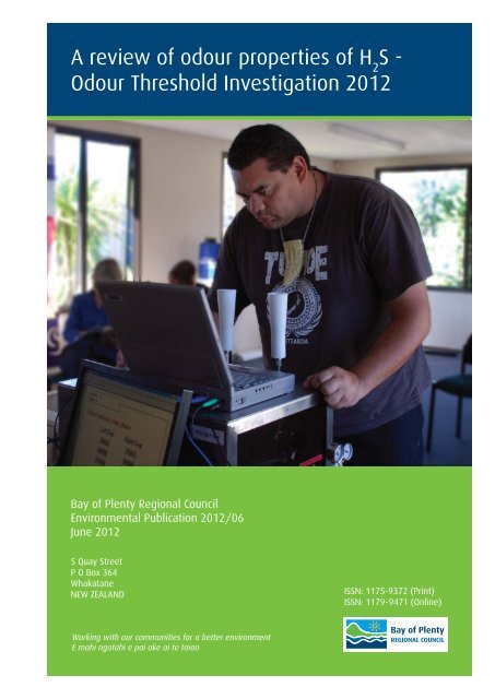
Cover Photo: 

A Rotorua panellist entering his choice following the presentation of 

sample gas at the olfactometer ports.

Acknowledgements 

Dr Bruce Graham for his peer review of this document. 

Dr Ray Littler for his statistical analysis guidance. 

The panellists - Paula, Natasha, Te Koringa, Roz, Greg, Nicola, Julie, Kenneth, Larraine, Kiri, 

Penny, Niki, Peter, Harpreet, Wayne, Graham, Craig, Lisa, Mike, Jo, Ian, Sherryn, Shelley, 

Vinoop, Kelly, Linda, Tipene, Rachel, Alan, John, Stephen, Nicholas, Des, Jacqui, Annabelle, 

Yves, Steven, Nassah, Jason, Joanne, Casey, Raewyn, Anya, Mel, Rose, Jo, Sue, Diane, 

Paul, Reece, Adrian, Jessica, Alastair, Shane, Scott, Janine, David, Wiki and Glenn. 

The support of the Bay of Plenty Regional Council Innovation Fund and its coordinators. 

Anya for her organisation and coordination of the panellist group. 

The Odour Unit Team. 

The document specialist skills of Rachael Musgrave, in the creation of this document. 

Environmental Publication 2012/06–A review of odour properties of H 2 S Odour Threshold Investigation 2012 

i

Executive Summary 

H 2 S is responsible for the characteristic ‘rotten eggs’ odour that most people would associate 

with geothermal areas. The odour can be detected at very low concentrations in air, and the 

level at which this first occurs is referred to as the odour threshold. This threshold varies from 

one person to the next, depending on individual sensitivities, age, state of health, and the 

conditions under which the odour is assessed. 

This project aims to establish an odour threshold for hydrogen sulphide (H 2 S) in air using 

local residents as the test subjects. This investigation looks at measuring and possibly 

refining the H 2 S odour threshold value by using dynamic dilution olfactometry (DDO) and a 

sample panel of 60 people. Half of the sample panel (30) consists of Rotorua residents, as 

they represent a group of people that are regularly exposed to elevated concentrations of 

ambient H 2 S. It is believed that this leads to a greater degree of tolerance of H 2 S odours, but 

it is not known whether this is due to a reduced sensitivity to the odour (i.e. a higher odour 

threshold). The other panellists (30) were from Whakatāne and Tauranga, where there is no 

exposure to geothermal sources of H 2 S. 

The primary questions for this investigation were – (i) what was the H 2 S detection threshold 

for a non-laboratory type screening panel and (ii) was there a difference in the results 

obtained for people living in an area with naturally high levels of H 2 S (Rotorua) and those 

living elsewhere? 

The threshold data calculations for this investigation have yielded a geometric mean 

concentration of 0.7 µg/m 3 when determined across the entire panel (n. = 59). The geometric 

means for the Rotorua and Whakatāne subgroups are 1.1 and 0.5 µg/m 3 respectively. These 

values are all well below the current New Zealand Ambient Air Quality guideline value of 

7 µg/m 3 . The geometric means are at the lower end of the summarised international 

threshold data. Discussion with olfactometry practitioners indicate that the results from this 

investigation are comparable with what they have recorded in laboratory type settings. 

The current NZAAQ guideline value of 7 µg/m 3 which was first documented nationally nearly 

20 years ago and discussed even earlier in a New Zealand context in the early 1980’s is still 

widely used as a starting point for odour assessments. For geothermal affected areas the 

common approach has been to use a value of 70 µg/m 3 , which was based on the historic 

New Zealand Health Department guideline. This value of 70 µg/m 3 meets the Good Practice 

Guide for Assessing Odour in New Zealand recommendation whereby for low sensitivity 

receiving environments the ambient concentrations can be in the order of 5-10 odour units 

(equivalent to 5 -10 times the odour threshold). 

However, using the threshold determined in this investigation the acceptable low sensitivity 

receiving environment values would only be in the order of 3.5 to 7 µg/m 3 , which as stated 

above is the value for non-geothermal (i.e. high sensitivity) areas. A guideline of 3.5 to 

7 µg/m 3 , is up to ten times lower than the value that is currently used for geothermal areas. 

However, based on community feedback and/or the lack of complaints about geothermal 

power plant emissions it appears these communities can tolerate 100 times the odour 

threshold determined in this study. 

This tolerance may well be due not to physiological changes in these people, but more so the 

acceptance of their location (which is often characterised by having a number of active 

geothermal surface features) and the economic and societal benefits associated with the use 

of the geothermal features/resource. 

Environmental Publication 2012/06–A review of odour properties of H 2 S Odour Threshold Investigation 2012 

i

In relation to the second question of this investigation the groups were spatially different, with 

one consisting of panellists from Whakatāne and Tauranga (non-geothermal areas) and one 

group from Rotorua, where the panellists are frequently exposed to concentrations well 

above the international literature odour thresholds. Other basic characteristics of the groups 

showed that they were generally similar in profiles when it came to the age and sex of the 

panellists. The residence time for the Rotorua panellists was also recorded. This was 

compared with threshold values for this group. The results showed no relationship with 

residence time and average measured threshold. 

Several types of analysis of the grouped data showed that there was a statistically significant 

difference between the geometric mean odour threshold results for the two groups (1.1 µg/m 3 

for Rotorua and 0.5 µg/m 3 for Whakatāne). The difference was small, but in the direction we 

would expect (Rotorua higher than non-geothermal locale). The results also showed that the 

human response to odour is highly variable. 

The difference between the two groups is interesting in a purely theoretical sense. However, 

when taking into account – (i) the wide range of thresholds that have been published to date, 

(ii) inaccuracies in the methodologies used in these investigations, and (iii) the end use 

application of thresholds as a comparison point for modelled outputs, the difference shown 

between the two groups would be regarded as insignificant and largely treated as being the 

same for both. The analysis showed that the vast majority of the panellists were able to 

detect H 2 S at the 7 µg/m 3 level. 

In setting a guideline value it would be dependent on the receiving environments location, as 

both groups appear “equal” when it comes to detecting. Variations in odour response would 

be dependent on what is commonplace in their local environment. Communities that live in 

close proximity to existing or proposed developments or natural settings where H 2 S 

emissions are present are equally adept at detecting the odour at low concentrations, when 

compared with the Whakatāne group, but more often than not would be accepting of the 

odour profile because of location. 

In regard to Council air quality policy, the findings of this investigation will be used in the 

upcoming Bay of Plenty Regional Air Plan review process. 

ii Environmental Publication 2012/06–A review of odour properties of H 2 S Odour Threshold Investigation 2012

Contents 

Acknowledgements 

i 

Part 1: Introduction 1 

Part 2: What is odour? 3 

2.1 The human response to odour 3 

2.2 Odour perception 3 

2.3 Human sensitivity to odours 4 

2.4 Cumulative effects, desensitisation/adaption and recovery 6 

2.5 Odour effects 7 

Part 3: H 2 S health effects 9 

Part 4: Sources of H 2 S in the Bay of Plenty 11 

4.1 Sources of H 2 S within the Bay of Plenty 11 

4.2 Ambient H 2 S levels within the Bay of Plenty 12 

Part 5: H 2 S threshold information 21 

5.1 International information 21 

5.2 National air quality criteria 23 

Part 6: Determination of an odour threshold value for hydrogen 

sulphide in the Bay of Plenty 27 

6.1 Outline 27 

6.2 Overview of the study methodology 27 

6.3 Specific aspects of the methodology relevant to this study 28 

6.4 Study locations 28 

Environmental Publication 2012/06–A review of odour properties of H 2 S odour threshold investigation 2012 

iii

6.5 Equipment 29 

6.6 Requirements of the panellist 29 

6.7 Calculation of odour concentration 30 

Part 7: Analysis of the results 33 

7.1 Testing room parameters 33 

7.2 Panel characteristics 35 

7.3 Result structure 36 

7.4 Incomplete rounds 37 

7.5 Hydrogen sulphide 39 

7.6 n-Butanol results 48 

Part 8: Discussion and conclusion 51 

8.1 Discussion 51 

8.2 Conclusion 53 

Appendix 1 – Olfactometer calibration sheet 57 

Appendix 2 – Calibration gas certification 59 

Appendix 3 – Dr Ray Littler analysis report 61 

iv Environmental Publication 2012/06–A review of odour properties of H 2 S odour threshold investigation 2012

Tables and Figures 

Table 3.1 Human health effects at various hydrogen sulphide concentrations. 9 

Table 4.1 Ambient recorded data summary for the Bay of Plenty. 19 

Table 7.1 Mean threshold values (µg/m 3 ) for all data and by location. 42 

Figure 2.1 Odorant receptors and the organisation of the olfactometry system. 4 

Figure 2.2 

Figure 2.3 

Figure 4.1 

The normal range concept showing a potential population distribution 

of olfactory sensitivities to odorants 5 . 5 

Relative slope of odour intensity for ammonia and hydrogen 

sulphide 5 . 6 

BOPRC complaints database output based on air complaint 

categories. 11 

Figure 4.2 Seasonal diurnal patterns recorded at Ti Street, Rotorua 15 

Figure 4.3 Ambient TRS data frequency from Awakaponga site. 16 

Figure 4.4 Ambient TRS data frequency from Edgecumbe site 49 . 17 

Figure 5.1 

Figure 6.1 

H 2 S threshold values from van Gemert (Note: data in red are 

additions which were sourced during the production of this report). 22 

Nalophan sample bag H 2 S concentrations (µg/m 3 ) measured with the 

Jerome during each day of testing, before and after rounds and as 

new bags were introduced to the testing. 31 

Figure 7.1 Room parameters for both locations during testing. 33 

Figure 7.2 Indoor H 2 S levels during testing in Rotorua. 34 

Figure 7.3 Effect of elevated ambient H 2 S level during testing. 35 

Figure 7.4 Graphical summaries of panellist characteristics. 36 

Figure 7.5 Ideal testing structure per panellist. 37 

Figure 7.6 Number of rounds recorded per panellist. 37 

Figure 7.7 

Example of incomplete rounds (Panellists 3 and 5) with individual 

thresholds still being determined upon “completion” of the round. 38 

Figure 7.8 Graphic of incomplete rounds and hence removed data points. 39 

Figure 7.8 Counts of threshold concentrations. 39 

Figure 7.9 Graphical summary of the “round” data. 40 

Environmental Publication 2012/06–A review of odour properties of H 2 S odour threshold investigation 2012 

v

Figure 7.10 Graphical summary of the “session mean” unconditioned data. 41 

Figure 7.11 Log 10 mean session data for the entire group and locations. 42 

Figure 7.12 

t-test results (with box plots) for a range of averaging levels and 

locations. 44 

Figure 7.13 H 2 S threshold range per session, all panellists. 44 

Figure 7.14 Trends per panellist per session (blue – Rotorua, red – Whakatāne). 45 

Figure 7.15 Trends per panellist by comparing first and last round results. 46 

Figure 7.16 Frequency plots - percentage of data points in relation to 7 µg/m 3 . 48 

Figure 7.16 Distribution patterns for n-Butanol. 50 

Figure 7.17 Scatterplot showing n-butanol and H 2 S relationship. 50 

Figure 8.1 Updated H 2 S threshold summary graph (adapted from Figure 5.1). 54 

Figure 1 (Data for this plot excludes Rotorua data with elevated ambient H 2 S). 62 

Figure 2 “affected” panellists have at least one result in the “suspect” period. 63 

Figure 3 Effects by panellist. 64 

Figure 6 Between session trends in log scale. 66 

Figure 7 Distribution of Whakatāne thresholds. 67 

vi Environmental Publication 2012/06–A review of odour properties of H 2 S odour threshold investigation 2012

Part 1: Introduction 

This project aims to establish an odour threshold for hydrogen sulphide (H 2 S) in air using 

local residents as the test subjects. As part of this project a summary of international and 

national threshold information and regional ambient monitoring data has been compiled in 

order to give the project threshold data some context. 

H 2 S is responsible for the characteristic ‘rotten eggs’ odour that most people would associate 

with geothermal areas. The odour can be detected at very low concentrations in air, and the 

level at which this first occurs is referred to as the odour threshold. This threshold varies from 

one person to the next, depending on individual sensitivities, age, state of health, and the 

conditions under which the odour is assessed. 

The odour threshold for H 2 S is often used in determining the potential for odour nuisance to 

arise as a result of certain discharges to air. This is a key factor in assessing the air 

emissions from geothermal developments, for which there appears to be a growing demand 

within the Bay of Plenty region. The threshold value will also be relevant to the assessments 

for other potential odorous sources, such as wastewater treatment plants, waste transfer 

stations and composting operations. 

The development of an odour threshold using local residents will help to ensure that the 

scientific and planning decisions around H 2 S discharges are soundly based and directly 

relevant to the region. 

Surprisingly, no work of this nature has been undertaken within New Zealand, even though in 

some areas H 2 S is a prominent part of the natural environment, whether it be from 

geothermal features in or around Taupo, Rotorua and Kawerau, or decomposing sea lettuce 

in the Tauranga Harbour upper tidal zones. 

National guidance documents have relied solely on international work when using the 

threshold values, and no locally-relevant thresholds have been formally determined. The 

need for local input is especially important for those areas that already experience a 

significant background H 2 S signature. 

There are a number of benefits of this investigation. Communities that live in close proximity 

to existing or proposed developments or natural settings where H 2 S emissions are present 

will benefit most from the increased certainty around decision making. There may also be 

benefits to developers, because the current approach, based on published data, appears to 

be quite conservative, in that it is assumed that people are more sensitive to H 2 S odour than 

suggested by actual experience. 

The published values for the odour threshold of H 2 S vary across a wide range of 

concentrations. These international and national values will be discussed in detail in Part 5. 

This report looks at measuring and possibly refining the H 2 S odour threshold value by using 

dynamic dilution olfactometry (DDO) and a sample panel of 60 people. 

Environmental Publication 2012/06–A review of odour properties of H 2 S odour threshold investigation 2012 1

The standardisation of DDO in Australasia and Europe has only occurred in the past ten to 

twenty years. The variability in the measurement method before standardisation means that 

earlier data are not necessarily comparable to the current measurements 1 . The 

recommended method for DDO in New Zealand (and Australia) is AS/NZS 4323.3:2001 2 , 

which was based on the European draft standard 3 . DDO and other techniques for odour 

measurement are described in detail in a central government technical report 4 , along with 

other less commonly used techniques, such as electronic instruments and chemical 

measurement of odorous compounds. 

This report follows the structure outlined below: 

Part 2 – Background information relating to how the human olfactometry system detects 

odour. 

Part 3 - A brief overview of H 2 S health effects. 

Part 4 - H 2 S odour sources and monitoring data for ambient H 2 S within the region. 

Part 5 - A summary of international and national odour threshold data for H 2 S. 

Part 6 - A description of the methodology used for this investigation. 

Part 7 - Statistical analysis of the measured data. 

Part 8 - A discussion of results and conclusions from the investigation. 

Data presented in this report will show different units. Quoted values will be as published, 

otherwise the unit convention will be to use μg/m 3 . Conversion between ppb and μg/m 3 can 

be undertaken using the following equation, H 2 S(μg/m 3 ) = 1.52 * H 2 S(ppb) at 0°C. 

1 

2 

3 

4 

Victorian EPA, 2002, Comparison of EPA approved odour measurement methods, Publication SR1. 

Australian/New Zealand Standard, 2001, Stationary Source Emissions. Part 3: Determination of Odour 

Concentration by Dynamic Olfactometry. 

European Committee for Standardisation, 2003, Air quality - Determination of odour concentration by 

dynamic olfactometry, EN 13725. 

Ministry for the Environment, 2002c, Review of Odour Management in New Zealand: Technical Report. 

Air quality technical report no. 24. Ministry for the Environment, Wellington, New Zealand. 

2 Environmental Publication 2012/06–A review of odour properties of H 2 S odour threshold investigation 2012

Part 2: What is odour? 

2.1 The human response to odour 

Odour is perceived by our brains in response to chemicals present in the air we 

breathe. Humans have the ability to detect odour even when chemicals are present 

in very low concentrations. 

Most odours are a mixture of many chemicals that interact to produce what we 

detect as an odour. Fresh air is usually perceived as being air that contains no 

chemicals or contaminants that could cause harm, or air that smells ‘clean’. 

However, fresh air may contain some odorous chemicals, but these will either be 

pleasant in character or at concentrations too low to be detected by humans. 

Different life experiences and natural variation in the population can result in 

different sensations and emotional responses by individuals to the same odorous 

compounds. Because the response to odour is synthesised in our brains, other 

senses such as sight and taste, and even our upbringing, can influence our 

perception of odour and whether we find it acceptable or objectionable and 

offensive. 

2.2 Odour perception 

A USEPA reference guide for odour thresholds states 5 that human odour perception 

has a few functional aspects of particular relevance: sensitivity and specificity. The 

close coupling of molecular odorant recognition events to neural signalling enables 

the nose to detect a few parts per trillion of some odorants 6 . The molecular nature of 

recognition permits the nose to distinguish between very similar molecules. 

The initial events of odour recognition (Figure 2.1) occur in a mucous layer covering 

the nasal epithelium, which overlays the convoluted cartilage in the back of the 

nasal cavity. Each of the millions of olfactory neurons in the middle layer of this 

epithelium extends a small ciliated dendritic knob to the surface epithelial layer and 

into the overlaying mucus. The binding of a single odorant molecule to a receptor on 

this dendritic tip may be adequate to trigger a neural signal to the brain. On each tip 

dozens of cilia increase the surface area available for recognition events ·and may 

stir the local mucus, aiding in the rapid detection of small concentrations of 

odorants. Individual receptors desensitize with use, temporarily losing their ability to 

transduce signals. 

The peripheral olfactory neurons project to the olfactory bulb from which signals are 

relayed to the olfactory cortex and more primitive brain structures such as the 

hippocampus and amygdala. This last structure affects whole brain-body emotive 

states. For further information on the olfactory system physiology, see Buck (2000) 7 . 

5 

6 

7 

USEPA, 1992, Reference Guide to Odour Thresholds for Hazardous Air Pollutants Listed in the Clean 

Air Act Amendments of 1990, Office of Research and Development, EPA/600/R-92/047. 

Reed RR, 1990, How does the nose know? Cell 60, 1–2. 

Buck, L., 2000, Smell and taste: the chemical senses. In Principles of Neural Science, E.R. Kandel, 

J. H. Schwartz, and T. M. Jessell, eds. (New York, McGraw-Hill), pp. 625-652. 


Figure 2.1 Odorant receptors and the organisation of the olfactometry system 8 . 

How an odour is perceived and its subsequent effects are not straightforward. The 

human perception of odour is governed by complex relationships, and its properties 

need to be considered when assessing potential odour effects. 

2.3 Human sensitivity to odours 

Our response to odours follows certain characteristic patterns common among most 

human sensory systems. For example, olfactory acuity in the population conforms to 

a normal distribution. Most people, assumed to be about 96% of the population, 

have a “normal” sense of smell as depicted in Figure 2.2. Two percent of the 

population are predictably hypersensitive and two percent insensitive. The 

insensitive range includes people who are anosmic (unable to smell) and hyposmic 

(partial smell loss). The sensitive range includes people who are hyperosmic (very 

sensitive) and people who are sensitised to a particular odour through repeated 

exposure. Another property of olfactory functioning includes adaptation to an odour, 

also known as olfactory fatigue. These terms describe a temporary desensitisation 

after being exposed to an odour 5 . 

8 

Courtesy of www.nobelprize.org/nobel_prizes/medicine/laureates/2004/odorant_high_eng.jpg. 

4 Environmental Publication 2012/06–A review of odour properties of H 2 S Odour Threshold Investigation 2012

Figure 2.2 

The normal range concept showing a potential population distribution 

of olfactory sensitivities to odorants 5 . 

Odour intensity refers to the perceived strength of the odour sensation. Intensity 

increases as a function of the concentration of the odorant chemical in the inhaled 

air. The relationship between perceived strength (intensity) and concentration can 

be expressed as a power function known as Stevens Law 3, 9 . In logarithmic 

coordinates Stevens Law becomes a linear function, the slope of which varies with 

the type of odorant over a range of about 0.2 to 0.7. In air pollution control this slope 

can be regarded as the “dose response” factor for odour effects. It also describes 

the degree of dilution necessary to decrease the intensity to ‘acceptable’ levels. A 

low slope value (such as H 2 S) would indicate an odour that requires a greater 

relative dilution for the odour to become non-detectable. The relative slope of H 2 S 

and ammonia are depicted schematically in Figure 2.3. The difference in slopes 

means that at high concentrations of both odorants the predominant odour will be 

that of ammonia, while at lower concentrations H 2 S will be detected. 

9 

Australian/New Zealand Standard, 2001, Stationary Source Emissions, Part 3: Determination of odour 

concentration by dynamic olfactometry, AS/NZS 4323.3:2001. 

Environmental Publication 2012/06–A review of odour properties of H 2 S Odour Threshold Investigation 2012 5

Figure 2.3 

Relative slope of odour intensity for ammonia and hydrogen 

sulphide 5 . 

As indicated by Stevens’ Law, the perception of the intensity of odour in relation to 

the odour concentration has a logarithmic relationship. The same relationship is 

known to occur for other human senses such as hearing and sensitivity to light. This 

means that if the concentration of an odour increases ten-fold, the perceived 

intensity will be approximately double (i.e. a two-fold increase). 

2.4 Cumulative effects, desensitisation/adaption and recovery 

In most situations a mixture of odorants, rather than just a single compound, will 

cause odour detection. One single compound may excite more than one type of 

olfactory receptor, while a different odorant is likely to excite a different subset of the 

350 types of human olfactory receptor cells. Studies have been undertaken on the 

perceived intensity of odour mixtures by mixing two odorants, both above the 

detection threshold. The typical finding was that the perceived intensity of a mixture 

is less than the arithmetic sum (hypo-addition) of the individual intensities. 

Interactions between mixtures of odorous compounds can also occur. An example is 

where one compound disguises or masks the presence of others. However, as the 

odour concentration reduces through dilution, the nature of the odour may change 

as different compounds dominate the effect; for example, mushroom-composting 

odour has been observed to have a distinctly different odour character at source 

than when diluted downwind. 

Continued exposure to an odour can result in people becoming desensitised so that 

they can no longer detect the odour even though the odorous chemical is constantly 

present in the air. This is sometimes known as ‘olfactory fatigue’. For example, 

people working in an environment with a persistent odour are often unaware of its 

presence and may not be aware that the odour is having an impact on the 

surrounding community. 


With continuing exposure to a certain odour concentration, the sensation gradually 

decreases, and may even disappear. Olfactory fatigue from continued exposure to 

an odour may affect a person’s sense of smell. This phenomenon is called 

adaptation 5, 10 . Adaptation begins to reduce perceived odour intensity and quality 

during the first inhalation. Adaptation may reduce both perceived odour intensity and 

perceived odour quality. Although adaptation takes some time to develop, recovery 

takes place more quickly. 

Ruijten et.al reports that while sensitivity to an odour may decrease after sniffing a 

sample, 80 to 90% recovery generally occurs within a minute with complete 

recovery in several minutes 3, 10 . 

Due to the special olfactory nature of H 2 S, during exposure, most subjects 

experienced an exponential decrease of intensity that dropped to a steady level 

within 2-5 minutes, and did not change appreciably up to 15 minutes later 11 . One of 

eight subjects indicated virtually complete loss of odour sensation and another 

substantial loss which is attributed to reversible paralysis of the olfactory nerve. The 

other six showed an approximately 50% decrease of perceived intensity, which 

corresponds to an apparent four-fold reduction in the H 2 S concentration. After 

breathing pure air, the sensitivity recovered almost completely in about four 

minutes 12 . 

2.5 Odour effects 

In New Zealand the nuisance effects of odour are commonly described by the term 

‘objectionable or offensive’. This concern with odour is regulated within the 

Resource Management Act (RMA) 13 . For some compounds, objectionable or 

offensive effects can occur at very low concentrations, usually far less than the 

concentrations associated with adverse health effects. However, other compounds 

only have objectionable or offensive effects at relatively high concentrations, at 

which point some of the contaminants in the odour may also be causing direct 

health effects such as skin, eye or nose irritation. Repeated or prolonged exposure 

to odour can lead to a high level of annoyance, and the receiver may become 

particularly sensitive to the presence of the odour. 

The health effects that have been reported as being associated with odour 

exposures include nausea, headaches, retching, difficulty breathing, frustration, 

annoyance, depression, stress, tearfulness, reduced appetite, and being woken in 

the night . There are also social effects such as reduced enjoyment of the outdoors 

and embarrassment in front of visitors. All of these contribute to a reduced quality of 

life for the individuals who are exposed. 

People can also develop physiological effects from odour even when their exposure 

is much lower than that normally associated with the reported health effects. This 

effect is sometimes termed ‘odour worry’ and is due to the perception that if there is 

a smell it must be doing physical harm. 

10 Shusterman, D, 1992, Critical Review: The Health Significance of Environmental Odour Pollution. 

Arch. Environ. Hlth 47: 76-88. 

11 Ekman, G., B. Berglund, U. Berglund, 1967, Perceived intensity of odour as a function of time 

adaptation. Scand. J. Psychol. 8: 177-186. 

12 Ruijten, M., van Doorn, R. & van Harreveld, A, 2009, Assessment of odour annoyance in chemical 

emergency management, National Institute of Public Health and the Environment, RIVM Report 

609200001/2009, The Netherlands. 

13 Resource Management Act (1991), Section 17 (3) (a) - “require a person to cease, or prohibit a person 

from commencing, anything that, in the opinion of the Environment Court or an enforcement officer, is 

or is likely to be noxious, dangerous, offensive, or objectionable to such an extent that it has or is likely 

to have an adverse effect on the environment.” 


Part 3: H 2 S health effects 

The primary focus of this report in on the odour threshold for H 2 S but for completeness and 

context a brief summary of health effect information is given below. This has been extracted 

from the World Health Organisation Concise International Chemical Assessment Document 

53 14 . 

Because hydrogen sulphide is a gas, inhalation is the major route of exposure to hydrogen 

sulphide. Most human data are derived from acute poisoning case reports, occupational 

exposures, and limited community studies. In confined spaces, human acute poisonings 

continue to occur. Single inhalation exposures to high concentrations of hydrogen sulphide 

cause health effects in many systems. Health effects that have been observed in humans 

following exposure to hydrogen sulphide include death and respiratory, ocular, neurological, 

cardiovascular, metabolic, and reproductive effects. 

Respiratory, neurological, and ocular effects are the most sensitive end-points in humans 

following inhalation exposures. There are no adequate data on carcinogenicity. 

A summary of human health effects resulting from exposure to H 2 S is presented in Table 3.1. 

Table 3.1 

Human health effects at various hydrogen sulphide concentrations. 

Exposure 

(mg/m 3 ) 

Effect/observation 

Reference 

0.011 Odour threshold. Amoore & Hautala, 1983 

2.8 Bronchial constriction in 

asthmatic individuals. 

Jappinen et al, 1990 

5.0 Increased eye complaints. Vanhoorne et al, 1995 

7 or 14 Increased blood lactate 

concentration, decreased 

skeletal muscle citrate 

synthase activity, decreased 

oxygen uptake. 

5-29 Eye irritation. IPCS, 1981 

28 Fatigue, loss of appetite, 

headache, irritability, poor 

memory, dizziness. 

Bhambhani & Singh, 1991; 

Bhambhani et al., 1996b, 

1997 

Ahlhorg, 1951 

>140 Olfactory paralysis. Hirsch & Zavala, 1999 

>560 Respiratory distress. Spolyar, 1951 

≥700 Death. Beauchamp et al, 1984 

14 WHO, 2003, Hydrogen Sulphide: Human Health Aspects. World Health Organisation, Geneva. Concise 

International Chemical Assessment Document (CICAD) No.53. 


Part 4: Sources of H 2 S in the Bay of Plenty 

4.1 Sources of H 2 S within the Bay of Plenty 

There is a wide range of possible odour sources in the Bay of Plenty region, some 

of which are associated with the numerous odour complaints received each year by 

the Bay of Plenty Regional Council (BOPRC) (see Figure 4.1). Total quantities of 

H 2 S emissions have not been determined for the Bay of Plenty, although some of 

the more major industrial sources have been documented. However, the spatial 

extent and variability of natural sources make this an unachievable task. 

Figure 4.1 

BOPRC complaints database output based on air complaint 

categories. 

Geothermal activity is one of the most common natural sources of H 2 S in the region 

(biogenic emissions 15 would be the most wide-spread) and occurs at a number of 

locations. Geothermal surface features extend from the northern boundaries of the 

Tauranga Harbour in the west, through to Manaohau springs located in Te Urewera 

National Park in the east. The northern extent of these features includes the 

offshore islands of Tuhua, Motuhora and Whakaari. Another significant natural 

source of H 2 S is decomposing sea lettuce in estuarine environments, particularly 

Tauranga Harbour. 

Anthropogenic sources within the Bay of Plenty include a number of industrial 

processes (which typically require air discharge permits 16 ) such as pulp mills, 

wastewater treatment plants, geothermal power generation, meat processing works, 

commercial composting operations and refuse transfer facilities. Domestic sources 

15 For example - coastal marine sediments. 

16 These permits may require ambient monitoring (Mighty River Power Ltd - 63298 and Carter Holt Harvey 

- 65725) or odour surveys (Tauranga City Wastewater Treatment plant - 62722 & 62723) to be 

undertaken depending on the scale of the operation. 


such as composting can provide very localised issues along with human flatulence 17 

(18ppm (~27mg/m 3 ) for humans on a normal diet). Internationally investigations into 

vehicular H 2 S sources have also been undertaken at several overseas locations , 

with an hourly maximum 18 of 54μg/m 3 and peaks 19 up to 150μg/m 3 being recorded. 

Rather that attempting to measure particular emission rates within the Bay of Plenty, 

ambient monitoring has been undertaken in various forms over the last 40 years at a 

number of locations within the region. This information is summarised below in order 

to provide an indication of the levels the population can be exposed to as they go 

about their daily activities and as context for the odour threshold studies. 

4.2 Ambient H 2 S levels within the Bay of Plenty 

Documentation of ambient levels varies in detail, ranging from a simple (but 

quantitative) categorisation of areas 20 to semi and fully quantitative H 2 S 

measurements. Odour surveys have also been undertaken at different times within 

the region 21, 22, 23 . These surveys are a consent requirement for some of the more 

substantial odour producing industrial activities. They do not require any H 2 S 

measurements as such, but are a qualitative way of determining odour influence 

and significance within a specific area of interest. 

4.2.1 Rotorua area 

Ambient monitoring of H 2 S has occurred in proximity to both natural and industrial 

sources. The Regional Council has monitored ambient H 2 S levels in Rotorua since 

the mid 1990’s 24 . Recorded levels for two of the longer periods of monitoring 

(at Ti Street and Arawa Street) show peak (one hour average) levels of up to about 

4000 µg/m 3 , and annual average concentrations of between 75 and 150 µg/m 3 

respectively. The data show clear diurnal patterns (Figure 4.2) which are most likely 

determined by meteorological factors such as wind speed and direction, 

atmospheric stability and rainfall. 

17 ATSDR, 2006, Agency for Toxic Substances and Disease Registry ToxGuide for Hydrogen Sulfide, 

CAS#7783-06-4, July 2006. 

18 Kourtidis, K., Kelesis, A., Petrakakis, M., 2008, Hydrogen sulphide in urban air, Atmospheric 

Environment, vol 42, 7476 - 7482. 

19 Deuchar, C. N., 2002, The Detection and Measurement of Hydrogen Sulphide, A thesis submitted 

to the University of Nottingham for the degree of Doctor of Philosophy in the School of Life and 

Environmental Sciences. 

20 Bates, M. N., Garrett, N., Shoemack, P., 2002, Investigation of health effects of hydrogen sulphide from 

a geothermal source, Arch. Environ. Health, 57(5), 405-411. 

21 Tauranga City Council, 2012, Tauranga Biannual Community Odour Survey 2012, A requirement of the 

Resource Consents for the Chapel Street and Te Maunga Wastewater Treatment Plant, September 

2012. 

22 Mighty River Power, 2009, Mighty River Power Kawerau Geothermal Power Station Odour Survey 

Report, prepared for Mighty River Power by Beca Infrastructure Limited. 

23 Carter Holt Harvey Tasman Limited, 2007, Carter Holt Harvey Tasman Kraft Pulp Mill Odour Survey 

Report 2007, Prepared for Carter Holt Harvey Tasman Limited by Beca AMEC Limited, March 2007. 

24 Iremonger S, 2004. NERM Air Monitoring Review. Environment BOP, Whakatane. Environmental 

Publication No. 2004/03. 


City wide measurements were also undertaken by Horwell 25 using a novel 

qualitative passive sampler approach. A method involving the reaction of H 2 S with 

the silver halide contained in treated photographic paper was developed and tested. 

Based on the analysis of the results Rotorua city was divided into three regions, an 

area of low concentrations in the west of the city, a corridor of high concentrations in 

the centre of the city, and an area of medium concentrations in the east of the city. 

During the project continuous gas detector measurements were also undertaken 

with a paper tape toxic gas detector 26 at three locations, Jervis Street located 

approximately 1 km northwest of the Arikikapakapa geothermal area, Ruihi Street, 

central city 1 km northwest of the racecourse and a lake front location. All 

deployments were for periods of several months. 

For Jervis Street the average concentration was ~5 ppb with occasional spikes 

reaching 90 ppb, with concentrations in the range of 20-30 ppb commonly being 

recorded during the night. The lake front site was monitored for a period between 

August 1997 and November 1997, and the 90 ppb instrument limit was exceeded 

about 40 times during the deployment. The average concentration from September 

to November was 1.3 ppb. The Ruihi Street deployment collected 15 days of record, 

4.2% of the time values were above the instrument maximum of 90 ppb. An average 

over the 15 days was 11 ppb. Approximately 50% of the time values were

Seigel et al 32 undertook measurement of H 2 S at 32 sites within Rotorua City. 

“Metronics Rotorod Colortec” asbestos pads treated with lead acetate were used to 

obtain hourly spot measurements over a 12 hour daily measurement window. 

Values ranged from

Figure 4.2 

Seasonal diurnal patterns recorded at Ti Street, Rotorua 

Source or near source measurements 

In Rotorua there have been a number of projects looking at levels of H 2 S. 

Finlayson 40 investigated soil gas levels which showed an isolated but significant 

concentration zone at Arikikapakapa and a north/south alignment of zones of higher 

concentration (20,000 – 200,000 ppm), that starts at the edge of Whakarewarewa, 

proceeds north with increasing concentrations and a greater area of significant gas 

emissions, terminating at Government Gardens. 

Indoor H 2 S measurements were undertaken by Durand & Scott 41 . The primary 

means of gas entry was directly from the ground through the floors, walls, and 

subsurface pipes. Indoor vents were located and found emitting up to approximately 

200 ppm H 2 S, concentrations high enough to present an acute respiratory hazard to 

persons close to the vent (e.g. children playing at floor level). These confined space 

levels are significantly higher than ambient levels. 

Smid et. al 42 reported on direct source measurements from 38 geothermal features 

including fumaroles, acid pools, alkaline springs, collapsed craters, mud pools, mud 

cones, and warm ground. H 2 S gas concentrations in parts per million (ppm) were 

recorded using a personal H 2 S monitor, the Dräger Pac 7000 43 , calibrated with a 

data logger interval set at 10 seconds. H 2 S gas readings were taken at the 

surface/entry of the feature, 0.5 meters above the surface/entry, and 1 m above the 

surface/entry. Overall, features emitted concentrations of H 2 S gas from 0 to 

100+ ppm at the feature entries. At a height of 0.5 m above feature surface/entry, 

H 2 S readings ranged from 0 to 57 ppm. At 1 m above feature surface/entry, the H 2 S 

measurements ranged from 0 to 20 ppm. 

40 Finlayson, J.B., 1992, A soil gas survey over Rotorua Geothermal Field, Rotorua, New Zealand, 

Geothermics, Vol. 21 No. 1/2, ISSN 0375-65058. 

41 Durand, M. & Scott, 2005, Geothermal ground gas emissions and indoor air pollution in Rotorua, 

New Zealand, Sci. Total Environ, 345, 69-80. 

42 Smid, E. R., Howe, T. M. & Lynne, B. Y.,2010, H 2 S Pilot Study, Rotorua, New Zealand, Institute of 

Earth Science and Engineering, New Zealand, Report 11-2010.1, April 2010. 

43 Electrochemical diffusion device. 


Rotorua District Council also undertakes regular monitoring of H 2 S levels within 

Rotorua. This monitoring typically has an indoor or enclosed space focus. The 

Council administers the Geothermal Safety Bylaw 44 and provides an advisory role, 

which includes testing for the presence of H 2 S gas to ensure as far as possible, the 

safety of public from geothermal activity. The levels monitored can be as high as 

several hundred ppm on occasions 45 . 

4.2.2 Kawerau area 

Carter Holt Harvey Pulp and Paper Limited at the Tasman Mill continuously monitor 

ambient TRS 46 at Edgecumbe 47 (and also historically at Awakaponga 48 ) (see 

Figures 4.3 and 4.4 respectively). This monitoring builds on earlier investigative 

monitoring undertaken during 1992 which looked at total sulphur levels 49 where a 

H 2 S guideline value of 7μg/m 3 was exceeded for 4.8 percent of the time over the 

seven month (mainly winter time) monitoring period. 68 

A key issue relating to the Rangitāiki Plains ambient monitoring is that the data 

records TRS. These measurements therefore include H 2 S emissions from the 

Norske Skog Turbo Alternator 3 electricity generator stack, a number of the Carter 

Holt Harvey pulp mill stacks, and the geothermal surface features located in the 

Kawerau township and the hills to the west. The percentage contribution made by 

H 2 S to the TRS readings is unknown, and may vary from hour to hour depending on 

both natural and industrial geothermal emissions. 

Figure 4.3 Ambient TRS data frequency from Awakaponga site 50 . 

44 Rotorua District Council, 2008, Geothermal Safety Bylaw, Doc No: IT-621891. 

45 Pers. Comms Peter Brownbridge, RDC Geothermal Inspector. 

46 Total Reduced Sulphur - includes hydrogen sulphide, mercaptans, dimethyl sulphide, dimethyl 

disulphide and other sulphur compounds. 

47 Resource Consent 60725 

48 Resource Consent 61435 

49 Bingham, A.G. et al, 1992, Ambient Air Quality Monitoring – Edgecumbe, 1992. Institute of 

Environmental Health & Forensic Sciences, NECAL Report S92/837C, 5 August 1992, 27p. 

50 Resource Consent 65720 Assessment of Environmental Effects, Chapter 4. 


Figure 4.4 Ambient TRS data frequency from Edgecumbe site 50 . 

Mighty River Power Ltd – Kawerau Geothermal Power Station has also undertaken 

limited ambient monitoring as required by their air discharge consent 51 at a location 

at the adjacent Tasman Mill, and at the three nearby townships of Kawerau, 

Edgecumbe and TeTeko. 

The results 52 show that short term (10-15 minute average) concentrations of H 2 S 

can reach 924 μg/m 3 at the Mill site, over 120 μg/m 3 at the Kawerau site 53 , up to 30 

μg/m 3 at the TeTeko site, and up to 70 μg/m 3 at the Edgecumbe site. The longer 

term concentrations, indicated by the annual averages, can reach 7.0 μg/m 3 at the 

Mill site, over 3.8 μg/m 3 at the Kawerau site, 0.3 μg/m 3 at the Te Teko site, and 0.9 

μg/m 3 at the Edgecumbe site. 

Under a consent change Mighty River Power Ltd are now required to undertake 

ambient H 2 S monitoring 54 for a period of not less than 24 months in relation to the 

operation of their geothermal plant near Kawerau township. The gas analyser 

monitoring equipment is currently being installed at monitoring sites at the north end 

of the Kawerau Township, Edgecumbe and Te Teko. 

4.2.3 Rotomā area 

Kingston Morrison 55 also reports on H 2 S monitoring carried out at Rotomā. On 

3 April 1995 the monitoring equipment was located at Rotomā School for several 

months. H 2 S levels were frequently above 7 μg/m 3 and up to approximately 22 

μg/m 3 were reported. These higher concentrations mostly occurred at night. 

51 Resource Consent 63298 Assessment of Environmental Effects, Air Quality documentation. 

52 Fisher, G.W., 2009, Ambient Monitoring Analysis, Assessment of Effects of the Discharges from the 

Proposed Kawerau Geothermal Power Station, prepared for Mighty River Power, 5 August 2009, 26p. 

53 Although probably high concentrations since the instrument has exceeded its scale. 

54 BOPRC Air discharge consent 63298. 

55 Kingston Morrison, 1995, Rotomā Geothermal Field Chemistry of Discharge Fluids from Well RM1 for 

Power NZ, Works Geothermal Report P164703. 


Kevern 56 undertook several surveys (20/8/93, 10/9/93 and 17/9/93) using a Jerome 

Model 621 sensor with a H 2 S detection range of 0-50 ppb. Measurement points 

were at irregular intervals along the State Highway from Kawerau to Rotorua. 

Results showed that the H 2 S level around Rotoehu/Rotoma were below 5 ppb. 

Kevern noted that samples taken at the Waitangi Soda Springs on 10 September 

were high (up to 45 ppb) compared to the values recorded on 17 September and 

attributed this to possibly a contamination of the measurement cell from high 

readings recorded in Rotorua earlier in the day. Elevated levels were found in the 

Kawerau, Tikitere and Rotorua areas (15->50 ppb). 

4.2.4 Tauranga Harbour 

Monitoring of ambient H 2 S associated with decomposing sea lettuce 57 has shown 

concentrations that are at adverse human health effect levels. Two sites in 

Tauranga Harbour, Ongare Point and Ngakautuakina Point, were selected for 

monitoring of H 2 S based on reported odour issues and health concerns raised by 

local residents. When the material was disturbed, both sites recorded values greater 

than ~288,000 μg/m 3 . Values recorded ~1 m above the surface ranged from 2.88 

mg/m 3 to 14.4 mg/m 3 . 

A summary of the ambient values from this section are shown in Table 4.1. For the 

purposes of comparison all H 2 S volume measurements have been converted to 

weight-based measurements (see Section 1). It should be noted that the results 

obtained by different measurement methods may not be directly comparable 

(sampling inlet position has been noted where known). No allowance has been 

made for the different measurement sampling and averaging times. 

The summary table shows that a wide range of concentrations can be experienced 

depending on location. Also at any given location there can be variations of several 

orders of magnitude in the values monitored, most likely due to variations in 

emissions and/or meteorological conditions. 

56 Kevern, R., 1993, BOPRC Internal memorandum, Ambient Hydrogen Sulphide Monitoring around 

Lake Rotoma, File Reference 1370 03 0077, 5p. 

57 BOPRC, 8 December 2009, Tauranga Harbour sea lettuce - hydrogen sulphide monitoring, Agenda 

Report to Regulation Monitoring & Operations Committee. 


Table 4.1 

Ambient recorded data summary for the Bay of Plenty. 

Ambient recorded data summary for the Bay of Plenty (µg/m 3 ). 

Data interval Data interval 

Location Peak Hourly Annual Location Peak Hourly Annual 

Tasman Mill, Kawerau 51 924 7 Rotorua central 1000 34 150 32 

Te Teko 51 30 0.3 Rotorua western 32

Part 5: H 2 S threshold information 

Odour threshold literature for a particular chemical can provide a wide range of threshold 

values and, as highlighted within this section, this is certainly the case for H 2 S. Often the 

disparity stems, in part, from inter-individual differences in sensitivities to odours, and in part, 

from methodological differences 58,59 . Warner 60 has also stated that the widely varying odour 

thresholds for H 2 S, some three orders of magnitude, are generally ascribed to olfactory 

desensitisation, which is a characteristic of the gas. 

The Good Practice Guide for Assessing and Managing Odour in New Zealand 61 states that 

published odour threshold data should be used with caution because many different methods 

have been used and there is a wide variation reported in the literature, often by four orders of 

magnitude. As an example, when using dilution dynamic olfactometry methods the odour 

threshold is usually taken as the value at which 50 percent of the panel are able to detect or 

recognise the odour, but some historical data are based on a range of different percentages. 

Most odour threshold reference data appear to have been developed before dilution dynamic 

olfactometry was standardised, so the data may not be directly applicable to assessments 

where odour guidelines have been developed based on the standard olfactometry 

techniques. 

Both detection and certainty, or recognition, odour thresholds for compounds are reported in 

the literature. The detection threshold is the lowest concentration of a compound that can 

just be detected by a certain percentage of the population, while the certainty or recognition 

threshold is the lowest concentration of a compound that can be recognised with certainty as 

having a characteristic odour quality. In general, recognition thresholds are approximately 

three to five times the detection threshold. When using odour threshold data it is important to 

be clear about which type of threshold is being reported. 

This section lists references for H 2 S threshold data. The majority of the information is from 

international publications, while the information from local sources relates mainly to the use 

of threshold data in establishing air quality guidelines. 

5.1 International information 

Van Gemert 62 provides a compilation of published odour threshold data for a wide 

range of chemical substances. The data for H 2 S is summarised in Figure 5.1, and 

covers studies from as far back as 1848. The data are given chronologically for 

each compound with the original data source identified, but no attempt is made by 

the author (van Gemert) to critically evaluate the data. Van Gemert’s publication is 

an update of similar previous compilations, such as Devos et al 63 . In addition to van 

Gemert’s data, data points (shown in red) have been added as a result of a 

literature search undertaken during the production of this report. 

58 van Harreveld, A.P., Heeres, P. & Harssema, H., 1999, A Review of 20 Years of Standardization of 

Odour Concentration Measurement by Dynamic Olfactometry in Europe, J. Air & Waste Manage. 

Assoc., 49:705-715. 

59 Ramsdale, S.L. and Baillie, C.P, 1996, Inter laboratory Test Program: Odour Detection Threshold for 

Hydrogen Sulphide, Journal of the Clean Air Society of Australia and New Zealand, Vol. 30 No. 1, 36- 

37. 

60 Warner, P., 1976, Analysis of Air Pollutants, Environmental Science and Technology Series, John Wiley 

& Sons Inc, ISBN 9780471921073. 

61 Ministry for the Environment, 2003, Good Practice Guide for Assessing and Managing Odour in 

New Zealand, Air Quality Report 36, ISBN: 0-478-24090-2, ME: 473, Wellington, New Zealand. 

62 van Gemert LJ, 2011. Compilations of Odour Threshold Values in Air and Water. ISBN/EAN: 978-90- 

810894-0-1. 

63 Devos, M., Patte, F., Rouault, J., Laffort, P. van Gemert, L., 1990, Standardized Human Olfactory 

Thresholds, IRL Press at Oxford University Press. 


Figure 5.1 

H 2 S threshold values plotted from van Gemert (2011) data (Note: 

data in red are additions which were sourced during the production of 

this report). 


The American Industrial Hygiene Association 64 produced a report in 1989 which was 

intended to serve as a chemical odour threshold reference document. The reported 

mean estimates of odour thresholds were developed from acceptable data sources. 

These sources were drawn from two compilations of odour threshold values 65, 66 . A 

two phase review was conducted on the sources. The review consisted of first 

determining if the source was a primary odour experimental paper. If so, the data 

was critiqued according to the following criteria – panel size, panel selection, panel 

calibration, presentation mode that minimises additional dilution at the intake, 

threshold type, potential for olfactory fatigue, number of repeated trials, 

concentration steps increasing by a factor of two or three. The range of ‘acceptable’ 

threshold results for H 2 S determined through this process was 0.001 to 0.13 ppm. 

From the information presented in this section it can be seen that the refinement in 

technology and method has resulted in quoted H 2 S threshold figures frequently 

below the 1 µg/m 3 level. 

5.2 National air quality criteria 

There has been no published research in New Zealand to determine detection 

thresholds for H 2 S. Rather the focus of this section is on the use of published odour 

threshold data to derive ambient air quality guidelines. 

The New Zealand Air Quality Guidelines include H 2 S as one of the contaminants. 

The first guidelines were published in 1994, but prior to that a discussion paper 67 

was released by Ministry for the Environment (MfE) with proposed values of 7 µg/m 3 

(one hour average) and 70 µg/m 3 (one hour average). The 70 µg/m 3 was intended to 

be applied in areas of significant natural emissions of H 2 S (e.g. Rotorua) and a level 

of 7 µg/m 3 in areas unaffected by natural emissions. The paper included a 

comparative table of other air quality guidelines with the following entries for H 2 S. 

New Zealand Department of 

Health Guidelines 

70 µg/m 3 (one hour mean) and 7 µg/m 3 

(24 hour mean). 

Victoria EPA 0.14 µg/m 3 . 

WHO 

Canada 

Netherlands 

7 µg/m 3 (30 minute mean). 

Maximum desirable 1 µg/m 3 (one hour 

mean) and maximum acceptable 

15 µg/m 3 (one hour mean) 5 µg/m 3 

(24 hour mean). 

2.5 µg/m 3 (one hour mean). 

64 AIHA, 1989. Odour Thresholds for Chemicals with Established Occupational Health Standards. 

American Industrial Hygiene Association, Fairfax, Virginia. 

65 van Gemert, L. J. & Nettenbreijer, A.H., 1977, Compilation of Odour Threshold Values in Air and Water, 

The Netherlands Central Institute for Nutrition and Food Research TNO (CIVO-TNO), National Institute 

for Water Supply (RID). 

66 van Gemert, L. J., 1982, Compilation of Odour Threshold Values in Air. Supplement IV, The 

Netherlands Central Institute for Nutrition and Food Research TNO (CIVO-TNO). 

67 MfE, 1993, Air Quality Guidelines, A discussion paper on proposed ambient air quality guidelines in 

New Zealand, Ministry for the Environment, Wellington. 


The first guidelines 68 were published in 1994, with a level of 7 µg/m 3 (30 minute 

average 69 ) for H 2 S. This was based on the WHO guideline which recommends a 

value of 7 µg/m 3 to avoid “substantial complaints about odour annoyance”. It was 

noted that this value was above the recognised odour threshold (0.2 to 2 µg/m 3 ) and 

could therefore result in some level of complaint from the most sensitive parts of the 

population. The 70 µg/m 3 level (based on the old Health Department Guideline) was 

discarded, because it appeared to be based on simply scaling up from the ‘normal’ 

level (i.e. with no real scientific basis). Rather than setting a level which could be 

exceeded because of naturally occurring circumstances, the Ministry recommended 

that H 2 S monitoring networks be setup where H 2 S was a concern. 

The 7 µg/m 3 (one hour average) value of for H 2 S has been retained in the latest 

(2002) version of the Air Quality Guidelines 70 with a footnote stating that the value is 

based on odour nuisance and may be unsuitable for use in geothermal areas. 

A specific guideline for use in geothermal areas was developed by Graham (2008), 

who submitted the following summary and analysis of the threshold information for 

the Board of Inquiry for the Te Mihi Geothermal development near Taupo 71 : 

Hydrogen sulphide has a characteristic ‘rotten eggs’ odour, which can be detected 

at very low concentrations in air. The level at which this first occurs is referred to as 

the odour threshold. This threshold varies from one person to the next, depending 

on individual sensitivities, age, state of health, and the conditions under which the 

odour is assessed. Published values for odour thresholds are normally based on the 

level at which 50% of a selected group of people can detect the odour, under 

controlled conditions. 

The published values for the odour threshold of hydrogen sulphide vary across a 

wide range of concentrations, as illustrated by the following examples: 

Ministry for the Environment (2002): 0.2 to 2 µg/m 3 

UK Health & Safety Commission (2000): 180 µg/m 3 

UK Environment Agency (2002): 0.76 µg/m 3 

World Health Organisation (2003): 11 µg/m 3 

More extensive reviews of the published data have reported values ranging between 

about 1 and 300 µg/m 3 , and sometimes even higher. However, the average of all of 

the studies appears to be around 11 µg/m 3 . This is reasonably consistent with the 

guideline level of 7 µg/m 3 that was recommended by the World Health Organisation 

“to avoid substantial complaints about odour annoyance”. This level is also specified 

in the Ambient Air Quality Guidelines for New Zealand. 

68 MfE, 1994, Ambient Air Quality Guidelines, Ministry for the Environment, Wellington. 

69 The discussion document cited a 1 hour averaging time, the correct averaging time is 30 minutes. 

70 MfE, 2002, Ambient Air Quality Guidelines, Ministry for the Environment, Wellington. 

71 Graham, B. W., 2008, Brief of Evidence in Chief by Bruce William Lang Graham – Before the 

Board of Inquiry, Te Mihi Power Station Proposal, New Zealand. 


Earlier summaries of data in relation to a suitable guideline value had been 

undertaken by Rolfe 72 who made the following observations: 

“the threshold of detection for hydrogen sulphide odour in laboratory studies has 

been variously reported between 0.0007 – 0.2 mg/m 3 . No information is available on 

the odour threshold concentration in non-laboratory (field) situations. Air quality 

guidelines should be based on odour nuisance considerations. Because of the 

approximately logarithmic-normal relationship between concentrations of odours 

and their degree of intensity, multiples of the odour threshold concentration are 

appropriate. It is suggested the 24 hour average concentration not exceed 7 ug/m 3 , 

and short term (say one hour maximum) concentrations not exceed 70 ug/m 3 . These 

concentrations are proposed as guidelines for use in geothermal areas, which often 

have natural source of hydrogen sulphide, and are probably ten times higher than 

ambient air concentrations that would be appropriate for pristine areas with no 

history of hydrogen sulphide odour”. 

The New Zealand Department of Labour geothermal guide 73 lists a minimal 

perceptible odour of 0.13 ppm. 

72 Rolfe, K. 1983, Air Pollutants Associated with Geothermal Energy, Department of Health, Auckland, 

New Zealand, 8p. 

73 Department of Labour, 1999, The ABC’s of Hydrogen Sulphide in Geothermal Bores, Occupational 

Safety and Health Service, New Zealand. 


Part 6: Determination of an odour threshold value 

for hydrogen sulphide in the Bay of Plenty 

6.1 Outline 

This part of the project aims to establish an odour threshold for H 2 S in air using local 

residents as the test subjects. This investigation looks at measuring and possibly 

refining the H 2 S odour threshold value by using dynamic dilution olfactometry (DDO) 

and a sample panel of 60 people. Half of the sample panel (30) consists of Rotorua 

residents, as they represent a group of people that are regularly exposed to 

elevated concentrations of ambient H 2 S. It is believed that this leads to a greater 

degree of tolerance of H 2 S odours, but it is not known whether this is due to a 

reduced sensitivity to the odour (i.e. a higher odour threshold). The other panellists 

(30) were from Whakatāne and Tauranga, where there is no exposure to geothermal 

sources of H 2 S. 

The primary questions for this investigation were – (i) what was the H 2 S detection 

threshold for a non-laboratory type screening panel and (ii) was there a difference in 

the results obtained for people living in an area with naturally high levels of H 2 S 

(Rotorua) and those living elsewhere? 

6.2 Overview of the study methodology 

Note: Some of the information presented in this section has been sourced from the 

“Hydrogen sulphide odour detection threshold olfactometry investigation, Final 

Report, June 2012” produced by The Odour Unit Pty Limited. 

An Australian company - The Odour Unit (TOU) was engaged by the BOPRC to 

assist with this study. The TOU’s portable odour laboratory is designed and 

operated to the Australian Standard for odour measurement, and was used at sites 

in Whakatane and Rotorua from 19 to 30 March 2012. 

The TOU odour laboratory uses the technique known as dynamic dilution 

olfactometry. Dynamic dilution olfactometry involves the repeated presentation of 

two sample gas streams consisting of diluted gaseous odour sample and an odourfree 

air stream, to a panel of qualified assessors through two adjacent ports on an 

olfactometer. The use of this method ensures a high degree of confidence in the 

accuracy, repeatability and reproducibility of results 9 . 

For the purpose of the Bay of Plenty study, six (6) untrained panellists were used 

per three (3) hour session. Three (3) sessions were carried out daily, equivalent to 

eighteen (18) panellists per day. A total of 59 panellists were tested, 29 in Rotorua 

and 30 in Whakatane. 

The method involved the odorous gas (H 2 S or n-butanol) sample initially being 

diluted to the point where it could not be detected by any member of the panel. The 

assessors stepped up to the olfactometer in turn, took a sniff from each port, then 

chose which port contained the odour and entered their response via an integrated 

laptop (this approach is described as the forced choice mode). At each stage of the 

testing process, the concentration of the odorous gas was systematically doubled 

and represented to the panellists. A round was completed when all assessors had 

correctly detected the presence of the odour with certainty. 


The results generated by the olfactometer provide an odour measurement in odour 

units (ou), based on the extent of dilution that resulted in 50% of the panel being 

able to positively identify an odour. Dividing the known volume concentration of the 

odorous gas by its measured odour concentration (ou), gives the odour threshold in 

parts per billion (ppb). 

6.3 Specific aspects of the methodology relevant to this study 

The following aspects of the standard methodology were specifically adopted and/or 

modified for this study: 

• AS/NZS4323.3 was followed, except in the areas of assessor selection and 

calibration, and testing room air quality. 

• Assessors of all ages and both sexes were used in the study. 

• The assessors received minimal training only, sufficient to participate in the 

olfactometry testing. They were not pre-screened using n-butanol over a three 

non-consecutive day period, and nor were any people eliminated from the 

study on the basis of abnormal sensitivity (or non-sensitivity) to odour, as 

required by AS/NZS4323.3. 

• Competitive behaviour within each assessor panel was strongly discouraged. 

A relaxed environment in the lab was encouraged, and assessors were 

encouraged to talk freely (except about the testing) and not necessarily focus 

entirely on the testing. 

• H 2 S samples were interspersed with n-butanol samples, so as to minimise 

repetition and prevent the assessors ‘looking’ specifically for H 2 S. 

• The air quality in the testing room was not treated in any way to remove 

odours. This was driven largely by practical considerations but has special 

significance for some of the Rotorua results (see section 7.1.2). 

• As required by the Standard, the TOU olfactometer is calibrated annually. This 

calibration was last done in August 2011. 

• A Jerome 631-X H 2 S analyser 74 capable of quantifying H 2 S in the range 2 to 

50 ppm was used to measure concentration in every sample tested and for 

monitoring ambient concentrations throughout this study. 

6.4 Study locations 

The Whakatāne session was held between 19 – 23 March using the West Wing of 

the BOPRC Whakatāne office (NZMG 2861631E 6353571N). Testing in Rotorua 

was initially in Scott Street at the old Department of Conservation Offices (NZMG 

2795999E 6333462N) on 26 March, but due to elevated room temperatures and 

ingress of ambient H 2 S, the testing was transferred to the Rotorua District Council 

Redwood Information Centre located in the Redwood Reserve on the edge of the 

city (NZMG 2796903E 6333228N). Testing in this latter location ran from 27 to 

30 March. 

74 http://www.azic.com/downloads/brochures/Jerome®%20631%20Brochure.pdf 


6.5 Equipment 

6.5.1 Olfactometer 

The TOU olfactometer, an Odourmat V04, is a twin-port, forced-choice design, in 

which panellists sequentially presented to the machine, made their assessment and 

returned to their seats. The odour sample is presented through one sniffing port, 

and clean odour-free air is presented through the other port. The panellist was 

required to choose which port has the odour. The panellist selection is qualified in 

terms of whether they are “Guessing”, “Inkling” or “Certain” of their selection. Only 

the “Certain and Correct” response is used in the subsequent data processing. 

The presentation of the sample to the ports was random, with neither the operator 

nor the panellist knowing which port contains the odour sample. The sample was 

presented in reducing order of dilution (i.e. increasing strength) in which each ‘sniff’ 

was at twice the odour concentration as the previous one. Normally, with the TOU 

olfactometer, a panellist is excused from further sniffing in a given round of testing 

once he/she achieves two consecutive certain and correct detection results. 

Cleaning cycles were carried out as required, to avoid residual contamination from 

previous testing sessions. 

The repeatability and odour measurement accuracy of the olfactometer is 

determined by its deviation from statistical reference values specified in 

AS/NZS4323.3:2001. This includes calculation of instrumental repeatability (r), 

where r must be less than 0.477 to comply with the standard criterion for 

repeatability. Its accuracy (A) is also tested against the 95th percentile confidence 

interval, where A must be less than 0.217 to comply with the Standard. The 

olfactometer was last calibrated in August 2011 and complied with all requirements 

set out in the Standard (see Appendix 1 for Calibration Certificate). The calibration 

gas used was 50 ppm n-butanol in nitrogen gas. 

6.6 Requirements of the panellist 

The method used by TOU to analyse samples comprises the repeated presentation 

of both a diluted odour sample and an odour-free air stream to each of the panellists 

in turn, through two adjacent ports on the olfactometer. 

The odorous gas sample is initially diluted to the point where it cannot be detected 

by any member of the panel. The panellists step up to the olfactometer in turn, take 

a sniff from each port, then chose which port contains the odour and enter their 

response. The Odourmat software operates to a forced choice method and 

provides a choice of guessing, inkling or certain from the left and right sniffing ports. 

The assessor chooses a response for each port and the response for the ‘sample’ 

port is recorded using one of the following options: 

1 “Wrong” and “Guess” 

2 “Wrong” and “Inkling” 

3 “Wrong” and “Certain” 

4 “Correct” and “Guess” 

5 “Correct” and “Inkling” 

6 “Correct” and “Certain” 


At each round of the testing process the concentration of the odorous gas is 

systematically increased (doubled) and re-presented to the panellists. A round is 

completed when all panellists have correctly detected the presence of the odour 

with certainty. The odour is presented to the panel for three rounds. 

6.7 Calculation of odour concentration 

The method used to determine odour concentration as calculated by the 

Odourmat software is as follows. The individual threshold estimate (ITE) for a 

panellist is calculated as the geometric mean of the first threshold estimate in a 

series of two where the panellist correctly and with certainty, detected the odorant; 

and the previous threshold estimate (see Figure 7.7 for an example of the collected 

information and calculated output). 

A detailed explanation of ITE calculations can be found in Sections 11 and 12 of 

AS/NZS 4323.3:2001. 

6.7.1 H 2 S calibration gas 

A certified D-size cylinder of 5 ppm H 2 S in nitrogen gas (see Appendix 2) was used 

at both locations. Each sample of H 2 S was drawn directly from the cylinder into a 

Nalophan sample bag. This concentration was checked regularly using the Jerome 

H 2 S monitor. The Jerome documentation states that for the concentration range 1 to 

9 ppm a standard deviation of ± 0.3 ppm at the 5 ppm midpoint can be expected, 

Figure 6.1 shows this to be the case with a deviation of this order being 

experienced. The Jerome is also subject to thermal drift but this effect didn’t appear 

to be strongly evident in the two weeks of testing. 

For the purpose of calculating the final threshold the measured Jerome values were 

used rather than a set value based on the gas bottle certification. 


Monday 19 th 

Monday 26th 

Data removed from analysis, 

see Section 7.1.2. 

Friday 23 rd 

Friday 30th 

Thursday 22 nd 

Thursday 29th 

Wednesday 21 st 

Wednesday 28th 

Tuesday 20 th 

Tuesday 27th 

Figure 6.1 

Nalophan sample bag H 2 S concentrations (µg/m 3 ) measured with the 

Jerome during each day of testing, before and after rounds and as 

new bags were introduced to the testing. 


6.7.2 n-Butanol vapour 

The standard reference substance for calibrating panellists is n-butanol in nitrogen. 

The recommended concentration of n-butanol has not been defined in AS/NZS 

4323.3:2001, however, TOU uses a nominal concentration of 50 ppm n-butanol in 

nitrogen. 

A certified cylinder of n-butanol in nitrogen was not available for this study so an 

alternate method was used which involved injecting n-butanol liquid into a bag of 

clean dry air. The air was obtained from the oil-free compressor which supplied 

clean air to the olfactometer and included a carbon filter for removal of organic 

contaminants. 

The concentration of 50 ppm n-butanol was achieved by injecting a volume of 

3.73 μL n-butanol into 20L of dry air. The bags were left for at least 30 minutes to 

equilibrate before initial use. 


Part 7: Analysis of the results 

A review of statistical methods was undertaken at the start of the data analysis, and 

discussions were also held with Drs Ray Littler 75 of the University of Waikato and 

Alastair Suren 76 of BOPRC, regarding the most appropriate statistical techniques. Dr Littler 

also undertook selected analysis on an early non quality assured dataset and his report can 

be found in Appendix 3. The approach taken by Dr Littler provided valuable guidance and 

has been mirrored (with appropriate additions) in this section with the final quality assured 

dataset. 

7.1 Testing room parameters 

7.1.1 Temperature and humidity 

An attempt was made to keep room conditions comfortable for the panellists. No 

strict air conditioning regime was enforced and windows were often opened to 

provide suitable working conditions. 

Temperature and humidity were monitored (Figure 7.1) at both locations. The 

Rotorua temperature plot shows the challenging environment encountered at the 

first location on Day 1, which was one of the reasons for moving to the second site 

(also see 7.1.2). No further analysis of the room parameters and test results have 

been undertaken at this time, but it can be seen that generally the conditions were 

relatively stable (per location) during the days of testing, with typically a 5°C band of 

temperature being recorded at both locations. It was also noted that Rotorua was on 

average about 5°C cooler than Whakatane. 

Rotorua 

Whakatāne 

Figure 7.1 

Room parameters for both locations during testing. 

75 Dr R A (Ray) Littler MSc Auck, PhD Monash (applied probability theory). Pro Dean for the School of 

Computing and Mathematical Sciences at Waikato University. 

76 BOPRC Environmental Scientist (ex. NIWA) who has 20 years’ experience as a freshwater ecologist 

and has experience in working with large biological datasets. 


7.1.2 Ambient H 2 S levels 

No H 2 S was detected by the Jerome instrument within the Whakatāne test room. 

During testing in Rotorua a number of sessions were affected by the ingress of 

ambient H 2 S into the testing room. Figure 7.2 shows the indoor levels recorded by 

the Jerome analyser, and the significant ingress experienced on the first day 

prompted the move to a second location. Because of this contamination, the 

following data values were removed from the Rotorua H 2 S dataset prior to the main 

analysis: 

• 26/3/2012 all data points. 

• 27/3/2012 12:00 – 16:00. 

• 30/3/2012 13:00 – 16:30. 

Figure 7.2 

Indoor H 2 S levels during testing in Rotorua. 


The effect of this elevated background level of H 2 S in the testing room can be seen 

in the following two graphs (Figure 7.3). A desensitising effect can be seen per 

panellist, with high threshold values being recorded. 

Figure 7.3 

Effect of elevated ambient H 2 S level during testing. 

7.2 Panel characteristics 

The following two sections give some background information about the character of 

each group. Sex and age are the two main parameters recorded along with the 

amount of time each Rotorua panellist had lived in Rotorua (Figure 7.4). Details 

regarding smoking were also noted but all panellists except Panellist #1 were 

non-smokers. 

Sex was evenly split for both groups with a slight dominance of females in the 

Rotorua group. Age spread was also generally common for both groups; the 

Whakatāne group had a median age of 43, with a minimum of 22 (Panellist #46) and 

maximum of 60 (Panellist #59). Rotorua had a median age of 42, with a minimum of 

21 (Panellist #27) and maximum of 58 (Panellist #8). 


Residence time for Rotorua panellists showed a median of 16 years, and a wide 

range with a minimum of one month (Panellist #18) and a maximum of 44 years 

(Panellist #21). 

Figure 7.4 

Graphical summaries of panellist characteristics. 

7.3 Result structure 

The testing programme was arranged so that ideally each panellist would sit in on 

three sessions, each session being approximately three hours in duration. Within 

that session each panellist would be exposed to three H 2 S samples (and also some 

n-butanol samples). For each sample there would be three rounds. So in theory 

each panellist would have 27 threshold values determined (Figure 7.5) at the 

completion of testing. As the testing program evolved no panellists recorded 27 

values for a range of logistical reasons (Figure 7.6). 


Figure 7.5 

Ideal testing structure per panellist. 

Figure 7.6 

Number of rounds recorded per panellist. 

7.4 Incomplete rounds 

It should be noted that within the raw dataset there are data points which were 

derived from a situation whereby the panellist was not able to complete a round (two 

“Corrects” recorded) due to software limitations. An example of such a situation is 

shown in Figure 7.7 for panellists 3 and 5. 


Figure 7.7 

Example of incomplete rounds (Panellists 3 and 5) with individual 

thresholds still being determined upon “completion” of the round. 

It can be seen from the top left portion of the datasheet that Panellist #3 had 

attained a single 6 entry when the test was stopped, and it would be reasonable to 

expect him/her to follow up with another 6, based on the prior inkling/certain pattern 

recorded. However for Panellist #5 the situation is less obvious. It was decided to 

exclude these types of results from the analysis. For untrained panellists two correct 

inklings indicates that they detect it but still lack some confidence. 

To remove conservatism, panellists that finished the round with either of the two 

scenarios discussed above have been excluded from the following analysis 

(Figure 7.8). 79% of the Rotorua panellists showed results whereby the round didn’t 

finish with two correct identifications of the presented gas hence showing a high 

level of insensitivity. For the Whakatāne group, 43% of the panellists showed this 

pattern of not being able to successfully finish a round. 


Figure 7.8 

Graphic of incomplete rounds and hence removed data points. 

7.5 Hydrogen sulphide 

7.5.1 Raw data profile 

A total of 1,169 raw threshold values were recorded during the two week period. 692 

of these were in Whakatāne and the remaining 477 were in Rotorua. Following the 

above mentioned data screening, the number of data points used in the subsequent 

analysis were 636 and 383, for Whakatāne and Rotorua respectively. 

Counts of threshold values are shown in Figure 7.8. The grouping of the data into 

discrete concentration steps is a function of the stepwise dilution process in the 

olfactometer. The highest threshold value (21 µg/m 3 ) was recorded in Rotorua. 

Figure 7.8 

Counts of threshold concentrations. 

7.5.2 Data aggregation 

The data structure tree shown in Section 7.3 allows for levels of data simplification 

to occur. 


A display of the “round” values shows (Figure 7.9) a skewed histogram which is 

quite normal for data of this type. The Panellist session mean data has been chosen 

as the primary dataset (Figure 7.10) used in the following analysis as it provides a 

suitably smoothed distribution and it is all that is required to see if there is a 

difference between the two locations. 

Lower level averages or the base level round data would be suitable for testing 

aspects of the methodology but are beyond the scope and ability of this 

investigation. Some analysis of these finer datasets is briefly investigated in the 

following sections as a means of potentially identifying additional investigations. Any 

deviations from the session mean analysis will be noted at the time. 

Figure 7.9 

Graphical summary of the “round” data. 


Figure 7.10 

Graphical summary of the “session mean” unconditioned data. 

7.5.3 Transforming the data 

Analysis of variance (ANOVA) is a convenient method to quantify the variability of 

threshold values between sessions, panellists and locations. ANOVA works well if 

underlying variation is approximately normally distributed and if the standard 

deviations of the applied normal curves are roughly equal. Otherwise the ANOVA 

estimates are likely to be unreliable. The detection threshold data in untransformed 

scale does not satisfy this requirement (Figure 7.9 and 7.10). Working with the 

log-based data, however, improves the “diagnostics” a great deal as shown in 

(Figure 7.11). 


Figure 7.11 

Log 10 mean session data for the entire group and locations. 

Box-Cox transformations 77 were also investigated and similarly showed 

improvements in the normality of the resulting dataset. A lambda value of -0.15 was 

derived which is positioned between the natural log and reciprocal square root 

transformation families. For the analysis in this project the log-transformed data 

above has been chosen due to this supporting output from several different 

statistical methods of transforming datasets. 

7.5.4 Mean H 2 S threshold calculations for the dataset 

Table 7.1 show a statistical summary of the dataset grouped by location as well as 

the entire dataset. The geometric mean was determined by taking the logarithms of 

the original data values, calculating the mean of the log values, and then converting 

that back to a non-log form (i.e. exponentiating or back-transforming e.g. 10 x ). As 

expected for this type of skewed data, the geometric mean is approximately equal to 

the median value. 

Table 7.1 

Mean threshold values (µg/m 3 ) for all data and by location. 

Statistic 

summary 

All data 

(µg/m 3 ) 

Rotorua 

(µg/m 3 ) 

Whakatāne 

(µg/m 3 ) 

Mean 0.99 1.39 0.73 

Median 0.67 1.12 0.49 

Geometric mean 0.71 1.11 0.53 

77 Osborne, J.W., 2010, Improving your data transformations: Applying the Box-Cox transformation, 

Practical Assessment, Research & Evaluation, Volume 15, Number 12. 

http://pareonline.net/pdf/v15n12.pdf 


7.5.5 Two sample t-test for location 

The t-test was used to determine if there were statistically significant differences 

between the results obtained for Whakatane and Rotorua. This analysis was done 

for the geometric means of the full (screened) dataset, the session means, and the 

panellist means at the 95% confidence interval. The p-level reported with each of 

the t-test represents the probability of error involved in accepting our research 

hypothesis about the existence of a difference. Technically speaking, this is the 

probability of error associated with rejecting the hypothesis of no difference between 

the two categories of observations (corresponding to the groups) in the population 

when, in fact, the hypothesis is true 78 . 

For all three levels of data averaging it was found that p-levels were such that there 

was very strong evidence that the geometric means threshold were higher in 

Rotorua than in Whakatāne (Figure 7.12). 

All round data 

t-test output 

Panellist session means 

78 StatSoft Inc, Statistica10® Electronic Manual. 


Panellist means 

Figure 7.12 

t-test results (with box plots) for a range of averaging levels and 

locations. 

7.5.6 Other relationships and data characteristics 

Trends over sessions 

Determining a trend over sessions for individual panellists was outside the initial 

brief of this project and is ultimately focussed more on the methodology aspect of 

the investigation rather than the determination of odour thresholds. Figure 7.13 

shows the pattern of test results per panellist per session to see if a dominant 

pattern existed which could warrant further investigation. 

Figure 7.13 

H 2 S threshold range per session, all panellists. 

Figure 7.13 shows a wide range of values recorded per session. Linear best fit 

analysis results in a negative slope relationship which would suggest a reduction 

over sessions, but the range of values per session overshadows this relationship. 


Preliminary investigation of session trends are shown in Figure 7.14 where 

individual graphs per panellist are presented. These show the wide variability in 

trends and a number of cases where only 1 or 2 data points are available, thus 

undermining the credibility of such an exercise. 

Figure 7.14 

Trends per panellist per session (blue – Rotorua, red – Whakatāne). 


The original concept behind the testing methodology was one of using an untrained 

panel of participants. However as the tests progressed panellists became well 

aware of what was required and the random nature of the presentation of gas along 

with the appropriate conditioning of the gas (e.g. no obvious temperature difference 

between the two ports etc.) at each olfactometer port was critical. It is reasonable to 

assume that during the testing the threshold value per panellist may have 

decreased as panellists become more attuned to the odour. In Figure 7.15 first and 

last round results are presented for a number of the Whakatāne panellists (where 

each panellist attended three sessions) there is visual evidence that some of the 

panellists are exhibiting this downward trend. There are however a number that 

show a trend in the opposite direction. No further analysis of panellist behaviour 

over sessions is undertaken at this time as a more rigorous and tailored 

methodology would be required to check the hypothesis of changes per panellist 

over sessions. 

Figure 7.15 

Trends per panellist by comparing first and last round results. 

NZAAQ 7 µg/m 3 guideline analysis 

There is also the ability to investigate the percentages of the dataset which are 

below or above a value(s) of interest. For this exercise a value of 7 µg/m 3 has been 

chosen. With the plots shown in Figure 7.16 percentage results for any value of 

interest can be easily obtained. The chosen 7 µg/m 3 represents the current MfE 

guideline for odour annoyance. 

The percentage detection results show that most panellists in the Whakatāne and 

Rotorua groups are able to recognise the 7 µg/m 3 concentration, with >95% of the 

recorded detection values below this guideline. The Rotorua plot shows a slightly 

lower percentage of values at which this guideline was met. The third plot shows the 

results for the periods of testing in Rotorua where elevated ambient H 2 S 


concentrations were recorded within the testing room. These data points were 

removed from the earlier analysis (see Section 7.1.2). They show a pattern of a 

lower level of sensitivity whereby only 58% of the values were at or below the 

guideline. 

Whakatāne Group – round data 

Rotorua Group – round data 

Rotorua removed data 


Figure 7.16 Frequency plots - percentage of data points in relation to 7 µg/m 3 . 

Residence time versus threshold 

The residence time of the Rotorua panellists was also recorded. As shown below, 

there was a wide level of ‘historical’ exposure (this was not manipulated in any way 

as a real life snapshot of the population was required for this non laboratory type 

investigation), but no pattern as to a relationship with average measured threshold 

was found. 

7.6 n-butanol results 

n-butanol is normally used as a screening gas for identifying suitable panellists for 

laboratory based olfactometry exercises. AS/NZS 4323.3:2001 requires that each 

panellists’ threshold for n-butanol has to fall within 0.5 and 2 times the accepted 

reference value (132 µg/m 3 or 40 ppb), therefore within the range of 66 to 264 µg/m 3 . 

The calculated geometric means for the n-butanol results obtained in this study are 

138 and 167 µg/m 3 for the Whakatāne and Rotorua groups respectively. The 

relationship with the standard requirements was not investigated on an individual 

panellist basis as the theory behind this project was to use a non-screened panel 

which would provide a more realistic real world scenario. 

A quick summary of the n-butanol results are shown in the histograms in 

Figure 7.16. Once again a negatively skewed raw dataset was obtained which was 

normalised by performing a log normal transformation. The relationship between the 

two gases used in this investigation per panellist (Figure 7.17) shows no strong 

relationship and thus highlights the complex nature of odour recognition and 

interplay of contaminants on an individual by individual basis. 


Untransformed 

Log 10 Transformed 

All data 

Whakatāne 

Rotorua 

Figure 7.16 

Distribution patterns for n-butanol. 


Figure 7.17 

Scatterplot showing n-butanol and H 2 S relationship. 

. 


Part 8: Discussion and conclusion 

8.1 Discussion 


threshold for a non-laboratory type screening panel? and (ii) was there a difference 

in the results obtained for people living in an area with naturally high levels of H 2 S 

(Rotorua) and those living elsewhere? The concept of developing an odour 

threshold using local residents was to ensure that the scientific and planning 

decisions around H 2 S discharges are soundly based and directly relevant to the 

region. 

The threshold data calculations for this investigation have yielded a geometric mean 

concentration of 0.7 µg/m 3 when determined across the entire panel (n. = 59). The 

geometric means for the Rotorua and Whakatāne subgroups are 1.1 and 0.5 µg/m 3 

respectively. These values are all well below the current NZAAQ guideline value of 

7 µg/m 3 . The geometric means are at the lower end of international threshold data 

summarised in Figure 8.1 (which is a repeat of Figure 5.1 but with the current results 

added at the bottom). Discussion with olfactometry practitioners indicate that the 

results from this investigation are comparable with what they have recorded in 

laboratory type settings 79 . 

The current NZAAQ guideline value of 7 µg/m 3 which was first documented 

nationally nearly 20 years ago 67 and discussed even earlier in a New Zealand 

context in the early 1980’s 72 is still widely used as a starting point for odour 

assessments. For geothermal affected areas the common approach has been to 

use a value of 70 µg/m 3 , which was based on the historic New Zealand Health 

Department guideline. This value of 70 µg/m 3 meets the Good Practice Guide for 

Assessing Odour in New Zealand 61 recommendation whereby for low sensitivity 

receiving environments the ambient concentrations can be in the order of 5-10 

odour units (equivalent to 5 -10 times the odour threshold). 

However, using the threshold determined in this investigation the acceptable low 

sensitivity receiving environment values would only be in the order of 3.5 to 7 µg/m 3 , 

which as stated above is the value for non-geothermal (i.e. high sensitivity) areas. A 

guideline of 3.5 to 7 µg/m 3 , is up to ten times lower than the value that is currently 

used for geothermal areas. However, based on community feedback and/or the lack 

of complaints about geothermal power plant emissions it appears these 

communities can tolerate 100 times the odour threshold determined in this study. 

This tolerance may well be due not to physiological changes in these people, but 

more so the acceptance of their location (which is often characterised by having a 

number of active geothermal surface features) and the economic and societal 

benefits associated with the use of the geothermal features/resource. 

In relation to the second question of this investigation the groups were spatially 

different, with one consisting of panellists from Whakatāne and Tauranga 

(non-geothermal areas) and one group from Rotorua, where the panellists are 

frequently exposed to concentrations well above the international literature odour 

thresholds. Other basic characteristics of the groups showed that they were 

generally similar in profiles when it came to the age and sex of the panellists. The 

residence time for the Rotorua panellists was also recorded. This was compared 

with threshold values for this group. The results showed no relationship with 

residence time and average measured threshold. 

79 Pers comms with Terry Schulz during testing in Whakatāne, March 2012. 


Several types of analysis of the grouped data showed that there was a statistically 

significant difference between the geometric mean odour threshold results for the 

two groups (1.1 µg/m 3 for Rotorua and 0.5 µg/m 3 for Whakatāne). The difference 

was small, but in the direction we would expect (Rotorua higher than nongeothermal 

locale). The results also showed that the human response to odour is 

highly variable. 

The difference between the two groups is interesting in a purely theoretical sense. 

However, when taking into account – (i) the wide range of thresholds that have been 

published to date, (ii) inaccuracies in the methodologies used in these 

investigations, and (iii) the end use application of thresholds as a comparison point 

for modelled outputs, the difference shown between the two groups would be 

regarded as insignificant and largely treated as being the same for both. The 

analysis showed that the vast majority of the panellists were able to detect H 2 S at 

the 7 µg/m 3 level. 

In setting a guideline value it would be dependent on the receiving environments 

location, as both groups appear “equal” when it comes to detecting. Variations in 

odour response would be dependent on what is commonplace in their local 

environment. Communities that live in close proximity to existing or proposed 

developments or natural settings where H 2 S emissions are present are equally 

adept at detecting the odour at low concentrations, when compared with the 

Whakatāne group, but more often than not would be accepting of the odour profile 

because of location. 

Public annoyance from H 2 S odour may have little to do with the odour threshold, but 

the environment which people accept or are accustomed to, for example in Rotorua 

locals appear not to worry about the H 2 S odour until it gets particularly high. This 

approach may be fine for H 2 S but if you put a different odour source (e.g. chemical 

processing plant) in the middle of Rotorua then the response would be quite 

different. 

Given the ambient values regularly measured in Rotorua the threshold values we 

have recorded are somewhat irrelevant, however it is interesting that Rotorua 

people can detect these low values and the variation within. 

The analysis of the Rotorua group showed that there was an effect on threshold 

values when the testing environment was affected by elevated ambient H 2 S levels. It 

appeared to have a temporary desensitising effect on the panellists. Because this 

ambient exposure was not controlled in any way, it would be difficult to determine 

the exact effect in a quantitative sense, but results showed that the measured 

thresholds increased, up to a factor of 10, during these periods (See Figure 7.3). 

Once again this would support the use of a higher threshold value for these areas 

which are regularly or constantly exposed to the contaminant. 

In the context of a non-geothermal impact assessment the value of 7 µg/m 3 seems 

quite conservative for sensitive receiving environments. However where natural 

emissions are present, current and historical situations seem to show that 70 µg/m 3 

is an acceptable limit whereby nuisance effects will not be experienced by most 

residents. 

In regard to Council air quality policy, the findings of this investigation will be used in 

the upcoming Bay of Plenty Regional Air Plan review process. 


8.2 Conclusion 


threshold for a non-laboratory type screening panel? and, (ii) was there a difference 

in the results obtained for people living in an area with naturally high levels of H 2 S 

(Rotorua) and those living elsewhere? 

The H 2 S detection threshold for the entire 59 panellists was 0.7 µg/m 3 . For the 

Whakatāne sub-group the H 2 S detection threshold was 0.5 µg/m 3 . For the Rotorua 

subgroup the H 2 S detection threshold was 1.1 µg/m 3 . 

Statistically there is a difference in threshold values for the subgroups. However in a 

real world situation this difference would be regarded as being insignificant. 


Figure 8.1 Updated H 2 S threshold summary graph (adapted from Figure 5.1). 


Appendices

Appendix 1 – Olfactometer calibration sheet 


Appendix 2 – Calibration gas certification 


Appendix 3 – Dr Ray Littler analysis report 

Brief report on H 2 S Detection Threshold Study 

Ray Littler 

Waikato Applied Statistics Unit 

University of Waikato 

The main statistical task is to characterise the distribution of the 1371 H 2 S detection 

threshold results collected from 59 subjects, residents of either Rotorua or Whakatane. We 

are particularly interested in whether the fact that Rotorua residents are accustomed to 

higher ambient H 2 S levels affects their detection thresholds in comparison to those for 

Whakatane residents. Untrained panellists were used as subjects because of the context of 

the study, and tests were structured so that subjects evaluated samples from a dilution series 

repeatedly at each of three test sessions. Subsidiary questions relate to the repeatability of 

test results, and the possible effects of some demographic variables on the thresholds. 

Thresholds determined for n-butanol in the study have also been analysed. 

Data aggregation 

Because of the dilution series nature of the study, the raw results are necessarily rather 

discrete (see Figure 1), and it is sensible to take as the primary unit for analysis the mean 

threshold per session per panellist. In addition the steps between possible values are wider 

for high thresholds, so we may find absolute measurement error greater for high threshold 

values. 

Because of the number of tests per session we expect session means to have approximately 

continuous distributions. So most of our analyses are actually based on either 

Panellist.Session means or Panellist means. The Panellist.Session means are averaged 

over about eight individual test results (each result the outcome of a series of dilution 

responses). 


Figure 1 

(Data for this plot excludes Rotorua data with elevated ambient H 2 S). 


Effect of elevated ambient H 2 S 

On 26 and 27 March, some testing was carried out at Rotorua when ambient H 2 S levels were 

unusually high for the testing location. It has been proposed that the data from these periods 

be removed. Figures 2 and 3 demonstrate that the affected period did show markedly 

elevated detection thresholds in comparison to other results at about the same time, even 

those for the same panellist. It is therefore justifiable to remove the data as proposed. 

Unfortunately 31% (209/678) of the Rotorua data is lost. From now on our analyses are 

based on the consequently “trimmed’ data set. 

Figure 2 

“affected” panellists have at least one result in the “suspect” period. 


Figure 3 

Effects by panellist. 

Transforming the data 

It is convenient to use analysis of variance (ANOVA) to quantify the variability of threshold 

values between sessions, panellists and locations. Anova works well if underlying variation is 

approximately normally distributed and if the standard deviations of the approximating normal 

curves are roughly equal. Otherwise the anova estimates are likely to be unreliable. The 

detection threshold data in untransformed scale does not satisfy this requirement, which is 

common for this sort of measurement. Working with logged data, however, improves the 

“diagnostics” a great deal as shown in the rather technical figs 4 and 5. They show “residual 

analysis” for the raw data and then the logged data. The skewed shape and variable SD is 

corrected. We can still draw conclusions (with care) about the problem in the original scale. 


Figure 4 Untransformed is non-normal, Figure 5 Transformed is-normal, uniform 

increasing SD 

SD 

Is there a trend over sessions? 

It would appear plausible that panellists might become better at detecting H 2 S over three 

sessions leading to a negative trend in threshold. Working in the log scale we show in 

Figure 6 (using the trimmed data) that we can readily “see” a trend over the three sessions 

for many individual panellists. However a number of them are in the “wrong” direction. A 

formal non-parametric test gives some support to the existence of a reduction in mean 

threshold over sessions. 

Figure 6 also gives some guidance as to the between-session variation in threshold for a 

subject, whether it be due to trend or “random” variation. A more careful analysis of the 

variation between sessions provides the following prediction. If we collect untransformed 

mean threshold values for a subject for three sessions, then we expect the ratio of the 

maximum value to the minimum (of the three) to be about 2.78. (This is based on an 

estimate of the between-session standard deviation for log 10 (mean threshold) of 0.283). 


Figure 6 

Between session trends in log scale. 

Comparing geometric means of threshold for two locations 

Here are “average” summaries for the untransformed threshold data for the two locations. 

statistic Rotorua Whakatane 

mean 1.83 0.89 

median 1.44 0.57 

geometric mean 1.44 0.62 

If we log the data, find the mean and then back-transform to the original scale we get the 

geometric mean. We can conclude that, for skewed data of the shape we have, the 

geometric mean is approximately equal to the median of the data. 

Figure 7 with the Whakatane per-panellist data illustrates the point. 


14 

Histogram of MnH2S_Whakatāne 

12 

10 

Frequency 

8 

6 

4 

2 

0 

0 

MED 

GMEAN 

MEAN 

1 

2 

MnH2S_Whakatāne 

3 

4 

Figure 7 

Distribution of Whakatāne thresholds. 

We now (finally) give the results of useful analyses comparing locations which show the clear 

difference in average thresholds between the locations. Although our full analysis used data 

with all results per session per panellist, it is sufficient to simply compare the log thresholds 

at the two locations using a two-sample t-test. The test is justified by the approximate 

normality of the logged form of the data. And given that there are only two locations it is also 

simple to allow the variability at the locations to be different. 

Two-sample T for log10MnH 2 S 

Location N Mean StDev SE Mean 

Rotorua 29 0.159 0.291 0.054 

Whakatāne 30 -0.208 0.362 0.066 

Difference = mu (Rotorua) - mu (Whakatāne). 

Estimate for difference: 0.3671. 

95% CI for difference: (0.1960, 0.5381). 

T-Test of difference = 0 (vs not =): T-Value = 4.30 P-Value < 0.0005 DF = 55. 

We have shown there is very strong evidence that the geometric mean thresholds at Rotorua 

are higher than at Whakatane. Our point estimate of the difference in the log scale is 0.3671 

which corresponds to a ratio in geometric means of 10 0.367 = 2.3. We are 95% sure that the 

ratio is somewhere between 10 .196 and 10 .538 i.e. between 1.6 and 3.5. Note that the 

estimated geometric means are 10 -.208 =0.62 and 10 .159 = 1.44 as listed previously. 

Estimating other useful characteristics of the threshold 

distributions 

As an alternative to using transformations, some statistical software offers alternative 

approaches to leaving the data in the untransformed state and estimating various percentiles 

(such as the median), the mean, and also the proportion of the data in various data ranges. 

The results below used such a procedure and included fitting the threshold data with a threeparameter 

lognormal distribution (equivalent to the data transformation Y = log e (threshold – 

0.16)). 


Whakatane 

statistic 

estimate 

(µg/m^3) confidence interval 

Mean 1.02 (.59, 1.77) 

Median 0.53 (.39, .73) 

% detecting 2 µg/m^3 89% (77%, 96%) 

% detecting 7 µg/m^3 99% (94%, 100%) 

Rotorua 

statistic 

estimate 

(µg/m^3) confidence interval 

Mean 1.85 (1.35, 2.54) 

Median 1.4 (.72, 3.44) 

% detecting 2 µg/m^3 69% (54%, 81%) 

% detecting 7 µg/m^3 98% (90%, 100%) 

Location effects on butanol threshold 

Analysis of the butanol data using similar methods to those used above showed that the 

location difference in geometric means was not statistically significant. However the 

variation in the Rotorua data was significantly greater than that for Whakatane. 

The t-test results for log e (butanol threshold) were as follows: 

Two-sample T for lnMnbut 

Location N Mean StDev SE Mean Median 

Est Geometric 

Mean 

Rotorua 29 0.159 0.291 0.054 238 281.5 

Whakatāne 30 -0.208 0.362 0.066 237 221.2 

Difference = mu (Rotorua) - mu (Whakatāne). 

Estimate for difference: 0.244. 

95% CI for difference: (-0.218, 0.707). 

T-Test of difference = 0 (vs not =): T-Value = 1.07 P-Value = 0.291 DF = 36. 


Histogram of Mn butanol 

Lognormal 

Rotorua 

24 

18 

Rotorua 

Loc 5.643 

Scale 1.109 

N 28 

Frequency 

24 

Whakatāne 

12 

6 

0 

Whakatāne 

Loc 5.399 

Scale 0.4928 

N 30 

18 

12 

6 

0 

0 

600 

1200 

1800 

Mnbut 

2400 

3000 

3600 

Panel variable: location 

Project: TESTSUMMARY.MPJ; Worksheet: panelstrim; 10/08/2012; R.Littler

Odour Threshold Investigation 2012 - Bay of Plenty Regional Council

You also want an ePaper? Increase the reach of your titles

Delete template?

Save as template?