What is Scale Separation?: A Theoretical Reflection - Convection

version:3 January 2012: /home/yano/doc/COST/WG1/scale-separation/ms.tex
What is Scale Separation?: A Theoretical Reflection
COST Document, ES0905
by
Jun-Ichi Yano,
GAME/CNRM, Météo-France and CNRS (URA 1357), 31057 Toulouse Cedex, France
Corresponding author address: Jun-Ichi Yano, CNRM, Météo-France, 42 av Coriolis,
31057 Toulouse Cedex, France. E-mail: jun-ichi.yano@meteo.fr.

abstract
The present essay argues that the scale separation principle assumed in traditional
subgrid–scale parameterizations is best understood in terms of the multi–scale analysis
under asymptotic expansion. Unfortunately, subtility of the notion of asymptotic expansion
makes scale separation also a subtle concept. Various misunderstandings associated
with the scale separation principle are extensively discussed from this perspective. It is
emphasized that a parameterization consistent with the scale separation has never been seriously
tested systematically. It is more tempting to go beyond and construct subgrid–scale
parameterization without scale separation constraint. However, drastic re–formulation of
the parameterization problem is required for this purpose. Issues of the scale–independent
parameterizations are also remarked.
1

1. Introduction
The scale separation principle is considered as the basis of many subgrid-scale parameterizations
(cf., Ooyama 1982, Frank 1983, Arakawa and Chen 1987). There is no doubt
that Arakawa and Schubert (1974) is one of the first articles introducing this concept in
the context of subgrid–scale parameterization. However, strangely, a clearly formulated
statement about the scale separation is missing in the literature. Many statements are
made without well-defined qualifications.
In many cases, the principle is mathematically simply stated as
∆X ≫ ∆x, (1.1)
where ∆X and ∆x are characteristic scales for large-scale and subgrid-scale processes,
respectively. However, this mathematical statement is, most of the time, not much elaborated
on from this starting point.
The present essay proposes that the scale separation is best understood in terms of the
multiple scale analysis under a framework of asymptotic expansion. The scale separation
principle is relatively easy to criticize (e.g., Mapes 1997, Yano et al. 2000). However, the
actual concept is rather subtle, due to the subtilities of the notion of the asymptotic limit.
The goal of the present essay is to clarify various confusions concerned with this
concept. A more immediate reason for presenting this essay is because we are currently
faced with a strong demand, due to increasing horizontal resolutions of operational models,
for developing parameterizations that are no longer constrained by scale separation (cf.,
Yano 2010a). However, in order to move beyond the scale separation, we need to better
understanding it first. The present essay is written with the convection parameterization,
to which I am the most familiar with, mostly in mind. However, it intends to be general
enough so that all the statements could be applied to the other types of parameterizations.
This essay begins with general remarks in the next section. The multi–scale analysis
under asymptotic expansion is introduced in Sec. 3. The formulation presented in this
2

section, in turn, provides a basis for critical discussions on the concept of scale separation
in Sec. 4. The issues of parameterization in high–resolution limits are discussed in Sec. 5.
This essay is written in philosophical style rather than being scientific due to the nature
of the subject. For this reason, it is important to follow the evolution of the thoughts
carefully. Many thoughts become gradually more specific as the essay evolves. Some of the
later statements may sound contradictory to earlier statements, if they are not considered
as refinements of earlier ones. This essay does not intend to explain how to calculate, but
the focus is on how to think about the problem. It intends to cover the issues that we need
to consider before starting any calculations by reading textbooks.
Most of the materials presented in this essay are expected to be all familiar to the specialists,
though most of them are never discussed systematically in literature. No original
research result is presented. Though discussions on high–resolution limits in Sec. 4 somehow
presents materials slightly original, the presentation is still in style of essay without
attempting any water–tight arguments.
2. General remarks
The basic idea of subgrid–scale parameterization under scale separation may be understood
in analogy with a multi–component flow system. A colloidal system such as milk
is an example. Milk consists of many “bubbles” of water and fats, which are not visible
on a macroscopic scale (i.e., large scale or grid scale), but which should appear on the
microscale (i.e., subgrid scale). Thus, in order to describe the macroscopic evolution of
milk, we have to specify, for example, the fractional volume occupied by water and fats,
respectively, at every macroscopic point in order to properly take into account these microscopic
properties. A review on multi–component fluid systems given, for example, by
Gyarmati (1970) is fruitful for better understanding the scale–separation principle for this
reason.
The scale separation can be, under this analogy, understood in terms of the scale
gap between the macroscopic and microscopic scales. Designating the characteristic scales
3

for the macroscopic and microscopic processes as, respectively, ∆X and ∆x, the scale
separation is mathematically stated as Eq. (1.1).
A mathematically formal manner of describing this type of two–scale systems is to
adopt that of the multi-scale analysis as pointed out by Majda (2007a, b), and as applied by
Xing et al. (2009). Under this approach, the coordinates for the two scales are introduced,
those, say, (x, y) describing the subgrid–scales and those (X, Y ) describing the large–scale
(grid–scale). General coordinates may be given by (x + X/ǫ, y + Y/ǫ) with ǫ being a
small parameter, which may be taken ∆x/∆X. By taking an asymptotic limit, ǫ →
0, the subgrid-scale variability described by the coordinates (x, y) shrinks into a single
“macroscopic” point in respect to the large–scale (grid–scale) coordinates (X, Y ). 1) That
is the basic notion behind the scale separation.
A more common approach is to try to understand the notion of the subgrid scale by
introducing the grid–box size, L g . The grid–box size must be sufficiently smaller than
typical macroscopic processes, because otherwise they are not numerically properly represented.
2) On the other hand, it is normally argued that the grid–box size must be taken
sufficiently larger than a typical scale for microscopic (subgrid–scale) processes. These
constraints lead to the relations:
∆X ≫ L g ≫ ∆x. (2.1)
Note that the first inequality in Eq. (2.1) is as important as the second, because if we
attempt to simulate a phenomena of the scale, ∆X, with a grid size, L g ∼ ∆X, we are
likely to face numerical instability. Strictly speaking, the grid size, L g , may be taken as
1) Think this way: by taking this limit, the change due to the local coordinates (x, y) is
negligible compared to that of (X, Y ).
2) This basic principle tends to be neglected in the literature, because of course, the
numerical modellers always want to push to the limit of their model resolutions. However,
this basic principle remains, at least in asymptotic sense (cf., Sec. 4.6).
4

small as possible, and the result should not change, if both the model and the system are
properly designed so that a solution simply converges as L g is decreased. We return to
this point in Sec. 3.2. However, unfortunately, most of the atmospheric flow regimes do
not satisfy this property, as discussed in Sec. 4.10.
A particular advantage of the two–scale based formulation of the parameterization
is that we do not have to invoke the concept of the grid–box average, or even that of
grid box itself, at all. These concepts do not appear in any place of the formulation.
Probably most importantly, this makes the point that parameterization is not necessarily
a notion associated with numerical modelling, but a solution could be defined analytically,
if possible. In other words, the large–scale variables must be continuous functions of the
large–scale coordinates (X, Y ). For this reason, we avoid the reference to the grid box as
much as possible in the following discussions, except for the cases either when reference to
this concept helps the understanding, or when the grid box really becomes an issue as in
Sec. 5.
3. The two–scale formulation
The present section presents the idea of parameterization under a clean setting as much
as possible. The two–scale formulation is presented in the first subsection in order to provide
the basic framework for all the subsequent discussions. The second subsection provides
a general formulation for the parameterization problem under this two–scale framework in
as a clean manner as possible. Issues arising in more realistic situations along with the
subtilities of the concept of asymptotic limits are discussed in the next section.
3.1. Formulation
In order to elucidate the basic idea of the two–scale system under asymptotic expansion,
let us take an advective system described by
∂
ϕ + ∇ · ϕv = F (3.1)
∂t
for an unspecified physical variable, ϕ. Here, v is the velocity, and F is forcing (source).
5

The velocity is also described by a similar equation to Eq. (3.1), but not specified here for
brevity.
We introduce two–scale description both in time and space. Thus, the time derivative
is re–written
∂
∂t = ǫ ∂
∂T + ∂ ∂t
(3.2)
in terms of the slow T and the fast t times with ǫ designating a small parameter for scale
separation. The horizontal coordinates are also re–written in a similar manner, e.g.,
∂
∂x = ǫ ∂
∂X + ∂
∂x .
We also re–write the nabla operator, with a bar and prime designating operations on the
large–scale and subgrid–scale coordinates, respectively:
∇ = ǫ¯∇ + ∇ ′ . (3.3)
Here, we use the same small parameter, ǫ, both for time and space separations for simplicity,
though different small parameters could be taken in general.
Accordingly, all the physical variables are separated into the two parts, those solely
depending on the large scale, and those that also depend on the subgrid scales:
ϕ = ¯ϕ(X, Y, z, T) + ϕ ′ (x, y, z, t, X, Y, T). (3.4)
Note that we do not introduce the two scales in the vertical direction, z, by following the
conventional wisdom of meteorology, i.e., the vertical scale is comparable both in large
scale and subgrid scales. Stratification of the atmosphere is a main reason for preventing
from making such a distinction.
A bar is added for the large–scale variable in order to suggest that it can be obtained
by averaging the full variable, ϕ, over subgrid–scale (small–scale) coordinates, i.e.,
∫
1 L/2 ∫ L/2
¯ϕ = lim
L→∞ L 2 ϕdxdy (3.5)
−L/2 −L/2
6

(cf., Ch. 3, Cotton and Anthes 1989). 3) As a simple corollary, we can prove:
ϕ ′ = 0. (3.6)
It transpires that the bar can be considered as an averaging operator:
lim
L→∞
∫
1 L/2 ∫ L/2
L 2 dxdy. (3.7)
−L/2 −L/2
This operation may be considered what typically called “large–scale average” in slight
contradiction with the fact that it is defined in terms of average over the subgrid–scale
coordinates. Recall that as a consequence of the asymptotic scale separation (1.1), the
integral in Eq. (3.7) over an infinite domain over subgrid–scale coordinates is considered as
a single large–scale point. We defer to Sec. 4.6 for subtilities associated with the asymptotic
limits.
After introducing these two–scale descriptions, the three terms in Eq. (3.1) are, respectively,
re–written as
∂ϕ
∂t
= ǫ∂
¯ϕ
∂T + ∂ϕ′
∂t + ǫ∂ϕ′ ∂T ,
∇ · ϕv = ǫ¯∇ · (¯ϕ¯v + ¯ϕv ′ + ϕ ′¯v + ϕ ′ v ′ ) + ∇ ′ · (¯ϕv ′ + ϕ ′¯v + ϕ ′ v ′ ),
F = ǫ ¯F + F ′ .
Substitution of these three expressions into Eq. (3.1) leads to a full equation under the
two–scale description.
To O(1) in ǫ–expansion, Eq. (3.1) gives
∂ϕ ′
∂t + ∇′ · (¯ϕv ′ + ϕ ′¯v + ϕ ′ v ′ ) = F ′ . (3.8)
This equation describes the evolution of the subgrid–scale processes at every large–scale
point (X, Y ).
3) To be strict, average may also apply in direction of time, but we neglect this rigor
here.
7

To O(ǫ), Eq. (3.1) gives
∂
∂T (¯ϕ + ϕ′ ) + ¯∇ · (¯ϕ¯v + ¯ϕv ′ + ϕ ′¯v + ϕ ′ v ′ ) = ¯F.
In order to obtain an equation better closed in terms of the large–scale variables, ¯ϕ and
¯v, we apply an averaging operator, (3.7), to the above. Assuming that this operator
is interchangeable with the differential operators for the large–scale variables, and also
recalling the property (3.6), we obtain
3.2. Parameterization under the two–scale framework
∂
∂T ¯ϕ + ¯∇ · (¯ϕ¯v + ϕ ′ v ′ ) = ¯F. (3.9)
The goal of the subgrid–scale parameterization is to obtain closed expressions for both
ϕ ′ v ′ and ¯F in Eq. (3.9).
An important point to keep in mind is that all the subgrid–scale variables, ϕ ′ and v ′ ,
are also functions of large–scale coordinates, (X, Y ). All these variables not only vary from
one grid point to another, but smoothly, because otherwise smoothness of the large–scale
solution is not guaranteed (cf., Lander and Hoskins 1997).
Recall that no notion of grid–box average has been invoked in deriving Eq. (3.9). In
this respect, the solution of Eq. (3.9) should not depend on the numerical resolution. It also
follows that any parameterization under scale separation must be constructed in such manner
that no resolution dependence is found. For example, when convection happens only
at a single isolated grid point (a grid–point storm, or more generally grid–point instabilities),
the situation should be considered either as a numerical instability or inconsistency
of parameterization with scale separation.
3.3. Filtering Approach
Averaging operator defined by Eq. (3.7) can be generalized by including a filtering
operator, say, G(x, y), into the integrand. The method originally introduced by Leonard
(1974, see also e.g., Sec. 3.3, Meneveau and Katz 2000), as popularly used in fluid mechan-
8

ics, provides a more generalized perspective for the scale separation, by taking the filtering
operator in flexible manner.
This noble approach has an advantage and disadvantage: as an advantage, it provides
a way of better specifying the terms coming from the variabilities in a middle between the
large (∼ ∆X) and the subgrid (∼ ∆x) scales. Disadvantage is in fact a kind of advantage,
because after this abstraction, it gives us a way of interpreting the issues of scale separation
as a matter of a formal filtering operation without invoking the two different scales, ∆X and
∆x, explicitly any more. Ironically, this conclusion is very akin to the conclusion going to
be found from this essay. However, this abstraction with filtering concept is, often, made
with a penalty of disregarding the real issues of scale separation, or the residual terms
coming from the intermediate scales. The present essay, instead, takes a more painful path
of considering the very concept of scale separation more carefully in order to well identify
the merits and the limits of this concept.
For this very last reason, the present essay does not consider the filtering approaches
in its remainder. We refer to the textbook by Wyngaard (2010), which is, fair to say,
entirely written from this perspective.
4. Issues associated with the Concept of Scale Separation
The present section discusses various practical issues arising in applying the two–scale
principle presented as in a clean manner as possible in the last section. The contribution
of forcing term is already a source of confusion compared to standard fluid–mechanical
parameterization, as discussed in the first sub–section. The next few sub–sections outline
basic strategies for formulating a parameterization slightly more concretely. Moment–
based statistics (Sec. 4.4) and mass flux (Sec. 4.5) are taken as two concrete examples
in order to provide better hints about how a parameterization is constructed. However,
we do not intend to present their full formulations here. Sec. 4.6 extensively discusses
subtilities associated with the notion of asymptotic limits. The remainder of the sub-
9

sections (Secs. 4.7–4.10) are devoted to limits and implications of the asymptotic scale
separation principle in actual atmospheric flows. Sec. 4.9 especially touches on the issues
of scale–independent parameterization.
4.1. Forcing term
The forcing term, ¯F, in Eq. (3.9) also involves parameterization, although it is a large–
scale variable by itself. In order to perceive this point clearly, we conveniently assume that
forcing is only function of ϕ, i.e.,
F = F(ϕ).
We have to immediately realize that
¯F(ϕ) ≠ F(¯ϕ),
i.e., large–scale mean forcing is not the same as a forcing obtained by solely using large–
scale variables. In order to state this point more emphatically, we write
F = F(¯ϕ + ϕ ′ )
In order to see this point more clearly, we write
F = F(¯ϕ + ϕ ′ )
= F(¯ϕ) + δF(¯ϕ, ϕ ′ ).
We have to realize that this last deviation term does not vanish by average over the
subgrid–scale coordinates:
δF ≠ 0.
As a result, the total large–scale forcing, ¯F, is given by
¯F = F(¯ϕ) + δF. (4.1)
Subtilities associated with the large–scale forcing, ¯F, are more extensively discussed in
Sec. 2.3 of Mapes (1997).
10

4.2. Super–parameterization and parameterization
The goal of the parameterization is to obtain a closed expression for both ϕ ′ v ′ and
¯F in Eq. (3.9) in terms of the large–scale variables (i.e., the variables averaged over the
subgrid–scale coordinates). The most straightforward approach for getting information
about the subgrid–scale variability would be to integrate Eq. (3.8) for the subgrid–scale
variable, ϕ ′ , directly in time with the given large–scale state. This technique originally
proposed by Grabowski and Smolarkiewicz (1999) is called super–parameterization. A
formal framework for super–parameterization is presented by Grabowski (2004).
The two–scale formulation in the last section can be considered an extended derivation
of the formulation outlined in Sec. 2.a of Grabowski (2004). Note specifically, Grabowski
(2004) well recognizes in his Eq. (4) the two contributions to the large–scale forcing as
given by Eq. (4.1). Thus, the goal of the parameterization is, more precisely, stated as
follows: to obtain a simpler “parametric” formulation for the subgrid–scale variability, in
a numerically much simpler manner than by directly integrating Eq. (3.8) in time.
Here, it may be important to emphasize that the super–parameterization is introduced
in a manner perfectly consistent with the two–scale formulation of the last subsection
(so with the scale separation). Thus, the major challenge would be to transform the
super–parameterzation into a parameterization by retaining the consistency with the scale
separation.
4.3. Parameterization under scale separation
Parameterization under scale separation must be “statistical” in nature in one way or
another. Here, it would be useful to recall the analogy between the parameterization and
a description of milk as discussed in Sec. 2. A single macroscopic point of milk contains
many bubbles of water and fat. With the same token, under the scale separation (2.1),
the domain in concern given under fixed large–scale coordinates is so vast in subgrid–scale
coordinates that we can virtually find infinite number of subgrid–scale elements over the
domain. Thus, behavior of individual subgrid–scale elements is totally out of our interests,
11

ut we just need to know “statistical” nature of all these subgrid–scale variabilities. 4)
Randomness and homogeneity are often misleadingly invoked in order to argue for a
“parameterizibility” of subgrid–scale processes. On the contrary, individual subgrid–scale
elements may have an organized coherent structure, as long as they are numerous, and scale
separation is valid. The 3rd paragraph of the introduction in Wyngaard (1998) provides a
short but lucid discussion on this issue. In short, “The eddy diffusivity model says nothing
about local events”. Recall that eddy diffusivity is a simplest parameterization that we
can invoke under the scale separation principle, as is going to be discussed next.
4.4. Moment statistics based approach
The most straightforward approach for constructing a parameterization under scale
separation is to write down a series of equations for the moments, ϕ ′n (n = 2, 3, · · ·), and
try to truncate at a finite n (cf., Mironov 2009). The simplest in this category is to truncate
the series with n = 2 and relate the variance with the large–scale gradient, leading to the
notion of eddy diffusivity.
Here, it should be reiterated that the moments, ϕ ′n , do not represent characteristics
of any individual subgrid–scale elements, but the characterizations of the average over the
whole types of the elements. These subgrid–scale elements are so numerous that we can
believe that such a moment–based description is possible.
4.5. Mass flux based approach
The so–called mass flux formulation (e.g., Arakawa and Schubert 1974, Tiedtke 1989,
Bechtold et al. 2001) takes organization of these subgrid–scale elements into account more
explicitly. The approach takes a note that atmospheric convection typically consists of an
ensemble of convective plumes, or similar, such as deep convective towers. These convective
elements are well localized in space.
4) However, I add quotation on “statistical” here, because the word means various different
things depending on the context. Note that here we do not invoke any sophisticated
theories either from statistical physics or mathematical statistics.
12

Here, in order to simplify the formulation, 5) let us assume that each convective element
occupies a circular area with a radius, r j (z), given as a function of height z (cf., Bechtold
et al. 2001). Then a subgrid–scale variability associated with an single convective element
may be given by
H(r j (z, t, T) − r)ϕ j (z, t, T),
where r = ((x−x j ) 2 +(y−y j ) 2 ) 1/2 is the distance from the center, (x j , y j ), of the convective
element, r j is the radius of the plume, H is the Heviside stepfunction, and ϕ j (z, t, T) is a
vertical profile associated with this convective element. The subscript j is added in order
to label the individual convective elements. As a result, the total subgrid–scale variability
is given by
ϕ ′ = ∑ j
H(r j (z, t, T) − r)ϕ j (z, t, T). (4.2)
The core of mass flux parameterization is, without getting into any technical details,
to provide a “statistical” closed description for ϕ j (z, t, T). Usually, we seek an expression
ϕ j = ϕ j (z, T)
without dependence on the subgrid–scale time scale, t. We also construct the formulation
in such way that we no longer have to worry about the positions, (x j , y j ), of individual convective
elements. Such a construction is possible thanks to the scale separation principle.
These positions can be considered too much detail as a result.
4.6. Subtilities of the notion of asymptotic limit
Careful readers may have noticed that whenever I take a limiting operation, I never
fail to add an adjective asymptotic. As stated earlier, I propose to base the whole notion
of the scale separation on the asymptotic limit to ∆x/∆X → 0.
The notion of the asymptotic limit is very subtle, and if you do not have this notion, it
is best advised to have a look of basic textbooks such as Olver (1974), Bender and Orszag
5) A more general discussion is found, for example, in Sec. 4 of Yano et al. (2005).
13

(1978). Pedlosky (1987) writes his textbook on the geophysical fluid dynamics entirely
from a point of view of asymptotic expansion.
Here, I emphasize few key points: the most important one is that we have to clearly
distinguish the notions associated with the two words asymptotic and analytic. When we
take an analytical limit to, say, ǫ → 0, what it means is that we literally take the parameter,
ǫ, infinitesimally small. From a point of view of numerical calculations, we have to take
the value of ǫ as small as possible, in order to obtain the answer correctly. However, the
asymptotic limit means something else: the asymptotic limit to ∆x/∆X → 0 means that
we take the ratio ∆x/∆X very very small, but maintain it finite.
The best known example in the fluid mechanics is when we take an asymptotic limit
of vanishing viscosity. Under this asymptotic limit, we can neglect the effects of viscosity
almost everywhere in the fluid, and take the fluid as if perfectly inviscid, but with a major
exception over a very thin (yes, with an asymptotically vanishing thickness) boundary
layer, where the fluid should be taken viscous. In other words, the effects of viscosity do
not vanish when the asymptotic limit of vanishing viscosity is taken.
With the same token, we said, we take an asymptotic limit to ∆X/∆x → ∞, but
it does not mean that we analytically consider that the domain over a large–scale point,
(X, Y ), is infinitely large in measure of subgrid–scale coordinates. It is only asymptotic,
i.e., it is just very very large, but not literally infinite.
The idea of asymptotic expansion is based on that of writing down variables and
equations in a manner ranked by the power of a parameter, ǫ, assumed to be asymptotically
small, as developed in Sec. 3. The main problem with asymptotic expansion is that, in
turn, it does not say, how small the parameter must be. The situation is more confusing,
because more than often, we re–set this small parameter as ǫ = 1 at the end. In this respect,
the notion of the asymptotic limit is confusing enough for the beginners. We say in the
beginning we take the limit to ∆x ≪ ∆X, then after all the mathematical manipulations,
at the end we say that it is probably not too bad to take it back to ∆x ∼ ∆X.
14

In fact, an asymptotic expansion is considered to be powerful when the result still
works well even when we set an expansion parameter to ǫ = 1. In many situations, we
find that is the case. One particular example is found in Fig. 6 of Yano (1992). Here,
an asymptotic expansion is essentially (without going into the details) made assuming a
smallness of s. The plots show that the asymptotic–expansion solutions (solid curves) fit
well the full numerical solutions (dashed curves) for the whole range of s.
To some extent the asymptotic limit could even be considered as a kind of thought
experiment. We just suppose that large scale and subgrid scale are well separated, and begin
all our mathematical manipulations under this hypothesis. Existence of a clear spectrum
gap between the large and subgrid scales could be a robust basis for this approach, but it is
not a absolute pre–requisite. More strongly stated, it is rather a matter of our convenience
to separate between the large scale and subgrid scales.
Validity of an asymptotic expansion cannot be automatically measured by any observational
estimates of the expansion parameter, e.g., ǫ ≡ ∆x/∆X. In this respect, the
asymptotic expansion works more like a matter of art. We may fail terribly even with a
numerically small ǫ, but we may obtain an excellent result even when ǫ is not small at
all by any conventional measure. Extent of its working can be tested only a posteori by
numerical validations.
Consequently, under asymptotic expansions, the notion of the scale separation can
only be qualitative, or even merely conceptual. The validity of the notion can be verified
only a posteori under a working of the model, not by looking for a spectrum gap.
4.7. Limits of the scale separation principle
In order to see limits of parameterizations based on scale separation more clearly,
let me raise a typical common misunderstanding. Suppose that we want to parameterize
propagating squall–line systems. Because each squall line moves with time, people are
often worried : what we should do when a given squall line moves out from one grid box
and moves into another?
15

Here, I emphasize that under the scale separation principle, such a situation never
happens. A propagating squall line would always remains within the same grid box, or
more precisely it never moves away from the original large–scale grid point, (X, Y ). By
taking an asymptotic limit, ∆X/∆x → ∞, the grid box is “infinitely” large, in point of
view of subgrid–scale variability, thus regardless of how much the squall line propagates it
is never able to move away from the domain.
Recall the discussions in Sec. 4.3, in order to justify “statistical” description of the
squall–line system, we should have “many” squall lines within a single grid box. Goal of
parameterization is not in describing a contribution of any single squall line to the large
scale, but it is only concerned with an ensemble effect of many squall lines to the large
scale.
However, here again, recall the subtilities of asymptotic notion just discussed in the
last subsection: “many” may not be that many, but even just one squall line in a grid
box could be enough. Probably, the more important implication of the scale separation
principle is that we should also find another squall line at the next grid box so that the
continuity of a squall–line dominant environment is guaranteed. In this case, propagation
of a train of squall lines would be successfully parameterized under a scale separation
principle.
This type of situation may be most vividly demonstrated by a simulation of mesoscale
organization under super–parameterization by Grabowski (2006).
See specifically his
Fig. 3: here propagation of mesoscale organization is simulated by using only 8 large–
scale grid boxes over a horizontally one–dimensional periodic domain. Each grid box
represents convective–scale variability by using the method of super–parameterization and
by assuming a horizontal periodicity for solving all the subgrid–scale equations analogous
to Eq. (3.8). In other words, individual convective elements simulated by super–
parameterization never move away from one large–scale grid box into another. Nevertheless,
the propagation of mesoscale organization (which could be interpreted as a modula-
16

tion of convective variability for the sake of the argument here) is successfully simulated,
because the adopted super–parameterization formulation is consistent with the scale separation
principle, as already emphasized in Sec. 4.2.
However, if you really want to represent an isolated squall–line in a grid box (so that
there is no squall line in neighboring grid boxes), this is another story. You are really
looking for a subgrid–scale parameterization beyond scale separation, that is the subject
of the next section.
4.8. Importance of conservatism
Before concluding this section, I would like to make three more points in the following
three sub–sections. First, I would like to emphasize an importance of continuing efforts for
pursuing better parameterization under a strict application of the scale separation principle.
It is much easier to blame the scale separation for failure of a parameterization rather
than carefully re–examining all of its technical details. Here, I do not claim the problem
of parameterization reduces into these details. Rather, I emphasize the importance of
carefully verifying these details in terms of consistency with the scale separation principle.
In order to guarantee the smoothness of the large–scale solution, the parameterization
must also be constructed in such way that smooth evolution of parameterized subgrid–scale
processes must be ensured. For example, adjustment of environment by convection must
be a smooth function of time. In order to ensure such a smooth evolution, we should not
add any drastic adjustment over a single time step. In actual implementation of convection
parameterization, there are normally triggering and suppression conditions in order to turn
on and to turn off a scheme. It is important to ensure that no discontinuous adjustment
is applied both at triggering and suppression of a given scheme.
As I discussed so far, the concept of scale separation is rather subtle, and it is easy to
criticize in short–circuited manner. It is even easier to point out lack of actual evidence for
scale separtion from observatinos. Personally, I have been long since convinced that scale
separation is clearly not justified by observational evidences (Yano and Takeuchi 1987,
17

Yano and Nishi 1989: see e.g., Tuck 2008, Lovejoy and Schertzer 2010 for general reviews).
However, an important point emphasized in the last subsection is that even without
observationally–supported scale separation, the asymptotic scale separation principle could
still be applied as a mathematical tool for cleverly separating the given system into two
separate scales. We simply declaire mathematically that there are two scales, ∆x and ∆X,
and see how much consistently we can describe the given system. I personally consider
that possibility of such two–scale description has never been tried out seriously enough
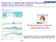
Unfortunately, it appears that the situation is often other way round: Fig. 1 presents
precipitation time series for the GATE phase III period obtained by a single–column version
of the two global models: (a) ECHAM and (b) UK UM model (as implemented into
Australian ACCESS model). In both cases, the simulated time series are much more spiky
than the observed one, suggesting that parameterizations are not working in a manner
consistent with scale separation. Thus, there are must be something wrong with the
construction of these two parameterizations. I believe that these two examples are not
exceptions. A reason for Cullen and Salmond (2003) finding that the current formulation
of convection parameterization is not compatible with a two time–scale predictor–corrector
time stepping scheme may also be partially attributed to its inconsistency with the scale
separation principle.
When a scale for a particular subgrid–scale process, say deep convection, actually
becomes closer to the grid size, i.e., ∆x → L g , one may argue that scale separation
has finally begun to break down. This is the issue to be discussed in the next section.
However, before moving to the next section, I would like to emphasize that this is not
necessarily the case, because from a point of view of asymptotic expansion (cf., Sec. 4.6),
the actual resolved scale (large–scale) of the model is still much larger than this grid
scale, i.e., ∆x → L g ≪ ∆X. Even under this regime, a very ingenious application of the
scale separation principle may better off for formulating the convection parameterization
problem, rather than pursing a one without it. This still remains an open question not
18

fully addressed.
4.9. Scale independence?
A need for a scale–independent parameterization is often claimed in context of increasing
horizontal resolutions of models. Implications that a parameterization must be
adjusted against increasing resolutions, or better still it must be constructed in such manner
than such adjustment is not at all necessary. That is roughly an idea of the scale
independence.
Here, we must realize that if a parameterization is constructed in a manner perfectly
consistent with the scale separation, it is automatically scale independent as long as the
scale separation is valid. Recall that validity of scale separation must be relatively wide
by following the arguments of Sec. 4.6.
More formally stated, under scale separation, a parameterization can be constructed
under an asymptotic expansion of a parameter, ǫ = ∆x/∆X. As long as such an asymptotic
expansion procedure is performed in formally correct manner, the resulting parameterization
must be scale independent. This conclusion does not change whether the given
parameterization explicitly includes the parameter, ǫ, or not.
Reasons for the scale dependence found in existing parameterizations mostly like come
from various ad hoc assumptions introduced without clear physical basis. These assumptions
are likely to be scale dependent, thus scrutinizing is clearly warranted. Unfortunately,
this basic issue is not much investigated.
4.10. Reality bites
Finally, reality bites. In Sec. 3.2, I have emphasized importance of a smooth solution
independent of the numerical resolution. However, such statement is valid only in a
clean problem with a well–defined large scale. Unfortunately, atmospheric flows are highly
turbulent consisting of many scales. As the numerical resolution increases, we find more
structures to be resolved. In other words, we continuously see a parameterized subgrid
scale turns into a resolved scale as the resolution increases. Under this situation, the con-
19

cept of the scale separation becomes far more subtle than otherwise, if it does not make it
useless. Refer to Sec. 4.6 again in order to recall how subtle this concept is even without
this aspect.
Occasionally, a certain phenomena, for example deep convection, crosses right at the
grid scale, L g . It is rather natural to think that we need a special attention to such a
situation, especially considering the continuous spectrum of the system. That is the issue
to be discussed in the next section.
5. Parameterization beyond Scale Separation
5.1. Background
What should we do, then, when the subgrid–scale processes no longer satisfy scale separation?
This is not merely an academic question, but the problem that many operational
research centers are facing right now as a consequence of increasing horizontal resolutions
of operational forecast models (cf., Yano et al. 2010a).
Many regional forecast models have begun to take horizontal resolutions of 1–5 km. As
a result, deep convection is almost resolved, but not quite. The standard procedure would
be to turn off deep–convection parameterization hoping that resolved model circulations
would be accurate enough to generate deep convection by themselves. Unfortunately, it
does not always happen.
Often, we face with situations in which deep convection never kicks off in spite of a
very favorable condition, and also in spite of the fact that it did kick off in validation.
In fortunate cases, we do predict deep convection but strongly localized to selective few
grid columns: a feature of grid–scale storms (e.g., Zhang et al. 1988, Molinari and Dudek
1986, 1992). For these reasons, in spite of the fact that deep convection is almost resolved,
it appears that a deep–convection parameterization is still required (cf., Kuo et al. 1997,
Bister 1998).
5.2. Conceptual issues
How can we construct a parameterization when the scale separation is no longer valid?
20

It may even be argued that the question itself is already self–contradictory.
Under the scale separation, the parameterization is a well–defined problem (in a priori
sense in spite of all the technical difficulties follow) because we have a clear distinction
between the resolved and subgrid–scale processes, given by ¯ϕ and ϕ ′ , respectively, in
Eq. (3.4). Once the scale separation is gone, there is no obvious way to distinguish what
is resolved and what is not resolved. In this respect, arguably, the parameterization ceases
to be a well–defined problem. In other words, how do we define “subgrid–scale” without
scale separation?
It is clear that if we ever want to continue to pursue the idea of parameterization
even without scale separation, we need to define “subgrid–scale” in conceptually different
way. Alternatively, a different concept other than “subgrid–scale” must be introduced for
a “parameterization”.
5.3. Mesh–refinement and nesting
The situation in concern is when, for example, deep convection is almost resolved, but
not quite. That is the issue at stake. However, obviously, if the model resolution were
slightly increased, the problem of parameterizing a particular process in concern would
simply be gone.
Diverse methods already exist in order to zoom a model in such a manner. The
stretched coordinates (cf., Baker, 1997) and adaptive mesh-refinement (AMR, e.g., Berger
and Colella 1989, Bell et al. 1994) have been traditionally adopted methods. These approaches
have been, respectively, applied to atmospheric modelling by e.g., Dietachmayer
and Droegemeier (1992) on the one hand, by e.g., Skamarock and Klemp (1993), Hubbard
and Nikiforakis (2003), Prusa and Smolarkiewicz (2003), Fournier et al. (2004),
Jablonowski et al. (2006), St-Cyr et al. (2008) on the other hand.
Nesting (e.g., Clark and Farley 1984, Zhang et al. 1986) is a more popular approach
in atmospheric modelling in order to gain higher resolutions over a local region of interest.
The basic principle of nesting resides on coupling two models with large and small domains
21

together. The procedure is easier than mesh-refinement to implement. However, due
to its design, the nesting approach tends to slave the nested–domain processes to the
host domain, completely losing its fine–scale predictability within the nested domain in
relatively short time (Laprise et al. 2008). 6) It is even harder to apply it in an adaptive
manner.
More important to keep in mind is a fact that the zooming capacity of these methods
is relatively limited, and usually it is technically possible to zoom only by factor of a few. It
is a clear distinction from multi–scale analysis introduced in Sec. 3, which is conceptually
based on the idea of “infinite” zooming by taking an asymptotic limit, ∆X/∆x → +∞.
However, such a slight zooming is exactly what we need when deep convection, for
example, is almost resolved. For this very reason, the notion of mesh–refinement and nesting
are likely to provide an important conceptual basis for developing a parameterization
when the scale separation does not exist any more.
5.4. Mass–flux based approach
It may be worthwhile to notice that the mass flux approach, outlined in Sec. 4.5, is
also based on an idea of dividing the grid box into subdomains consisting of number of
convective elements (convective plumes), as designated by Eq. (4.2), and a large remaining
part called the environment.
Under the scale separation principle, the total fractional area occupied by convective
elements is expected to be much smaller than the environment. However, arguably, this
constraint is not fundamental to the mass flux formulation. Conceptually, the basic idea
of the mass–flux formulation would relatively easily be generalized to the cases without
this constraint. Under such a generalization, any physical variable given at large–scale
6) Couple of days in their particular configuration zooming a Canadian region in a global
simulation.
22

coordinates, (X, Y ), may be given by
¯ϕ(X, Y, z, T) = ∑ j
σ j (X, Y, z, T)ϕ j (X, Y, z, T), (5.1)
where ϕ j with j = 1, 2, · · · is a value for a subgrid–scale subcomponent at (X, Y ), and σ j
is a fractional area occupied by the j–th subcomponent. Each subcomponent variable, ϕ j ,
would be described by an analogue equation to Eq. (3.9) describing the “total” large–scale
variable.
However, the above is just a very crude sketch. It would be fair to say that a precise
formulation under such a generalization is still left for debate. My own proposal is outlined
in Sec. 4 of Yano et al. (2005). A more specific application of the idea is presented in Yano
et al. (2010b). The other proposals include Gerard and Geleyn (2005), Gerard (2007),
Kuell et al. (2007). The full discussion is beyond the scope here. However, for example,
the exact position, (x j , y j ), of each subgrid–scale component is likely to become critical,
because that is no longer a matter of negligible small scales.
5.5. Stochastic approach?
On the other hand, more “statistically” based approaches such as those based on
moments are less easily modified to the cases when the scale separation breaks down.
These methods are based on the implicit assumptions that there are numerous subgrid–
scale elements over a given grid box so that a reliable statistics can be developed by
grid–scale average. Once the scale separation breaks down, these statistics are no longer
obtained in a reliable manner, because the subgrid–scale elements are no longer numerous
over the grid–box scale. 7)
If we still insist of using information from these “statistically” based approaches, the
procedure would be like taking a draw, rather than simply taking the most expected value.
Thus, an implementation would be stochastic, as an approach taken by Plant and Craig
7) Note that the argument here is exclusively focused on those half–resolved structures.
The other subgrid–scale varaibilities are not in concern of the discussions.
23

(2008, see also Plant 2010). Nevertheless, the title of their paper already indicates the
limit of their approach: it is based on an equilibrium statistics, assuming a homogeneous
background state. On the other hand, in the limit to ∆x → ∆X, the “large–scale” (or
resolved–scale) processes are expected to be highly heterogeneous to the scale even very
close the subgrid scale. In any rate, the two scales are no longer well separated, whereas
the “equilibrium” notion supposes a separation of the two.
Discussions on these limitations point to another basic character of subgrid–scale
parameterization beyond scale separation: the approach could be inherently stochastic.
5.6. Numerical Issues
It may be worthwhile to return again to certain numerical issues. As emphasized
already, “grid–point storm” is something to be avoided for stability of numerical computations.
I have already emphasized that if a parameterization is developed in a manner
consistent with the scale separation principle, “grid–point storms” should not happen.
However, once a parameterization is developed free of this principle, we no longer have a
guarantee of the absence of “grid–point storms”. Nevertheless, these are still something
to be avoided for numerical reasons. What shall we do with this situation? There are two
answers.
The first point to realize is that majority of mesh–refinement and nesting methods do
not allow us to zoom a single grid box leaving all the other neighboring grid boxes intact.
In general, both mesh–refinement and nesting must be performed over a substantial area
spanning over more than few grid boxes in one direction. Otherwise, the method would be
numerically unstable. For the same reason, zooming must be gradual in both approaches.
This argument suggests that in order to develop a legitimate subgrid–scale parameterization
without scale separation, it would be not enough to simply subdivide a given
grid–box domain as outlined under the mass–flux framework in Sec. 5.4. We also have to
carefully take into account the influences to neighboring grid boxes. In other words, lateral
interactions between grid boxes become the critical element of subgrid–scale parameteri-
24

zation under this situation.
Another way of looking at the issue is to realize that the notion of grid–box average,
that we often invoke in order to understand the idea of parameterization, does not exist
in literal sense in many numerical implementations, especially those based on either finite
difference or spectrum transform. Under these approaches, we only know the physical
values on the discretized grid, and nothing in–between by construction. We face a kind of
self–contradiction when we begin to try to subdivide a grid box in a code based on these
numerical algorithms.
A way to avoid such a self–contradiction (which may further lead to numerical instability
of the code) is to adopt a numerical algorithm that literally takes a grid box as a
basic element of computations, so that we can also take the notion of the grid box average
literally. The finite volume method developed based on this idea (cf., LeVeque 2002) could
be, thus, more desirable for constructing a high–resolution model containing subgrid–scale
parameterization without scale separation.
6. Concluding Remarks: Issues of Theories and Practice
In concluding this essay, I have to inevitably turn to the operational reality: it is often
said that there is no beautiful theory for the parameterizations. The statement reflects
a deep-rooted mentality in numerical weather forecast (NWP) community that tends to
shun theoretical approaches to parameterization.
It may be pointed out that in spite of this overall NWP mentality, there are still quite
few good theoretical works on parameterizations. A shining example is of course, Arakawa
and Schubert (1974), who also proposed the concept of the scale separation along with
many others. Most of the existing parameterizations are presented in published articles as
mathematically well–formulated systems based on theoretical ideas.
However, we have to realize that what a parameterization developer thinks what a
parameterization is doing is often not what the parameterization is actually doing. An
associated issue is a sad fact that almost no parameterization is ever implemented as
25

exactly stated in the published article even originally. The actual operational version
usually goes through various modifications that are never published in literature.
Under this situation, most people believe, we are now facing with a challenge of moving
beyond the constraint of scale separation. The intention of the present essay has been
to cast thoughts on this challenge from theoretical perspectives. Currently many stop–
gap type approaches (e.g., Gerard and Geleyn 2005, Gerard 2007, Kuell et al. 2007) are
going on in many operational research centers in order to cope with increasing horizontal
resolutions. I am also aware of the fact that many researchers are working at operational
research centers under very high pressure without much room for theoretical reflections.
On the other hand, I emphasize again the fact that current parameterizations are
constructed under the principle of scale separation. This concept is so hard wired to the
basic formulation of these parameterizations that it is more likely to mess up things if
we simply try to modify a scheme for higher resolutions without examining the whole
structure of the problem carefully. I have even suggested that a more careful construction
of a parameterization consistent with the scale separation could be a better approach under
a challenge of increasing resolutions of operational models.
The present essay is short of making any concrete proposal for parameterizations in
high–resolution limit. However, it is hoped that the present essay helps to find a way for
developing such a one by rigorous theoretical approaches.
acknowledgements
The present essay has evolved through the discussions under the COST Action ES0905.
Comments by Dmitrii Mironov, Alan L. M. Grant, Sue Gray are appreciated. The ECHAM
run shown in Fig. 1(a) is performed by Suvarchal Kumar. Greg Roff assisted me for running
the ACCESS case in Fig. 1(b).
26

References
Arakawa, A., and J.-M. Chen, 1986: Closure assumptions in the cumulus parameterization
problem. in Short– and Medium–Range Numerical Weather Prediction,
Collection of Papers at the WMO/IUGG NWP Symposium, Tokyo, 4–8 August
1986, 107–131.
Arakawa, A., and W. H. Schubert, 1974: Interaction of a cumulus cloud ensemble
with the large–scale environment, part I, J. Atmos. Sci., 31, 674–701. (AS)
Baker, T. J., 1997: Mesh Adaptation strategies for problems in fluid dynamics. Finite
Elements in Analysis and Design, 25, 243–273.
Bechtold, P., E. Bazile, F. Guichard, P. Mascart, and E. Richard, 2001: A mass-flux
convection scheme for regional and global models. Quart. J. Roy. Meteor. Soc.,
127, 869 –889.
Bell, J., M. Berger, J. Saltzman, and M. Welcome, 1994: Three-dimensional adaptive
mesh refinement for hyperbolic conservation laws. SIAM J. Sci. Comput., 15,
127–138.
Bender, C. M., and S. A. Orszag, 1978: Advanced Mathematical Methods for Scientists
and Engineers, McGraw–Hill, New York, 593pp.
Berger, M. J., and P. Colella, 1989: Local adaptive mesh refinement for shock hydrodynamics.
J. Comput. Phys., 82, 64–84.
Bister, M., 1998: Cumulus parameterisation in regional forecast models: A review;
HIRLAM Technical Report, No. 35, pp. 30.
Clark, T. L., and R. D. Farley, 1984: Severe downslope windstorm calculations in two
and three spatial dimensions using anelastic interactive grid nesting: A possible
mechanism for gustiness. J. Atmos. Sci., 41, 329–350.
Cotton, W. R., and R. A. Anthes, 1989: Storm and Cloud Dynamics. Academic Press,
880pp.
Cullen, M. J. P., and D. S. Salmond, 2003: On the use of a predictor–corrector scheme
27

to couple the dynamics with physical parameterization in the ECMWF model.
Quart. J. Roy. Meteor. Soc., 129, 127–1236.
Dietachmayer, G. S., and K. K. Droegemeier, 1992: Application of continuous dynamic
grid adaption techniques to meteorological modeling. Part I: Basic formulation
and accuracy. Mon. Wea. Rev., 120, 1675–1706.
Fournier, A., M. A. Taylor, and J. J. Tribbia, 2004: The Spectral Element Atmosphere
Model (SEAM): High-resolution parallel computation and localized resolution of
regional dynamics. Mon. Wea. Rev., 132, 726–748.
Frank, W. M., 1983: The cumulus parameterization problem. Mon. Wea. Rev., 111,
1859–1871.
Gerard, L., and J.-F. Geleyn, 2005: Evolution of a subgrid deep convection parameterization
in a limited–area model with increasing resolution. Quart. J. Roy.
Meteor. Soc., 131, 2293–2312. (GG)
Gerard, L., 2007: An integrated package for subgrid convection, clouds and precipitation
compatible with meso-gamma scales Quart. J. Roy. Meteor. Soc., 133,
711–730.
Grabowski, W. W., 2004: An improved framework for superparameterization. J.
Atmos. Sci., 61, 1940–1952.
Grabowski, W. W., 2006: Comments on “Preliminary tests of multiscale modeling
with a two–dimensional framework: Sensitivity to coupling methods”. Mon.
Wea. Rev., 134, 2012–2026.
Grabowski, W. W., and P. K. Smolarkiewicz, 1999: CRCP: A cloud resolving convection
parameterization for modeling the tropical convecting atmospehre. Physica
D, 133, 171–178.
Gyarmati, I., 1970:Non-equilirium thermodynamics. Springer, Berlin
Hubbard, M. E. and N. Nikiforakis, 2004: A three-dimensional, adaptive, Godunovtype
model for global atmospheric flows. Mon. Wea. Rev., 131, 1848–1864.
28

Jablonowski, C., M. Herzog, J. E. Penner, R. C. Oehmke, Q. F. Stout, B. van Leer,
and K. G. Powell, 2006: Block-structured adaptive grids on the sphere: Advection
experiments. Mon. Wea. Rev., 134, 3691–3713.
Kuell, V., A. Gassmann, and A. Bott, 2007: Towards a new hybrid cumulus
parametrization scheme for use in non–hydrostatic weather prediction models.
Quart. J. Roy. Meteor. Soc., 133, 479–490.
Kuo, Y., J. F. Bresch, M.–D. Cheng, J. S. Kain, D. B. Parsons, W.–K. Tao, and
D.–L. Zhang, 1997: Summary of mini workshop on cumulus parameterization for
mesoscale models. Bull. Amer. Meteor. Soc., 78, 475–491.
Lander, J. L., and B. J. Hoskins, 1997: Believable scale and parameterizations in a
spectral transform model. Mon. Wea. Rev., 125, 292–303.
Laprise, R., R. de Elia, D. Caya, S. Biner, Ph. Lucas-Picher, E. P. Diaconescu, M.
Leduc, A. Alexandru et L. Separovic, 2008: Challenging some tenets of regional
climate modelling, Meteorol. Atmos. Phys., 100, 3-22.
Leonard, A., 1974: Energy cascade in large–eddy simulations of turbulent flows. Adv.
Geophys., 418A, 237–248.
LeVeque, R. J., 2002: Finite Volume Methods for Hyperbolic Problems, Cambridge
University Press, 578pp.
Lovejoy, S., and D. Schertzer, 2010: Towards a new synthesis for atmospheric dynamics:
Space–time cascades. Atmos. Res., 96, 1–52.
Majda, A. J., 2007a: New multiscale models and self-similarity in tropical convection.
J. Atmos. Sci., 64, 1393–131404. doi:10.1175/JAS3880.1
Majda, A. J., 2007b: Multiscale models with moisture and systematic strategies for
superparameterization. J. Atmos. Sci., 64, 2726–2734.
Mapes, B. E., 1997: Equilibrium vs. activation controls on large–scale variations of
tropical deep convection. the Physics and Parameterization of Moist Atmospheric
Convection, R. K. Smith, Ed., NATO ASI, Kloster Seeon, Kluwer Academic
29

Publishers, Dordrecht, 321–358.
Meneveau, C., and J. Katz, 2000: Scale–invariance and turbulence models for large–
eddy simulation. Ann. Rev. Fluid Mech., 32, 1–32.
Mironov, D. V., 2009: Turbulence in the lower troposphere: second–order closure
and mass–flux modelling frameworks. in Interdisciplinary Aspects of Turbulence.
Lect. Notes Phys., 756, W. Hillebrandt and F. Kupka, Eds., Springer–Verlag,
Berlin, Heidelberg, 161–221. (DOI:10.1007/978–3–540–78961–1 5)
Molinari, J., and M. Dudek, 1986: Implicit versus explicit convective heating in numerical
weather prediction models. Mon. Wea. Rev., 114, 1822–1831.
Molinari, J., and M. Dudek, 1992: Parameterization of convective precipitation in
mesoscale numerical models: A critical review. Mon. Wea. Rev., 120, 326–344.
Olver, F. W. J., 1974: Asymptotics and Special Functions, Academic Press, 572pp.
Ooyama, K. V., 1982: Conceptual evolution of the theory and modeling of the tropical
cyclone, J. Met. Soc. Japan, 60, 369–380.
Pedlosky, J., 1987: Geophysical Fluid Dynamics, 2nd Ed., 710pp, Springer-Verlag.
Plant, R. S., 2010: A review of the theoretical basis for bulk mass flux convective
parameteization. Atmos. Chem. Phys., 10, 3529–3544.
Plant, R. S., and G. C. Craig, 2008: A stochastic parameterization for deep convection
based on equilibrium statistics. J. Atmos. Sci., 65, 87–105.
Prusa, J.M., and P. Smolarkiewicz, 2003: An all-scale anelastic model for geophysical
flows: Dynamic grid deformation. J. Comp. Phys., 190, 601–622.
Skamarock, W. C., and J. B. Klemp, 1993: Adaptive grid refinement for twodimensional
and three-dimensional nonhydrostatic atmospheric flow. Mon. Wea.
Rev., 121, 788–804.
St-Cyr, A., C. Jablonowski, J. M. Dennis, H. M. Tufo, and S. J. Thomas, 2008:
A comparison of two shallow water models with nonconforming adaptive grids.
Mon. Wea. Rev., 136, 1898–1922.
30

Tiedtke, M., 1989: A comprehensive mass flux scheme of cumulus parameterization
in large–scale models. Mon. Wea. Rev., 117, 1779–1800.
Tuck, A., Atmospheric Turbulence: A molecular Dynamics Perspective, Oxford University
Press.
Xing, Y., A. J. Majda, and W. W. Grabowski, 2009: New efficient sparse space–
time algorithms for superparameterization on mesoscales. J. Atmos. Sci., 137,
4307–4324.
Wyngaard, J. C., 1998: Experiment, numerical modelling, numerical simulation, and
their roles in the study of convection. in Buoyancy Convection in Geophysical
Flows, E. J. Plate, E. E. Fedorovich, D. X. Viegas, J. C. Wyngaard, Eds., pp.
239-251.
Wyngaard, J. C., 2010: Turbulence in the Atmosphere, Cambridge University Press,
393pp.
Xing, Y., A. J. Majda, and W. W. Grabowski, 2009: New efficient sparse space–
time algorithms for superparameterization on mesoscales. J. Atmos. Sci., 137,
4307–4324.
Yano, J.-I., 1992: Asymptotic theory of thermal convection in the rapidly rotating
systems, J. Fluid Mech., 243, 103-131.
Yano, J.-I., and Y. Takeuchi, 1987: The self-similarity of horizontal cloud pattern in
the intertropical convergence zone, J. Meteor. Soc. Japan, 65, 661–667.
Yano, J.-I., and N. Nishi, 1989: The hierarchy and self-affinity of the time-variability
within the tropical atmosphere inferred from the NOAA OLR data, J. Meteor.
Soc. Japan, 67, 771–789.
Yano, J.-I., W. W. Grabowski, G. L. Roff, and B. E. Mapes, 2000 : Asymptotic
approaches to convective quasi–equilibrium. Quart. J. Roy. Meteor. Soc., 126,
1861–1887.
Yano, J.-I., J.-L. Redelsperger, F. Guichard, and P. Bechtold, 2005: Mode decompo-
31

sition as a methodology for developing convective-scale representations in global
models. Quart. J. Roy. Meteor. Soc., 131, 2313–2336.
Yano, J.–I., J.–F. Geleyn, S. Malinowski, 2010a: Challenges for A New Generation
of Regional Forecast Models: Workshop on Concepts for Convective Parameterizations
in Large-Scale Model III: ”Increasing Resolution and Parameterization”;
Warsaw, Poland, 17-19 March 2010. EOS, 91, No. 26, 232.
Yano, J.-I., P. Benard, F. Couvreux, and A. Lahellec, 2010b: NAM-SCA: Nonhydrostatic
Anelastic Model under Segmentally–Constant Approximation. Mon. Wea.
Rev., 138, 1957–1974.
Zhang, D.-L., H.-R. Chang, N. L. Seaman, T. T. Warner, and J. M. Fritsch, 1986: A
two–way interactive nesting procedure with variable train resolution, Mon. Wea.
Rev., 114, 1330–1339.
Zhang, D.–L., E.–Y. Hsie, and M. W. Moncrieff, 1988: A comparison of explicit and
implicit predictions of convective and stratiform precipitating weather systems
with a meso–β–scale numerical models. Quart. J. Roy. Meteor. Soc., 114,
31–60.
32

(a) GATE Precipitation: ECHAM
(b) GATE precipitation: ACCESS
Fig. 1 : Precipitation time series for the GATE phase III period obtained by a single–
column version of the two global models: (a) ECHAM and (b) UK UM model
(as implemented into Australian ACCESS model). In (a), the observation and
the simulation are shown by the red and the black curves, respectively. In (b),
the observation and the simulation are shown by the solid and the dashed curves,
respectively.
33