Phosphorus and the Kawartha Lakes - Lakefield Herald
Phosphorus and the Kawartha Lakes - Lakefield Herald
Phosphorus and the Kawartha Lakes - Lakefield Herald

You also want an ePaper? Increase the reach of your titles
YUMPU automatically turns print PDFs into web optimized ePapers that Google loves.
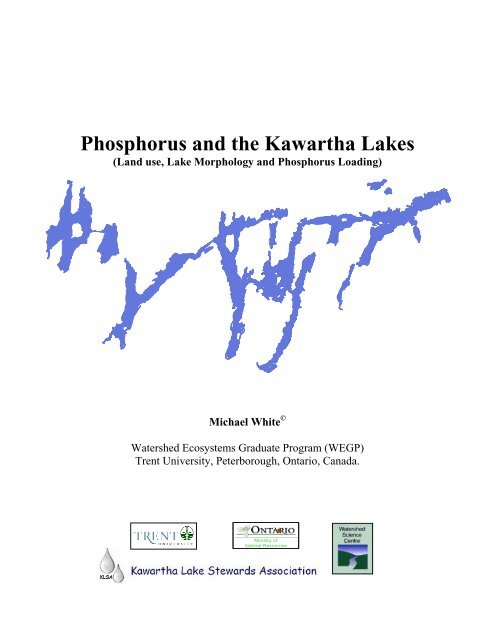
<strong>Phosphorus</strong> <strong>and</strong> <strong>the</strong> <strong>Kawartha</strong> <strong>Lakes</strong><br />
(L<strong>and</strong> use, Lake Morphology <strong>and</strong> <strong>Phosphorus</strong> Loading)<br />
Michael White ©<br />
Watershed Ecosystems Graduate Program (WEGP)<br />
Trent University, Peterborough, Ontario, Canada.<br />
Ministry of<br />
Natural Resources
Executive Summary<br />
The following document was prepared for <strong>the</strong> <strong>Kawartha</strong> Lake Stewards<br />
Association to address concerns over possible elevated phosphorus concentrations in <strong>the</strong><br />
<strong>Kawartha</strong> <strong>Lakes</strong>. The project was undertaken by Michael White (Ph.D. c<strong>and</strong>idate) in<br />
partial fulfilment of a reading course requirement (WEGP590) <strong>and</strong> supervised by Dr.<br />
Marguerite Xenopoulos. Submitted with this document is a CD containing all raw data<br />
used in <strong>the</strong> syn<strong>the</strong>sis of this report including ArcMap® files <strong>and</strong> o<strong>the</strong>r pertinent<br />
information.<br />
The development of this reading course/research was initiated by <strong>the</strong> <strong>Kawartha</strong><br />
Lake Stewards Association (KLSA). KLSA approached Trent University with concerns<br />
regarding unnatural eutrophication of <strong>the</strong>ir aquatic systems due to suspected increases in<br />
phosphorus concentrations. Using archived data, KLSA would like to know <strong>the</strong><br />
following; do lakes in <strong>the</strong>ir watersheds have higher than “normal” phosphorus<br />
concentrations, where are <strong>the</strong> areas of concern, what is <strong>the</strong> relationship of phosphorus<br />
with current watershed l<strong>and</strong> use patterns (potential sources), <strong>and</strong> recommendations for<br />
future investigations into this issue.<br />
The findings of this report (based on data mining sources) conclude that <strong>the</strong><br />
morphology of many of <strong>the</strong> <strong>Kawartha</strong> <strong>Lakes</strong>, shallow with an abundance of littoral areas,<br />
geology, located between <strong>the</strong> granitic Canadian Shield to <strong>the</strong> north <strong>and</strong> glacial till to <strong>the</strong><br />
south, along with high agricultural l<strong>and</strong> use to <strong>the</strong> south make <strong>the</strong> <strong>Kawartha</strong> <strong>Lakes</strong><br />
inherently susceptible to having above average (20-30 µg/l) phosphorus concentrations.<br />
The results found within should be viewed cautiously, as <strong>the</strong> data utilized in its syn<strong>the</strong>sis<br />
was not initially collected under a unified design; <strong>the</strong>refore, <strong>the</strong> results may prove<br />
spurious should detailed field investigations be undertaken as is suggested in <strong>the</strong><br />
conclusion of this report. All ecological studies are subject to erroneous results leaving<br />
room for misinterpretation. This report is a summation of available data on which to base<br />
direction for fur<strong>the</strong>r/future research.<br />
ii
Table of Contents<br />
EXECUTIVE SUMMARY...................................................................................... II<br />
LIST OF TABLES...................................................................................................... V<br />
LIST OF FIGURES ..................................................................................................VI<br />
1.0 INTRODUCTION ............................................................................................... 1<br />
AREA DESCRIPTION........................................................................................................ 1<br />
IMPORTANCE OF PHOSPHORUS...................................................................................... 1<br />
THE PHOSPHORUS CYCLE.............................................................................................. 1<br />
LAKE RECOVERY POTENTIAL........................................................................................ 2<br />
PROBLEM FORMULATION (WHAT ABOUT THE KAWARTHA LAKES?).......................... 3<br />
STUDY METHODOLOGY.................................................................................................. 3<br />
2.0 WATERSHED LAND CLASSIFICATION AND DELINEATION.5<br />
INTRODUCTION............................................................................................................... 5<br />
METHODOLOGY.............................................................................................................. 5<br />
RESULTS ......................................................................................................................... 5<br />
TAKE HOME MESSAGE .................................................................................................. 8<br />
3.0 PHOSPHORUS LOADING POTENTIAL ................................................ 9<br />
INTRODUCTION............................................................................................................... 9<br />
METHODOLOGY.............................................................................................................. 9<br />
RESULTS ....................................................................................................................... 10<br />
TAKE HOME MESSAGE ................................................................................................ 10<br />
4.0 LAND CLASS AND LAKE MORPHOLOGY CORRELATIONS<br />
WITH PHOSPHORUS ............................................................................................ 13<br />
INTRODUCTION............................................................................................................. 13<br />
METHODOLOGY............................................................................................................ 13<br />
RESULTS – WATERSHED ACCUMULATION.................................................................. 14<br />
RESULTS - BUFFER ....................................................................................................... 14<br />
RESULTS - LAKE MORPHOLOGY ................................................................................. 15<br />
RESULTS - MULTIPLE REGRESSION MODEL............................................................... 16<br />
CONCLUSION ................................................................................................................ 17<br />
TAKE HOME MESSAGE ................................................................................................ 17<br />
5.0 PAST AND PRESENT PHOSPHORUS LEVELS IN THE<br />
KAWARTHA LAKES ............................................................................................. 18<br />
INTRODUCTION............................................................................................................. 18<br />
METHODOLOGY............................................................................................................ 18<br />
RESULTS ....................................................................................................................... 18<br />
iii
CONCLUSION ................................................................................................................ 22<br />
TAKE HOME MESSAGE ................................................................................................ 22<br />
6.0 CONCLUSIONS ................................................................................................ 23<br />
REFERENCES ........................................................................................................... 24<br />
APPENDICES............................................................................................................. 27<br />
APPENDIX A WATERSHED LAND CLASSIFICATION ....................................................... 28<br />
APPENDIX B LAND CLASSIFICATION BUFFER (200 METERS)......................................... 32<br />
APPENDIX C STATISTICAL OUTPUT .............................................................................. 33<br />
APPENDIX D RAW DATA.............................................................................................. 53<br />
APPENDIX E BASIN CONTRIBUTION DIAGRAMS........................................................... 56<br />
APPENDIX F STREAM CONTRIBUTION MAPS................................................................ 63<br />
APPENDIX G FUTURE CONSIDERATIONS ...................................................................... 68<br />
iv
List of Tables<br />
Table 1.0 Values for spring total phosphorus <strong>and</strong> average summer chlorophyll a levels in<br />
lakes of three trophic states. Modified from Mackie (2001). .................................... 3<br />
Table 3.1 Arbitrary division of classes used in determining <strong>the</strong> phosphorus loading<br />
potential of a watershed. Modified from (Metcalfe et al., 2005)............................... 9<br />
Table 4.1 Watersheds employed in l<strong>and</strong> class/lake morphology correlations with<br />
phosphorus. See Figure 2.1 for watershed locations................................................ 14<br />
v
List of Figures<br />
Figure 2.1 NRVIS l<strong>and</strong> classification for <strong>the</strong> 31 watersheds of <strong>the</strong> <strong>Kawartha</strong> <strong>Lakes</strong><br />
region. Note that forested areas are located in <strong>the</strong> north on <strong>the</strong> Canadian Shield <strong>and</strong><br />
agricultural areas are located to <strong>the</strong> south on glacial till. Watershed Id’s are depicted<br />
in white pentagons. ..................................................................................................... 6<br />
Figure 2.2 PCA ordination of Watershed characterization. Note <strong>the</strong> majority of <strong>the</strong><br />
separation is along Axis 1, which demonstrates a clear distinction between forested<br />
<strong>and</strong> agricultural l<strong>and</strong>scapes. Vector length is proportionate to it influence on site<br />
separation. This shows graphically <strong>the</strong> same separation that is shown visually from<br />
a l<strong>and</strong> classification map (Figure 2.1). The dashed orange line present in <strong>the</strong><br />
ordination (left) is transposed on <strong>the</strong> watershed schematic (right) <strong>and</strong> demonstrates<br />
that <strong>the</strong> PCA separation in l<strong>and</strong> use is synonymous with <strong>the</strong> visual separation shown<br />
in a l<strong>and</strong> use map. The dashed orange line also represents areas where limestone<br />
alvar plain habitat can be found.................................................................................. 7<br />
Figure 3.1 Quaternary watershed phosphorus susceptibility in Sou<strong>the</strong>rn Ontario.<br />
<strong>Kawartha</strong> <strong>Lakes</strong> watersheds are outlined in black. Base picture taken from<br />
(Metcalfe et al., 2005)............................................................................................... 11<br />
Figure 3.2 <strong>Phosphorus</strong> susceptibility for <strong>the</strong> 31 quaternary watersheds of <strong>the</strong> <strong>Kawartha</strong><br />
lakes. Susceptibility is determined through modeled base flow <strong>and</strong> percent<br />
agricultural l<strong>and</strong>scape. Note, water entering <strong>the</strong> <strong>Kawartha</strong> <strong>Lakes</strong> from sou<strong>the</strong>rn<br />
catchments is more likely to have higher phosphorus concentrations. Watershed Id’s<br />
can be found on page 6 in Figure 2.1........................................................................ 12<br />
Figure 4.1 Linear regression of total phosphorus with proportion of watershed l<strong>and</strong><br />
classifications for; a) freshwater marsh, b) coniferous swamp, c) open fen, d) pasture<br />
<strong>and</strong> ab<strong>and</strong>oned fields, e) coniferous plantation, f) mixed forest mostly deciduous, g)<br />
cropl<strong>and</strong>, h) mean lake depth, i) settlement <strong>and</strong> developed l<strong>and</strong>. <strong>Phosphorus</strong><br />
concentrations are calculated from mean August 2005 values (N = 9). ................... 15<br />
Figure 4.2 Multiple regression predictive model of phosphorus concentrations<br />
constructed using <strong>the</strong> following four environmental predictors; mean depth,<br />
freshwater marsh, pasture/ab<strong>and</strong>oned fields, <strong>and</strong> cropl<strong>and</strong>. Dashed lines delineate<br />
95% confidence intervals.......................................................................................... 16<br />
Figure 5.1 Bar graph showing mean August total phosphorus concentrations <strong>and</strong><br />
st<strong>and</strong>ard deviations for ten <strong>Kawartha</strong> lakes (Balsam, Big Bald, Upper Buckhorn,<br />
Cameron, Clear, Katchewanooka, Pigeon, Sturgeon, Upper <strong>and</strong> Lower Stony) for<br />
1972, 1976 <strong>and</strong> 2005. Different letters denote significant differences between<br />
means following ANOVA procedure <strong>and</strong> Tukey’s test (p = 0.001)(N=10). ............ 19<br />
vi
Figure 5.2 Linear regression of August total phosphorus concentrations across years for<br />
Sturgeon lake from a) 1971-1991, N = 21, b) 1971-2005, N = 24. Note, it appears<br />
phosphorus concentrations have remained relatively constant since 1988............... 19<br />
Figure 5.3 Spline curve of seven <strong>Kawartha</strong> <strong>Lakes</strong> along a down stream/lake gradient<br />
from Balsam Lake to Katchewanooka Lake. <strong>Phosphorus</strong> levels are pooled August<br />
concentrations <strong>and</strong> patterns should be interpreted cautiously as sample intensity<br />
varies greatly between years <strong>and</strong> lakes. .................................................................... 20<br />
Figure 5.4 Lake chain outline overlaid by a non-linear regression (logistic, 3 parameter,<br />
solid black line) of mean August 2005 phosphorus concentrations with lake position.<br />
Lake position is defined as 1 plus <strong>the</strong> number of lakes that eventually feed into it.<br />
<strong>Lakes</strong> used in analyses are ei<strong>the</strong>r part of <strong>the</strong> Trent Severn Waterway or contribute to<br />
it. Water flows form Balsam Lake (left) through to Katchewanooka Lake (right).<br />
Dotted line represents a plausible repetition of <strong>the</strong> logistic pattern after <strong>the</strong> dilution<br />
<strong>and</strong> resultant decrease in phosphorus concentration has occurred from <strong>the</strong><br />
confluence of Upper Stony Lake <strong>and</strong> Lovesick Lake at Burleigh Falls. .................. 21<br />
vii
1.0 Introduction<br />
Area Description<br />
The <strong>Kawartha</strong> <strong>Lakes</strong> watershed contains 31 sub-watersheds <strong>and</strong> covers an area of<br />
approximately 8,990 km 2 . It contains numerous lakes, many of <strong>the</strong> largest form part of<br />
<strong>the</strong> Trent Severn Waterway. The sou<strong>the</strong>rn half of <strong>the</strong> watershed is dominated by glacial<br />
till <strong>and</strong> littered with drumlins <strong>and</strong> of course <strong>the</strong> Oak Ridges Moraine. The nor<strong>the</strong>rn half<br />
of <strong>the</strong> watershed is predominantly Canadian Shield <strong>and</strong> is <strong>the</strong> start of “cottage country”.<br />
For a detailed history <strong>and</strong> description of <strong>the</strong> study area please see THE KAWARTHA<br />
LAKES (Walters, 2006).<br />
Importance of <strong>Phosphorus</strong><br />
Human induced nutrient enrichment, or eutrophication, of aquatic ecosystems has<br />
been <strong>the</strong> focus of much research over <strong>the</strong> past two decades (Beasley et al., 1985; Hart et<br />
al., 2004; Makarewicz <strong>and</strong> Bertram, 1991; Schindler et al., 1971; Sims et al., 1998).<br />
Even though o<strong>the</strong>r nutrients are associated with eutrophication, phosphorus is of major<br />
concern as it is usually <strong>the</strong> most limiting nutrient in freshwater ecosystems (Schindler,<br />
1977). The relationship between lake eutrophication (nutrient loading) <strong>and</strong><br />
phytoplankton abundance became common knowledge about 30 years ago (Schindler,<br />
1987; Vollenweider, 1976) <strong>and</strong> we now underst<strong>and</strong> that lakes are subject to regime shifts<br />
from clear macrophyte dominated systems to turbid phytoplankton dominated systems<br />
(Bayley <strong>and</strong> Pra<strong>the</strong>r, 2003; Genkai-Kato <strong>and</strong> Carpenter, 2005). The driving force behind<br />
<strong>the</strong> clear to turbid shift is elevated phosphorus concentrations (Delerck et al., 2005;<br />
Jeppesen et al., 2005; Portielje <strong>and</strong> Rijsdijk, 2003). The elevated phosphorus<br />
concentrations correspond to increased phytoplankton production (Table 1.1).<br />
The <strong>Phosphorus</strong> Cycle<br />
<strong>Phosphorus</strong> is found in both soluble <strong>and</strong> insoluble forms, which toge<strong>the</strong>r account<br />
for <strong>the</strong> total phosphorus (TP) in a lake ecosystem. The insoluble forms occur<br />
predominantly from dead or decaying organisms (leaf litter, aquatic macrophytes,<br />
phytoplankton, zooplankton, etc.) <strong>and</strong> eventually falls to <strong>the</strong> lake bottom, while <strong>the</strong><br />
soluble forms stay suspended in <strong>the</strong> lake water column. Soluble phosphorus is comprised<br />
of numerous complex compounds; however, a proportion is soluble reactive phosphorus<br />
(SRP). SRP is readily used (absorbed) by phytoplankton <strong>and</strong> macrophytes <strong>and</strong> thus<br />
increases lake productivity. Almost all natural sources of phosphorus (~90%) enter a<br />
lake system in <strong>the</strong> insoluble form, whereas, phosphorus from anthropogenic (human<br />
induced) sources are predominately of <strong>the</strong> soluble form (~90%) (Mackie, 2001). This<br />
means that phosphorus entering aquatic systems from human sources is immediately<br />
available for primary production. The insoluble phosphorus, which has fallen to <strong>the</strong> lake<br />
sediment, can be converted to soluble form <strong>and</strong> is not trapped <strong>the</strong>re permanently. The<br />
1
mobilization process can be quite complex, but in its simplest form insoluble phosphorus<br />
can be reduced to a soluble state at <strong>the</strong> sediment-water interface through decreasing redox<br />
potential <strong>and</strong> pH levels. These conditions exist when lake sediment oxygen levels<br />
decrease <strong>and</strong> become anoxic (depleted of oxygen). This anoxic condition occurs in lakes<br />
when algae die <strong>and</strong> fall to <strong>the</strong> lake bottom. As <strong>the</strong> dead algae are decomposed bacteria<br />
consume oxygen <strong>and</strong> favourable conditions for phosphorus mobilization occur (Mackie,<br />
2001). Thus, once a lake becomes eutrophic (turbid algal state) this negative feedback<br />
loop can make restoration efforts challenging.<br />
So what does this tell us? It is possible to limit anthropogenic sources of<br />
phosphorus, creating an initial decrease in levels; however, long-term reduction may take<br />
many years as <strong>the</strong> insoluble phosphorus is mobilized <strong>and</strong> absorbed by plant species. The<br />
easiest way to restore a lake is to prevent it from becoming eutrophic in <strong>the</strong> first place.<br />
Recent studies suggest that <strong>the</strong> degree <strong>and</strong> rate at which a lake can reduce its phosphorus<br />
concentration depends on many factors; <strong>the</strong>se are discussed in <strong>the</strong> following section.<br />
Lake Recovery Potential<br />
The undesirable phenomenon of lake eutrophication has lead to many restoration<br />
efforts. Current research has been devoted to discovering <strong>the</strong> underling drivers in <strong>the</strong> reoligotrophication<br />
process. Søndergaard et al. (2005) conducted an excellent study of 12<br />
lakes in Denmark to determine lake response to reduced nutrient loads. Their findings<br />
demonstrate that internal loading of phosphorus can significantly delay lake recovery (up<br />
to 10 years) <strong>and</strong> that lake morphology (shallow vs. deep basins) must also be considered<br />
in restoration efforts. The shallow basins do not stratify (have one <strong>the</strong>rmal layer) <strong>and</strong> are<br />
subject to more wave action <strong>the</strong>reby altering phosphorus resuspension <strong>and</strong><br />
remobilization. A similar study by Jeppesen et al. (2005), which incorporated <strong>the</strong> same<br />
Danish lakes into a larger data set of 35 case studies, had similar conclusions concerning<br />
reduced nutrient loading. They found that internal loading delayed lake recovery; lower<br />
phosphorus levels did not stabilize until 10-15 years had past. Interestingly, fish biomass<br />
was found to decline in <strong>the</strong> majority of cases; however, piscivorous (fish that eat o<strong>the</strong>r<br />
fish) increased in 80% of <strong>the</strong> case studies. Phytoplankton community structure reverted<br />
back to oligotrophic species, but submerged macrophyte communities reappeared in only<br />
50% of <strong>the</strong> lakes for which data was available. As Declerck et al. (2005) point out,<br />
phosphorus can both directly <strong>and</strong> indirectly affect aquatic diversity. It can act directly on<br />
plants, which absorb it, or indirectly through changes in macrophyte communities<br />
creating habitat <strong>and</strong> refuge for fish <strong>and</strong> zooplankton.<br />
Two of <strong>the</strong> most important factors controlling lake response to reduced nutrient<br />
loads are mean depth (calculated as <strong>the</strong> lake volume divided by its surface area) <strong>and</strong><br />
macrophyte abundance (Genkai-Kato <strong>and</strong> Carpenter, 2005). Curiously, <strong>the</strong> lakes most<br />
resistant in recovering to a clear state are lakes of intermediate size. These problematic<br />
lakes have a mean depth around 10 meters. They are too deep to be aided by<br />
macrophytes (which decrease water turbidity by acting as nutrient traps, thus limiting <strong>the</strong><br />
resuspension of sediment material <strong>and</strong> negatively affecting algal growth (Portielje <strong>and</strong><br />
Rijsdijk, 2003)) <strong>and</strong> too shallow to mitigate internal phosphorus loading through dilution<br />
in <strong>the</strong> hypolimnion (Genkai-Kato <strong>and</strong> Carpenter, 2005). This suggests that some of <strong>the</strong><br />
2
<strong>Kawartha</strong> <strong>Lakes</strong> may not be able to revert to a clear state once a shift to a turbid algal<br />
dominated one has occurred.<br />
Table 1.0 Values for spring total phosphorus <strong>and</strong> average summer chlorophyll a levels in<br />
lakes of three trophic states. Modified from Mackie (2001).<br />
Trophic State Total <strong>Phosphorus</strong> µg/L Chlorophyll a<br />
Oligotrophic (Clear water) < 10 < 2<br />
Mesotrophic 10 – 20 2 – 5<br />
Eutrophic (Turbid water) > 30 > 5<br />
Problem Formulation (What about <strong>the</strong> <strong>Kawartha</strong> <strong>Lakes</strong>?)<br />
Of <strong>the</strong> many anthropogenic (human induced) sources of phosphorus four are<br />
likely to be <strong>the</strong> significant contributors to <strong>the</strong> <strong>Kawartha</strong> <strong>Lakes</strong> phosphorus levels;<br />
agriculture (fertilizer runoff), faulty septic systems, urban runoff, <strong>and</strong> wastewater<br />
treatment facilities. Historical anthropogenic inputs of phosphorus to sediments are also<br />
likely in <strong>the</strong> <strong>Kawartha</strong> <strong>Lakes</strong> watershed along with many o<strong>the</strong>r natural <strong>and</strong> unnatural<br />
sources but <strong>the</strong>se would be extremely difficult, if not impossible, to reduce. <strong>Phosphorus</strong><br />
loading by invasive animal populations is also a concern. Emerging evidence suggest<br />
that dreissenids (Zebra mussels) can negatively affect phosphorus cycling within lakes<br />
(Hecky et al., 2004). It has been postulated that <strong>the</strong> dreissenids retain phosphorus in<br />
nearshore areas where it can accumulate <strong>and</strong> may be linked with <strong>the</strong> nuisance filamentous<br />
green algae Cladophora. Dreissenids invasions in <strong>the</strong> <strong>Kawartha</strong> <strong>Lakes</strong> could be<br />
contributing to <strong>the</strong>ir high macrophyte (aquatic plants) abundances by filtering<br />
phytoplankton (<strong>and</strong> <strong>the</strong> phosphorus contained in <strong>the</strong>m) <strong>and</strong> depositing it as pseudo-feces<br />
onto <strong>the</strong> lake bottom. This causes a reduction of phosphorus concentrations in open<br />
water areas but conversely increases concentrations in <strong>the</strong> sediment-water interface <strong>and</strong><br />
littoral (nearshore) areas. Similar to dreissenids, <strong>the</strong>re is evidence that geese can<br />
significantly elevate nutrient levels (Olson et al., 2005), this may be a problem in <strong>the</strong><br />
<strong>Kawartha</strong> lakes area if populations are high.<br />
The <strong>Kawartha</strong> Lake Stewards Association (KLSA) is concerned about <strong>the</strong><br />
phosphorus levels in <strong>the</strong>ir region. The reason for this concern is that phosphorus levels<br />
are currently around 17 µg/L <strong>and</strong> it is possible that a concentration of > 20 µg/L may lead<br />
to foul-smelling algal blooms <strong>and</strong> a shift towards a turbid algae dominated lake system<br />
(KLSA, 2005). Should a shift in lake regime to a turbid system occur it would be<br />
difficult <strong>and</strong> costly, if not impossible, to remediate. The following pages are a summary<br />
of archived data with which to assess <strong>the</strong> history, patterns <strong>and</strong> possible sources of<br />
phosphorus in <strong>the</strong> <strong>Kawartha</strong> <strong>Lakes</strong>.<br />
Study Methodology<br />
The first step in assessing phosphorus levels is to assemble all historical data for<br />
<strong>the</strong> lakes of concern. The data contained in this report were primarily acquired through<br />
past studies conducted by <strong>the</strong> Ministry of <strong>the</strong> Environment (MOE) (Hutchinson et al.,<br />
3
1994; MOE, 1976), Ministry of Natural Resources (MNR) (Hutchinson et al., 1994),<br />
KLSA (KLSA, 2006), MOE’s Lake Research Partner program (MOE, 2006) <strong>and</strong> <strong>the</strong><br />
Ministry of Natural Resources (MNR) Natural Resources Values <strong>and</strong> Information System<br />
(NRVIS) data base (MNR, 2002).<br />
Using a combination of statistical techniques, regression (Sigma Plot©, Jump©),<br />
ordination (PC-ORD©), <strong>and</strong> analyses of variance (ANOVA)(Jump©) archived data will<br />
be utilized to address <strong>the</strong> following questions:<br />
1. What are <strong>the</strong> l<strong>and</strong> use characteristics of <strong>the</strong> <strong>Kawartha</strong> <strong>Lakes</strong> watersheds?<br />
2. Is l<strong>and</strong> use correlated with phosphorus concentrations in lakes within <strong>the</strong><br />
<strong>Kawartha</strong> <strong>Lakes</strong> watershed?<br />
3. What lake morphological variables are correlated with phosphorus<br />
concentrations?<br />
4. Have phosphorus levels been increasing or decreasing in <strong>the</strong> lakes within <strong>the</strong><br />
<strong>Kawartha</strong> <strong>Lakes</strong> watershed?<br />
5. What patterns in lake phosphorus concentrations can be determined from <strong>the</strong><br />
archived data?<br />
The chapters that follow will help elucidate <strong>the</strong>se questions <strong>and</strong> provide insight into<br />
<strong>the</strong> complex relationships of phosphorus in <strong>the</strong> <strong>Kawartha</strong> <strong>Lakes</strong>.<br />
4
2.0 Watershed L<strong>and</strong> Classification <strong>and</strong> Delineation<br />
Introduction<br />
The first step in determining l<strong>and</strong> use relationships with lake phosphorus<br />
concentrations is establishing where <strong>and</strong> what kinds of l<strong>and</strong> use are prevalent. This first<br />
chapter is devoted to determining both, <strong>the</strong> quantity <strong>and</strong> location of quaternary (MNRs<br />
most detailed watershed delineation) watersheds, <strong>and</strong> <strong>the</strong> l<strong>and</strong> use within each.<br />
Methodology<br />
Ontario’s NRVIS database (MNR, 2002) <strong>and</strong> <strong>the</strong> Water Resources <strong>and</strong><br />
Information Project (WRIP)(MNR, 2006) were utilized to acquire l<strong>and</strong> class information<br />
<strong>and</strong> watershed delineations. These datum were <strong>the</strong>n overlaid <strong>and</strong> analysed using<br />
ArcMap® to determine watershed boundaries <strong>and</strong> <strong>the</strong> l<strong>and</strong> uses within <strong>the</strong>m.<br />
Results<br />
It was found that <strong>the</strong> <strong>Kawartha</strong> <strong>Lakes</strong> watershed (8,990 km 2 ) consists of 31<br />
quaternary watersheds. As seen in Figure 2.1, of <strong>the</strong> possible 28 l<strong>and</strong> uses identified by<br />
<strong>the</strong> NRVIS datum <strong>the</strong> <strong>Kawartha</strong> <strong>Lakes</strong> Watershed is represented by 21 different l<strong>and</strong><br />
uses. Interestingly, <strong>the</strong> chain of lakes running West/East through <strong>the</strong> middle of <strong>the</strong><br />
watershed (Trent Severn Waterway) run parallel with a transition zone between forested<br />
Canadian Shield (metamorphosed limestone <strong>and</strong>/or granite) catchments to <strong>the</strong> north <strong>and</strong><br />
agricultural glacial till catchments to <strong>the</strong> south. This transition zone includes a significant<br />
limestone alvar plain that runs through <strong>the</strong> <strong>Kawartha</strong> <strong>Lakes</strong> watershed. Principal<br />
Components Analysis (PCA) demonstrates a clear gradient between forested <strong>and</strong><br />
agricultural catchments (Figure 2.2). Exact watershed areas <strong>and</strong> percent l<strong>and</strong><br />
classifications for each of <strong>the</strong> 31 watersheds are located in appendix A.<br />
5
IJ 2 IJ 18 IJ 5<br />
IJ 1<br />
IJ 3<br />
Legend<br />
IJ 4 IJ 20<br />
Water<br />
FreshwaterMarsh<br />
Deciduous Swamp<br />
ConiferSwamp<br />
open fen<br />
open bog<br />
treed bog<br />
dense deciduous<br />
dense coniferous<br />
coniferous plantation<br />
mixed deciduous<br />
mixed coniferous<br />
sparse coniferous<br />
sparse deciduous<br />
recent cutover<br />
bedrock/s<strong>and</strong>/gravel<br />
settlement<br />
pasture <strong>and</strong> ab<strong>and</strong>oned fields<br />
cropl<strong>and</strong><br />
alvar<br />
unclassified<br />
IJ 6 IJ 14<br />
IJ 12<br />
17 IJ 21<br />
IJ 29<br />
IJ 7 IJ 9<br />
IJ 11<br />
IJ 10<br />
IJ 23<br />
IJ 16 IJ 15<br />
IJ 24 IJ 25<br />
IJ 19 IJ<br />
IJ 22<br />
IJ<br />
IJ 27<br />
IJ 30<br />
IJ 31 IJ 8<br />
Peterborough<br />
4.5<br />
{Kilometers<br />
IJ 13 IJ 26 0 9 18 27 36<br />
Figure 2.1 NRVIS l<strong>and</strong> classification for <strong>the</strong> 31 watersheds of <strong>the</strong> <strong>Kawartha</strong> <strong>Lakes</strong> region. Note that forested areas are located in <strong>the</strong><br />
north on <strong>the</strong> Canadian Shield <strong>and</strong> agricultural areas are located to <strong>the</strong> south on glacial till. Watershed Id’s are depicted in white<br />
pentagons.<br />
6
1<br />
Dense Deciduous<br />
3<br />
2<br />
1<br />
Axis 1<br />
15B<br />
16A<br />
2<br />
20<br />
18A<br />
2<br />
23<br />
4<br />
Recent Cutover<br />
16B<br />
28<br />
13<br />
Open Water<br />
5<br />
7<br />
Sparse Deciduous<br />
Pasture<br />
Conifer Swamp<br />
8<br />
Mixed Coniferous<br />
Cropl<strong>and</strong><br />
-4 0 Treed 4<br />
Bog<br />
Deciduous Swamp<br />
12<br />
Mixed Deciduous<br />
30<br />
6<br />
14<br />
22<br />
Open Bog<br />
Sparse Coniferous<br />
10<br />
17B<br />
29<br />
Unclassified<br />
31<br />
-2<br />
15A<br />
9<br />
30<br />
4<br />
6<br />
7<br />
13<br />
16<br />
19<br />
26<br />
25<br />
11<br />
12<br />
29<br />
31<br />
28<br />
5<br />
9<br />
10<br />
18<br />
22<br />
15<br />
14<br />
20<br />
21<br />
27<br />
19B<br />
21<br />
25<br />
26<br />
24<br />
17A<br />
19A<br />
18B<br />
27<br />
-6<br />
Axis 2<br />
11<br />
Figure 2.2 PCA ordination of Watershed characterization. Note <strong>the</strong> majority of <strong>the</strong> separation is along Axis 1, which demonstrates a<br />
clear distinction between forested <strong>and</strong> agricultural l<strong>and</strong>scapes. Vector length is proportionate to it influence on site separation. This<br />
shows graphically <strong>the</strong> same separation that is shown visually from a l<strong>and</strong> classification map (Figure 2.1). The dashed orange line<br />
present in <strong>the</strong> ordination (left) is transposed on <strong>the</strong> watershed schematic (right) <strong>and</strong> demonstrates that <strong>the</strong> PCA separation in l<strong>and</strong> use<br />
is synonymous with <strong>the</strong> visual separation shown in a l<strong>and</strong> use map. The dashed orange line also represents areas where limestone<br />
alvar plain habitat can be found.<br />
7
Take Home Message<br />
Previous models of lake phosphorus concentrations <strong>and</strong> catchment related<br />
phosphorus dynamics would be problematic if applied to <strong>the</strong> <strong>Kawartha</strong> <strong>Lakes</strong> area. This<br />
is due to <strong>the</strong> unique situation of having lakes located between two extreme geological<br />
features combined with unusually shallow lake systems (most have artificially high water<br />
levels due to dam creation for <strong>the</strong> Trent Severn Waterway, this causes <strong>the</strong> historical<br />
floodplain to be inundated with water, which decrease mean depth <strong>and</strong> increases littoral<br />
habitats where macrophytes can proliferate). The l<strong>and</strong>scape to <strong>the</strong> south of <strong>the</strong> <strong>Kawartha</strong><br />
<strong>Lakes</strong> is dominated by cultivated l<strong>and</strong> with glacial till, while <strong>the</strong> area to <strong>the</strong> north is<br />
dominated by forested areas <strong>and</strong> impermeable bedrock.<br />
8
3.0 <strong>Phosphorus</strong> Loading Potential<br />
Introduction<br />
The eutrophication of aquatic systems has been a known phenomenon for many<br />
years <strong>and</strong> much research has been undertaken to predict <strong>the</strong> potential influence of l<strong>and</strong><br />
use on aquatic phosphorus loading. An excellent application of this research in sou<strong>the</strong>rn<br />
Ontario predicts <strong>the</strong> phosphorus-loading potential of a watershed based on base flow<br />
(minimum amount of water available to streams) <strong>and</strong> cropl<strong>and</strong>. More details on <strong>the</strong><br />
model can be found online <strong>and</strong> should be consulted to fully underst<strong>and</strong> this chapter<br />
(Metcalfe et al., 2005).<br />
Methodology<br />
The predictive model utilized in this chapter is a direct application of research<br />
conducted by Metcalfe et al. (2005) <strong>and</strong> assigns a value to a watershed based on its<br />
potential to contribute phosphorus to watercourses. The values range from 1 – 15, with 1<br />
having a low potential to contribute phosphorus <strong>and</strong> 15 having <strong>the</strong> highest potential. This<br />
scale was developed after analysing real data from thirteen reference watersheds scattered<br />
from Kitchener, ON, to Cornwall, ON. The model incorporates <strong>the</strong> Base Flow Index<br />
(BFI) <strong>and</strong> percent cropl<strong>and</strong> for a watershed to calculate its phosphorus loading potential<br />
(Table 3.1). It <strong>the</strong>n applies <strong>the</strong> equation:<br />
<strong>Phosphorus</strong> Susceptibility Index = (% Cropl<strong>and</strong> Class – BFI Class) + 8<br />
Thus, once you figure out <strong>the</strong> % Cropl<strong>and</strong> <strong>and</strong> BFI value of a watershed (using<br />
available government provided geospatial l<strong>and</strong>scape datum) you can predict its<br />
phosphorus loading potential.<br />
Table 3.1 Arbitrary division of classes used in determining <strong>the</strong> phosphorus loading<br />
potential of a watershed. Modified from (Metcalfe et al., 2005).<br />
Class % Cropl<strong>and</strong> Class Upper boundary BFI (%)<br />
1 32.5 1 0.124<br />
2 50.7 2 0.202<br />
3 63.4 3 0.28<br />
4 73.2 4 0.358<br />
5 81.8 5 0.436<br />
6 87.8 6 0.514<br />
7 93.6 7 0.592<br />
8 100 8 1<br />
9
Results<br />
Although <strong>the</strong> <strong>Kawartha</strong> <strong>Lakes</strong> watershed has a relatively low phosphorus loading<br />
potential when compared to <strong>the</strong> majority of sou<strong>the</strong>rn Ontario, Figure 3.1, it is unique in<br />
that it has an altered waterway (permanently flooded historical flood plain) with which to<br />
concentrate its nutrient loading. The 31 quaternary watersheds had percent cropl<strong>and</strong><br />
classes between 1 <strong>and</strong> 3, <strong>and</strong> BFI classes between 4 <strong>and</strong> 8. This resulted in a range of<br />
phosphorous susceptibility index values from 1 to7. Comparable to <strong>the</strong> l<strong>and</strong> classification<br />
results in chapter 2, we see a distinct separation along <strong>the</strong> chain of lakes, with low<br />
phosphorus loading potential to <strong>the</strong> north <strong>and</strong> high loading potential to <strong>the</strong> south (Figure<br />
3.2). This model predicts that <strong>the</strong> sou<strong>the</strong>rn watersheds will contribute more phosphorus<br />
to <strong>the</strong> <strong>Kawartha</strong> <strong>Lakes</strong> than <strong>the</strong> nor<strong>the</strong>rn watersheds.<br />
Take Home Message<br />
This model should be interpreted with caution as it does not take into account<br />
o<strong>the</strong>r morphological variables (i.e. shallow lakes, drainage basin ratio) that may<br />
compound <strong>the</strong> phosphorus loading issue. Although <strong>the</strong>re are many factors that can<br />
contribute phosphorus to a watershed; sewage treatment plants, aerial deposition, faulty<br />
septic systems <strong>and</strong> animal feces (beef, poultry, hog operations <strong>and</strong> large populations of<br />
geese <strong>and</strong> zebra mussels), clearly arable l<strong>and</strong> plays an important component in elevating<br />
phosphorus concentrations in water bodies.<br />
10
<strong>Kawartha</strong> lakes watershed<br />
IJ 2 IJ 18 IJ 5<br />
IJ 1<br />
IJ 3<br />
IJ 4 IJ 20<br />
IJ 8<br />
IJ 6<br />
IJ 7 IJ 9<br />
IJ IJ IJ11<br />
10<br />
14<br />
IJ 12<br />
IJ<br />
IJ 15<br />
16 IJ 19 IJ 17 IJ 23 IJ 21<br />
IJ IJ 24<br />
25<br />
IJ 22<br />
IJ 29<br />
IJ<br />
IJ 27<br />
IJ IJ 30<br />
31 28<br />
4.5<br />
{Kilometers<br />
IJ 13 IJ 26 0 9 18 27 36<br />
Figure 3.1 Quaternary watershed phosphorus susceptibility in Sou<strong>the</strong>rn Ontario. <strong>Kawartha</strong> <strong>Lakes</strong> watersheds are outlined in black.<br />
Base picture taken from (Metcalfe et al., 2005).<br />
11
1<br />
1<br />
1<br />
1<br />
1<br />
2<br />
1<br />
1<br />
1<br />
1<br />
1<br />
1<br />
1<br />
1<br />
1<br />
1<br />
Lambertstudya<br />
Phosphorous Susceptibility Index<br />
suscept.SUSCEPTABI<br />
1<br />
3<br />
4<br />
4<br />
3<br />
4<br />
1<br />
3<br />
2<br />
2<br />
3<br />
2<br />
3<br />
4<br />
5<br />
6<br />
7<br />
5<br />
7<br />
3<br />
7 6<br />
4<br />
4<br />
3<br />
3<br />
{<br />
0 5<br />
10 20 30 40<br />
Kilometers<br />
Figure 3.2 <strong>Phosphorus</strong> susceptibility for <strong>the</strong> 31 quaternary watersheds of <strong>the</strong> <strong>Kawartha</strong> lakes. Susceptibility is determined through<br />
modeled base flow <strong>and</strong> percent agricultural l<strong>and</strong>scape. Note, water entering <strong>the</strong> <strong>Kawartha</strong> <strong>Lakes</strong> from sou<strong>the</strong>rn catchments is more<br />
likely to have higher phosphorus concentrations. Watershed Id’s can be found on page 6 in Figure 2.1.<br />
12
4.0 L<strong>and</strong> Class <strong>and</strong> Lake Morphology Correlations with <strong>Phosphorus</strong><br />
Introduction<br />
Chapter 4 focuses on one of <strong>the</strong> major goals of this report, which was to utilize<br />
<strong>the</strong> NRVIS database (outlined in chapter 1) to determine what relationships exist between<br />
l<strong>and</strong> use <strong>and</strong> phosphorus concentrations in <strong>the</strong> <strong>Kawartha</strong> <strong>Lakes</strong>; as nutrient<br />
concentrations in watercourses have often been attributed to <strong>the</strong> l<strong>and</strong> use activities<br />
inhabiting <strong>the</strong>m (Beasley et al., 1985; Cooke <strong>and</strong> Prepas, 1998). A second focus was to<br />
resolve any relationships that phosphorus concentrations may demonstrate with lake<br />
morphology, similar to findings in o<strong>the</strong>r geographic areas (Genkai-Kato <strong>and</strong> Carpenter,<br />
2005).<br />
Methodology<br />
Multiple linear regression analyses were employed to determine <strong>the</strong> relationship<br />
between phosphorus concentrations <strong>and</strong> l<strong>and</strong> use/lake morphology characteristics. The<br />
“dependant” variable phosphorus was tested for a linear relationship with each<br />
“independent” l<strong>and</strong> use/lake morphology variable. L<strong>and</strong> use information was ga<strong>the</strong>red<br />
from <strong>the</strong> NRVIS database, lake morphology information from <strong>the</strong> MNR’s lake database,<br />
<strong>and</strong> phosphorus concentrations were mean August 2005 values taken from KLSA’s<br />
dataset. Three analyses were preformed to test for linearity with phosphorus<br />
concentrations: increasing watershed contributions, lake buffer of l<strong>and</strong> use (200 m), <strong>and</strong><br />
lake morphology. In order to test <strong>the</strong> relationship of watershed accumulation with<br />
phosphorus concentration it was necessary to establish which watersheds contribute to<br />
each particular lake. Table 4.1, outlines watershed contributions for each of <strong>the</strong> nine<br />
lakes used in analyses. The following nine lakes were <strong>the</strong> sole lakes with suitable datum<br />
for both <strong>the</strong> watershed l<strong>and</strong> use analysis <strong>and</strong> lake morphology analysis; Big Bald, Upper<br />
Stony, Balsam, Cameron, Sturgeon, Pigeon, Upper Buckhorn, Lovesick, <strong>and</strong><br />
Katchewanooka <strong>Lakes</strong>. Similarly, surrounding l<strong>and</strong> use, from shore to 200m, was<br />
calculated for each lake using ArcMap®; see appendix B for exact values. A two<br />
hundred meter buffer was used as most literature emphasises that a 100-300m buffer is<br />
effective at alleviating nutrient runoff <strong>and</strong> to incorporate <strong>the</strong> effect of shoreline<br />
development. Eleven lakes had suitable datum for <strong>the</strong> 200m lake buffer analysis; Upper<br />
Stony, Upper Buckhorn, Sturgeon, Pigeon, Lovesick, Lower Stony, Katchewanooka,<br />
Chemong, Cameron, Big Bald, <strong>and</strong> Balsam <strong>Lakes</strong>.<br />
Finally, a linear model was created using four significant variables, from <strong>the</strong><br />
above-mentioned analyses, that demonstrated <strong>the</strong> highest r 2 value for <strong>the</strong> model. The<br />
degrees of freedom limited <strong>the</strong> model to four predictors, as <strong>the</strong>re were only nine<br />
observations (lakes) with appropriate datum. Raw data incorporated in analyses can be<br />
found in appendix C.<br />
13
Table 4.1 Watersheds employed in l<strong>and</strong> class/lake morphology correlations with<br />
phosphorus. See Figure 2.1 for watershed locations.<br />
Lake Name Contributing Watershed IDs<br />
Total # of<br />
Contributing<br />
Watersheds<br />
Big Bald 10 1<br />
Upper Stony 8, 14 2<br />
Balsam 1, 2, 3, 7, 13, 16 6<br />
Cameron 1, 2, 3, 4, 5, 6, 7, 11, 13, 16, 19 11<br />
Sturgeon<br />
1, 2, 3, 4, 5, 6, 7, 11, 13, 16,<br />
17, 19 23, 24, 25, 26, 28, 30, 31<br />
19<br />
Pigeon<br />
1, 2, 3, 4, 5, 6, 7, 10, 11, 12, 13, 16,<br />
17, 18, 19, 23, 24, 25, 26, 28, 29, 30, 31<br />
23<br />
Upper Buckhorn<br />
1, 2, 3, 4, 5, 6, 7, 9, 10, 11, 12, 13, 16, 17<br />
18, 19, 23, 24, 25, 26, 28, 29, 30, 31<br />
24<br />
Lovesick<br />
1, 2, 3, 4, 5, 6, 7, 9, 10, 11, 12, 13, 15, 16<br />
17, 18, 19, 23, 24, 25, 26, 28, 29, 30, 31<br />
25<br />
Katchewanooka<br />
1, 2, 3, 4, 5, 6, 7, 8, 9, 10, 11, 12, 13, 14, 15,<br />
16, 17, 18, 19, 23, 24, 25, 26, 28,29,30,31<br />
27<br />
Results – Watershed Accumulation<br />
Interestingly, seven out of twenty-eight l<strong>and</strong> classes demonstrated significant<br />
linear relationships (p < 0.05) with phosphorus concentration (freshwater marsh r 2 = 0.87,<br />
coniferous swamp r 2 = 0.62, open fen r 2 = 0.54, coniferous plantation r 2 = 0.78, mixed<br />
forest mostly deciduous r 2 = 0.59, pasture/ab<strong>and</strong>oned field r 2 = 0.82, <strong>and</strong> cropl<strong>and</strong> r 2<br />
=0.86) (Figure 4.1, a-g). Freshwater marsh, coniferous swamp, open fen, coniferous<br />
plantation, pasture/ab<strong>and</strong>oned fields, <strong>and</strong> cropl<strong>and</strong> all demonstrated positive relationships<br />
with phosphorus concentrations. Only mixed forest-mostly deciduous proved to have a<br />
significant negative relationship with phosphorus concentration. Surprisingly,<br />
settlement/developed l<strong>and</strong> did not demonstrate a relationship with phosphorus<br />
concentrations (Figure 4.1, i).<br />
Results - Buffer<br />
No significant results were found between l<strong>and</strong> use within 200m of a lake <strong>and</strong><br />
phosphorus concentrations. Individual linear regressions can be found in appendix C.<br />
14
Results - Lake Morphology<br />
Linear regression of phosphorus concentration <strong>and</strong> lake morphology descriptors<br />
(maximum depth, mean depth, lake area, shoreline perimeter, isl<strong>and</strong> perimeter, total<br />
perimeter) resulted in only one significant relationship. Mean depth was negatively<br />
correlated (p = 0.013, r 2 = 0.61) with phosphorus concentration (Figure 4.1, h).<br />
Average P (ug/l)<br />
22.5<br />
20<br />
17.5<br />
15<br />
12.5<br />
10<br />
7.5<br />
-0.001 0 .001 .002 .003 .004<br />
a)<br />
freshwater marsh<br />
r 2 = 0.87<br />
P = 0.003<br />
Average P (ug/l)<br />
22.5<br />
20<br />
17.5<br />
15<br />
12.5<br />
10<br />
7.5<br />
0 .005 .01 .015 .02<br />
b)<br />
conifer swamp<br />
r 2 = 0.62<br />
P = 0.011<br />
Average P (ug/l)<br />
20<br />
17.5<br />
15<br />
12.5<br />
10<br />
7.5<br />
-0.00025 0 .00025 .0005 .00075 .001<br />
c)<br />
open fen<br />
r 2 = 0.54<br />
P = 0.024<br />
22.5<br />
20<br />
22.5<br />
20<br />
22.5<br />
20<br />
r 2 = 0.59<br />
P = 0.016<br />
Average P (ug/l)<br />
17.5<br />
15<br />
12.5<br />
Average P (ug/l)<br />
17.5<br />
15<br />
12.5<br />
Average P (ug/l)<br />
17.5<br />
15<br />
12.5<br />
d)<br />
10<br />
r 2 = 0.82<br />
P = 0.001<br />
7.5<br />
0 .025 .05 .075 .1<br />
pasture <strong>and</strong> ab<strong>and</strong>oned fields<br />
10<br />
7.5<br />
-0.00025 0 .00025 .0005 .00075 .001<br />
e)<br />
coniferous plantation<br />
r 2 = 0.78<br />
P = 0.002<br />
10<br />
7.5<br />
f)<br />
.1 .125 .15 .175 .2<br />
mixed f orest mainly deciduous<br />
Average P (ug/l)<br />
22.5<br />
20<br />
17.5<br />
15<br />
12.5<br />
10<br />
7.5<br />
0 .05 .1 .15 .2<br />
g)<br />
cropl<strong>and</strong><br />
r 2 = 0.86<br />
P < 0.001<br />
Average P (ug/l)<br />
22.5<br />
20<br />
17.5<br />
15<br />
12.5<br />
10<br />
7.5<br />
1 2 3 4 5 6 7<br />
h)<br />
MNDEP<br />
r 2 = 0.61<br />
P = 0.013<br />
7.5<br />
0 .0025 .005 .0075 .01 .0125 .015<br />
Figure 4.1 Linear regression of total phosphorus with proportion of watershed l<strong>and</strong><br />
classifications for; a) freshwater marsh, b) coniferous swamp, c) open fen, d) pasture <strong>and</strong><br />
ab<strong>and</strong>oned fields, e) coniferous plantation, f) mixed forest mostly deciduous, g) cropl<strong>and</strong>,<br />
h) mean lake depth, i) settlement <strong>and</strong> developed l<strong>and</strong>. <strong>Phosphorus</strong> concentrations are<br />
calculated from mean August 2005 values (N = 9).<br />
Average P (ug/l)<br />
22.5<br />
20<br />
17.5<br />
15<br />
12.5<br />
i)<br />
10<br />
r 2 = 0.24<br />
P = 0.18<br />
settlement <strong>and</strong> developed l<strong>and</strong><br />
15
Results - Multiple Regression Model<br />
The four variables resulting in <strong>the</strong> highest significant r 2 value (p = 0.026, r 2 =<br />
0.90) using a st<strong>and</strong>ard least squares multiple regression model were; mean depth,<br />
freshwater marsh, pasture/ab<strong>and</strong>oned fields, <strong>and</strong> cropl<strong>and</strong> (Figure 4.2). See appendix C<br />
for full description of statistical output.<br />
22.5<br />
20<br />
17.5<br />
Actual TP (ug/l)<br />
15<br />
12.5<br />
10<br />
7.5<br />
r 2 = 0.90<br />
P = 0.026<br />
7.5 10.0 12.5 15.0 17.5 20.0 22.5<br />
Predicted T P (ug/l)<br />
Figure 4.2 Multiple regression predictive model of phosphorus concentrations<br />
constructed using <strong>the</strong> following four environmental predictors; mean depth, freshwater<br />
marsh, pasture/ab<strong>and</strong>oned fields, <strong>and</strong> cropl<strong>and</strong>. Dashed lines delineate 95% confidence<br />
intervals.<br />
16
Conclusion<br />
<strong>Phosphorus</strong> concentrations in <strong>the</strong> <strong>Kawartha</strong> <strong>Lakes</strong> watershed are highly correlated<br />
with l<strong>and</strong> cover; in particular, wetl<strong>and</strong>s, fens, bogs <strong>and</strong> marshes are good predictors of<br />
phosphorus in <strong>the</strong> <strong>Kawartha</strong> <strong>Lakes</strong>. <strong>Phosphorus</strong> concentrations increased in lakes as <strong>the</strong><br />
percentage of arable l<strong>and</strong> (cropl<strong>and</strong>/pasture/ab<strong>and</strong>oned fields) contributing to its<br />
hydrologic input increased. Congruently, lakes decreased in phosphorus concentration as<br />
<strong>the</strong> percent forest cover increased among its contributing watersheds. Wetl<strong>and</strong>s clearly<br />
play a role in elevating a lakes phosphorus concentration; however, <strong>the</strong> shallower a lake<br />
is <strong>the</strong> more likely it will have an abundance of wetl<strong>and</strong>s making it difficult to say whe<strong>the</strong>r<br />
it is increased wetl<strong>and</strong>s that elevate phosphorus, or shifts in a lakes nutrient cycling<br />
capacity as a result of having a shallower lake basin. It is likely that a combination of <strong>the</strong><br />
two factors is influencing lake phosphorus concentrations in <strong>the</strong> <strong>Kawartha</strong> <strong>Lakes</strong><br />
watershed.<br />
Although settlement <strong>and</strong> developed l<strong>and</strong> did not demonstrate a significant<br />
relationship with phosphorus concentration <strong>the</strong>y should still be investigated as possible<br />
areas of concern during various times of <strong>the</strong> year.<br />
Take Home Message<br />
Cultivated L<strong>and</strong> + Shallow <strong>Lakes</strong> = Elevated <strong>Phosphorus</strong><br />
Clearly o<strong>the</strong>r sources of phosphorus need to be explored including, urban storm<br />
water runoff, waste treatment facilities, golf courses, faulty septic systems, biofouling<br />
(Zebra mussels, Canadian Geese), <strong>and</strong> atmospheric deposition before it is possible to<br />
assess <strong>the</strong> particular mechanisms behind phosphorus concentrations in <strong>the</strong> <strong>Kawartha</strong><br />
<strong>Lakes</strong> watershed. The take home message from this chapter is simply that <strong>the</strong> lakes<br />
belonging to <strong>the</strong> TSW, <strong>and</strong> south of <strong>the</strong> system, are subject to having higher phosphorus<br />
concentrations because <strong>the</strong>y are artificially shallow systems in an agricultural area. It is<br />
also important to remember that regression analysis is an excellent tool for determining<br />
relationships between environmental variables but it does not prove causality.<br />
17
5.0 Past <strong>and</strong> Present <strong>Phosphorus</strong> levels in <strong>the</strong> <strong>Kawartha</strong> <strong>Lakes</strong><br />
Introduction<br />
This is <strong>the</strong> final chapter to present new datum <strong>and</strong> concentrates on elucidating<br />
patterns in phosphorus concentrations across both time, <strong>and</strong> <strong>the</strong> lake continuum (Balsam<br />
to Katchewanooka Lake).<br />
Methodology<br />
Appropriate historical datum was found from two sources (Hutchinson et al.,<br />
1994; MOE, 1976). Datum from 1972, 1976 (MOE, 1976) 2003, 2004, <strong>and</strong> 2005<br />
(KLSA, 2006) were compared using two techniques; analysis of variance (ANOVA) with<br />
Tukey’s tests for significance, <strong>and</strong> interpretation of spline curve scatter plot. Similarly,<br />
consistently sampled phosphorus concentrations for Sturgeon Lake 1971-1991<br />
(Hutchinson et al., 1994) were analysed using linear regression. A second linear<br />
regression was performed using <strong>the</strong> 1971-1991 data along with KLSA’s data from 2003-<br />
2005. Finally, non-linear regression was employed to determine if any patterns exist in<br />
phosphorous concentration along <strong>the</strong> lake continuum (Balsam-Katchewanooka).<br />
ANOVA analyses could only be conducted to compare three different years of datum,<br />
1972, 1976 <strong>and</strong> 2005. O<strong>the</strong>r years could not be utilized, as <strong>the</strong> datum was incomplete for<br />
a legitimate analysis. Similarly, <strong>the</strong> following ten lakes were utilized in <strong>the</strong> ANOVA<br />
analysis as no suitable data was found for o<strong>the</strong>r lakes; Balsam, Big Bald, Upper<br />
Buckhorn, Cameron, Clear, Katchewanooka, Pigeon, Upper Stony, Lower Stony <strong>and</strong><br />
Sturgeon.<br />
Results<br />
ANOVA analysis demonstrated a significant response in phosphorus<br />
concentration across years. A Tukey’s post-hoc test revealed that 2005 total phosphorus<br />
concentrations had decreased significantly (p < 0.05) from 1972 levels (Figure 5.1).<br />
Linear regression demonstrated a marginally significant (p = 0.069, r 2 = 0.17)<br />
negative trend in phosphorus concentrations across years (1971-1991) <strong>and</strong> a significant (p<br />
= 0.02, r 2 = 0.22) negative trend across years when <strong>the</strong> KLSA (2003-2005) datum was<br />
included (Figure 5.2).<br />
The spline curve scatter plot is not a test of significance but demonstrates that<br />
Figures 5.1 <strong>and</strong> 5.2 should be interpreted cautiously. Figure 5.3 obscures <strong>the</strong> decreasing<br />
trend in phosphorus concentrations: had appropriate 2003 datum been available, ANOVA<br />
analysis may have revealed that phosphorus concentrations had reverted back to 1972<br />
levels.<br />
Finally, Figure 5.4 shows a significant non-linear (logistic 3-parameter) (p <<br />
0.001, r 2 = 0.80) positive relationship of lake accumulation with phosphorus<br />
18
concentration. This demonstrates that lakes phosphorus concentration increase along <strong>the</strong><br />
lake continuum.<br />
35<br />
30<br />
<strong>Phosphorus</strong> (µg/l)<br />
25<br />
20<br />
15<br />
10<br />
5<br />
a ab b<br />
0<br />
1972 1976 2005<br />
Year<br />
Figure 5.1 Bar graph showing mean August total phosphorus concentrations <strong>and</strong><br />
st<strong>and</strong>ard deviations for ten <strong>Kawartha</strong> lakes (Balsam, Big Bald, Upper Buckhorn,<br />
Cameron, Clear, Katchewanooka, Pigeon, Sturgeon, Upper <strong>and</strong> Lower Stony) for 1972,<br />
1976 <strong>and</strong> 2005. Different letters denote significant differences between means following<br />
ANOVA procedure <strong>and</strong> Tukey’s test (p = 0.001)(N=10).<br />
70<br />
60<br />
r 2 = 0.17<br />
P = 0.068<br />
70<br />
60<br />
r 2 = 0.22<br />
P = 0.020<br />
Total phosphorus (µg/l)<br />
50<br />
40<br />
30<br />
20<br />
Total phosphorus (µg/l)<br />
50<br />
40<br />
30<br />
20<br />
10<br />
10<br />
0<br />
0<br />
a) 1970 1975 1980 1985 1990 1995<br />
1970 b)<br />
1980 1990 2000<br />
Year<br />
Year<br />
Figure 5.2 Linear regression of August total phosphorus concentrations across years for<br />
Sturgeon lake from a) 1971-1991, N = 21, b) 1971-2005, N = 24. Note, it appears<br />
phosphorus concentrations have remained relatively constant since 1988.<br />
19
40<br />
<strong>Phosphorus</strong> (µg/l)<br />
35<br />
30<br />
25<br />
20<br />
15<br />
Lake vs TP 1972<br />
Lake vs TP 1976<br />
Lake vs TP 2003<br />
Lake vs TP2004<br />
Lake vs TP 2005<br />
10<br />
5<br />
BALSAM<br />
CAMERON<br />
PIGEON<br />
STURGEON<br />
CLEAR<br />
BUCKHORN<br />
KATCHEWANOO<br />
Figure 5.3 Spline curve of seven <strong>Kawartha</strong> <strong>Lakes</strong> along a down stream/lake gradient<br />
from Balsam Lake to Katchewanooka Lake. <strong>Phosphorus</strong> levels are pooled August<br />
concentrations <strong>and</strong> patterns should be interpreted cautiously as sample intensity varies<br />
greatly between years <strong>and</strong> lakes.<br />
20
25<br />
Total Phosphorous (µg/l)<br />
20<br />
15<br />
10<br />
5<br />
0<br />
Sturgeon<br />
Stony<br />
Sturgeon<br />
Chemong<br />
Big Bald<br />
Stony<br />
Balsam<br />
Big Bald<br />
Upper<br />
Chemong<br />
Stony White<br />
Balsam<br />
Upper<br />
Stony<br />
Balsam<br />
Upper Stony<br />
Upper<br />
Upper Stony<br />
Stony<br />
Julian<br />
S<strong>and</strong>y<br />
Sturgeon<br />
Sturgeon<br />
Stony<br />
Sturgeon<br />
Lovesick<br />
Pigeon<br />
Pigeon<br />
Upper Buckhorn<br />
Lower Buckhorn<br />
Lovesick<br />
Lovesick<br />
Lower Buckhorn<br />
Lower Buckhorn<br />
Pigeon<br />
Clear<br />
Katchewanooka<br />
Pigeon<br />
Upper Buckhorn<br />
Clear<br />
Clear<br />
0 2 4 6 8 10 12 14 16 18<br />
Lake Position<br />
Burleigh Falls<br />
Logistic, 3 Parameter<br />
a<br />
y =<br />
1 +( ) b<br />
X X 0<br />
P < 0.0001<br />
r 2 = 0.80<br />
Figure 5.4 Lake chain outline overlaid by a non-linear regression (logistic, 3 parameter, solid black line) of mean August 2005<br />
phosphorus concentrations with lake position. Lake position is defined as 1 plus <strong>the</strong> number of lakes that eventually feed into it.<br />
<strong>Lakes</strong> used in analyses are ei<strong>the</strong>r part of <strong>the</strong> Trent Severn Waterway or contribute to it. Water flows form Balsam Lake (left) through<br />
to Katchewanooka Lake (right). Dotted line represents a plausible repetition of <strong>the</strong> logistic pattern after <strong>the</strong> dilution <strong>and</strong> resultant<br />
decrease in phosphorus concentration has occurred from <strong>the</strong> confluence of Upper Stony Lake <strong>and</strong> Lovesick Lake at Burleigh Falls.<br />
21
Conclusion<br />
The majority of <strong>the</strong> archived data <strong>and</strong> subsequent analyses used in this chapter<br />
suggest that phosphorus levels have declined in <strong>the</strong> <strong>Kawartha</strong> <strong>Lakes</strong> watershed, which is<br />
congruent with <strong>the</strong> finding of Robillard <strong>and</strong> Fox (2006); however, <strong>the</strong> results should be<br />
interpreted cautiously. There is evidence that phosphorus levels are closely linked with<br />
precipitation patterns, where wet years have higher phosphorus concentrations than dry<br />
years (Novotny <strong>and</strong> Olem, 1994). According to Environment Canada <strong>the</strong> <strong>Kawartha</strong><br />
<strong>Lakes</strong> area had a much higher average rainfall in 1972 than it did in ei<strong>the</strong>r 1976 or 2005.<br />
Similarly, 1976 had a higher average rainfall in 1976 than it did in 2005; however, it is<br />
ostensible that phosphorus levels have been decreasing over time. Fortunately, <strong>the</strong> datum<br />
from Sturgeon Lake was collected annually <strong>and</strong> demonstrates a clear decreasing trend in<br />
phosphorus concentrations over time (Figure 5.3). It would appear that phosphorus<br />
concentrations have remained relatively stable in Sturgeon Lake from 1988 through to<br />
2005 at approximately 17 µg/l.<br />
Finally, <strong>the</strong> results au<strong>the</strong>nticate that lake phosphorus concentrations increase as<br />
water flows East through <strong>the</strong> lake continuum from Balsam Lake to Lovesick Lake. The<br />
increasing logistic pattern is <strong>the</strong>n disrupted as phosphorus poor water enters <strong>the</strong> system<br />
from Upper Stony Lake <strong>and</strong> dilutes <strong>the</strong> phosphorus rich water of Lovesick Lake below<br />
Burleigh Falls in Lower Stony Lake. The lakes’ phosphorus concentrations continue to<br />
increase after dilution at Lower Stony Lake as demonstrated by <strong>the</strong> successively higher<br />
phosphorus concentrations in Clear <strong>and</strong> Katchewanooka <strong>Lakes</strong>.<br />
Take Home Message<br />
<strong>Phosphorus</strong> levels have declined approximately 7 µg/l over <strong>the</strong> past 20 years <strong>and</strong><br />
are currently around 14 µg/l. <strong>Phosphorus</strong> concentrations are known to increase in wet<br />
years <strong>and</strong> decrease in dry years: 2005 was a dry year. <strong>Phosphorus</strong> concentrations<br />
increase as water flows from Balsam Lake along <strong>the</strong> Trent Severn Waterway to Rice<br />
Lake. There is a slight dilution <strong>and</strong> resultant reduction in phosphorus concentration as<br />
phosphorus poor water enters <strong>the</strong> system from Upper Stony Lake via Lower Stony Lake<br />
(Figure 5.4).<br />
22
6.0 Conclusions<br />
The <strong>Kawartha</strong> <strong>Lakes</strong> watershed is a unique chain of lakes unlike any that have<br />
been extensively studied. Many lake models have been developed; however, to this<br />
author’s knowledge none have been developed to fully incorporate <strong>the</strong> diverse array of<br />
characteristics particular to <strong>the</strong> <strong>Kawartha</strong> <strong>Lakes</strong>:<br />
• “Unnaturally” Shallow basin. Mean depth between 1.8 <strong>and</strong> 6.3 m.<br />
• Regulated water level due to canal traffic between Georgian Bay <strong>and</strong> Lake<br />
Ontario.<br />
• North shore of lakes exposed to bedrock, south shores exposed to glacial till.<br />
• Sou<strong>the</strong>rn half of watershed used mainly for Agriculture, nor<strong>the</strong>rn half mostly<br />
forested (Figure 2.1).<br />
• Highly inhabited <strong>and</strong> intensively used for recreational purposes. (Close proximity<br />
to major urban centres)<br />
The findings of this report deal predominantly with l<strong>and</strong> use <strong>and</strong> lake morphology<br />
relationships with phosphorus concentrations. It is evident that lake phosphorus<br />
concentrations increase when <strong>the</strong> proportion of cropl<strong>and</strong> contributing to its hydrological<br />
budget increases (Figures 3.2, 4.1, 4.2).<br />
Congruent with l<strong>and</strong> use, phosphorus concentrations also increase with decreasing<br />
mean lake depth. These findings are analogous to those outlined in chapter 1 (Genkai-<br />
Kato <strong>and</strong> Carpenter, 2005; Jeppesen et al., 2005; Søndergaard et al., 2005).<br />
<strong>Phosphorus</strong> concentrations of <strong>the</strong> <strong>Kawartha</strong> <strong>Lakes</strong> exhibit a decreasing trend<br />
across years (Figure 5.1, 5.2). The longevity of this trend is questionable <strong>and</strong> should be<br />
investigated in more detail; however, phosphorus concentrations have decreased province<br />
wide with <strong>the</strong> introduction of phosphate regulation in <strong>the</strong> late 70’s <strong>and</strong> early 80’s.<br />
Finally, phosphorus concentrations increase as water flows through <strong>the</strong> TSW<br />
(Figure 5.4). The dilution effect at Stony Lake is convincing evidence that l<strong>and</strong>scape<br />
controls (i.e. l<strong>and</strong> use) dictate elevated phosphorus concentrations.<br />
This report is a summation of available information <strong>and</strong> should not be considered<br />
a final resolution regarding phosphorus concentrations in <strong>the</strong> <strong>Kawartha</strong> <strong>Lakes</strong> watershed.<br />
Many o<strong>the</strong>r avenues should be explored as <strong>the</strong> potential for unconsidered/untested major<br />
sources of phosphorus are anticipated. The findings of this report resolve <strong>the</strong> importance<br />
of lake depth <strong>and</strong> l<strong>and</strong> use with phosphorus concentrations in lentic systems within <strong>the</strong><br />
<strong>Kawartha</strong> <strong>Lakes</strong> watershed.<br />
23
References<br />
Bayley, S.E. Pra<strong>the</strong>r, C.M., 2003. Do wetl<strong>and</strong> lakes exhibit alternative stable states?<br />
Submersed aquatic vegetation <strong>and</strong> chlorophyll in western boreal shallow lakes.<br />
Limnology <strong>and</strong> Oceanography 48, 2335-2345.<br />
Beasley, D.B., Monke, E.J. Miller, E.R., 1985. Using simulation to assess <strong>the</strong> impacts of<br />
conservation tillage on movement of sediment <strong>and</strong> phosphorus into Lake Erie.<br />
Journal of Soil & Water Conservation 40, 233-237.<br />
Cooke, S.E. Prepas, E.E., 1998. Stream phosphorus <strong>and</strong> nitrogen export from agricultural<br />
<strong>and</strong> forested watersheds on <strong>the</strong> nor<strong>the</strong>rn Boreal Plain. Canadian Journal of<br />
Fisheries <strong>and</strong> Aquatic Sciences 55, 2292-2299.<br />
Delerck, S., V<strong>and</strong>ekerkhove, J., Johansson, L., Muylaert, K., Conde-Poruna, J.M., Van<br />
der Gucht, K., Pérez-Martínez, C., Lauridsen, T., Schwenk, K., Zwart, G.,<br />
Rommens, W., López-Ramos, J., Jeppessen, E., Vyverman, W., Brendonck, L. De<br />
Meester, L., 2005. Multi-group biodiversity in shallow lakes along gradients of<br />
phosphorus <strong>and</strong> water plant cover. Ecology 86, 1905-1915.<br />
Genkai-Kato, M. Carpenter, S.R., 2005. Eutrophication due to phosphorus recycling in<br />
relation to lake morphometry, temperature, <strong>and</strong> macrophytes. Ecology 86, 210-<br />
219.<br />
Hart, M.R., Quin, B.F. Nguyen, M.L., 2004. <strong>Phosphorus</strong> runoff from agricultural l<strong>and</strong><br />
<strong>and</strong> direct fertilizer effects: a review. Journal of Environmental Quality 33, 1954-<br />
1972.<br />
Hecky, R.E., Smith, R.E.H., Barton, D.R., Guildford, S.J., Taylor, W.D., Charlton, M.N.<br />
Howell, T., 2004. The nearshore phosphorus shunt: a consequence of ecosystem<br />
engineering by dreissenids in <strong>the</strong> Laurentian Great <strong>Lakes</strong>. Canadian Journal of<br />
Fisheries <strong>and</strong> Aquatic Sciences 61, 1285-1293.<br />
Hutchinson, N.J., Munro, J.R., Clark, B.J., Neary, B.P. Beaver, J., 1994. Rice <strong>and</strong><br />
Sturgeon <strong>Lakes</strong> nutrient budget study. Ministry of <strong>the</strong> Environment, Technical<br />
Report No. 2.<br />
Jeppesen, E., Søndergaard, M., Jensen, J.P., Havens, K.E., Anneville, O., Carvalho, L.,<br />
Coveney, M.F., Deneke, R., Dokulil, M.T., Foy, B., Gerdeaux, D., Hampton, S.E.,<br />
Hilt, S., Kangur, K., Köhler, J., Lammens, E.H.H.R., Lauridsen, T.L., Manca, M.,<br />
Miracle, M.R., Moss, B., Nõges, P., Persson, G., Phillips, G., Portielje, R., Romo,<br />
S., Schelske, C.L., Straile, D., Tatrai, I., Willén, E. Winder, M., 2005. Lake<br />
responses to reduced nutrient loading - an analysis of contemporary long-term<br />
data from 35 case studies. Freshwater Biology 50, 1747-1771.<br />
24
KLSA, 2005. Washout in <strong>the</strong> <strong>Kawartha</strong>s: lake water quality 2004 report. <strong>Kawartha</strong> lakes<br />
stewards association Peterborough, <strong>Kawartha</strong> lakes stewards association, Report<br />
pp. 1-88.<br />
KLSA, 2006. Weeding out <strong>the</strong> answeres - lake water quality 2005 report. Contact:<br />
<strong>Kawartha</strong>lakestewards@yahoo.ca.<br />
Mackie, G.L., 2001. Applied Aquatic Ecosystem Concepts. Kendall/Hunt Publishing<br />
Company, Dubuque, Iowa.<br />
Makarewicz, J.C. Bertram, P., 1991. Evidence for <strong>the</strong> restoration of <strong>the</strong> Lake Erie<br />
ecosystem. BioScience 41, 216-223.<br />
Metcalfe, R.A., Schmidt, B. Pyrce, R., 2005. A surface water quality threats assessment<br />
method using l<strong>and</strong>scape-based indexing. WSC Report No. 01-2005, 58.<br />
MNR, 2002. Technical reference guide for end-users of ontario digital geospatial<br />
databbase (Natural Resources & Values Information). Ministry of Natural<br />
Resources.<br />
MNR, 2006. Water Resources <strong>and</strong> Information Project (WRIP).<br />
www.mnr.gov.on.ca/mnr/water/p742.html.<br />
MOE, 1976. The <strong>Kawartha</strong> <strong>Lakes</strong> water management study - water quality assessment<br />
(1972-1976). Ministry Of <strong>the</strong> Environment.<br />
MOE, 2006. Lake Partner Program. www.ene.gov.on.ca/envision/water/lake_partner/.<br />
Novotny, V. Olem, H., 1994. Water quality: Prevention, identification, <strong>and</strong> management<br />
of diffuse pollution. John Wiley <strong>and</strong> Sons, Inc, New York.<br />
Olson, M.H., Hage, M.M. Binkley, M.D., 2005. Impact of migratory snow geese on<br />
nitrogen <strong>and</strong> phosphorus dynamics in a freshwater reservoir. Freshwater Biology<br />
50, 882-890.<br />
Portielje, R. Rijsdijk, R.E., 2003. Stochastic modelling of nutrient loading <strong>and</strong> lake<br />
ecosystem response in relation to submerged macrophytes <strong>and</strong> benthivorous fish.<br />
Freshwater Biology 48, 741-755.<br />
Robillard, M.M. Fox, M.G., 2006. Historical changes in abundance <strong>and</strong> community<br />
structure of warmwater piscivore communities associated with changes in water<br />
clarity, nutrients, <strong>and</strong> temperature. Canadian Journal of Fisheries <strong>and</strong> Aquatic<br />
Sciences 63, 798-809.<br />
Schindler, D.W., 1977. Evolution of phosphorus limitation in lakes. Science 195, 260-<br />
262.<br />
25
Schindler, D.W., 1987. Detecting ecosystem response to anthropogenic stress. Canadian<br />
Journal of Fisheries <strong>and</strong> Aquatic Sciences 44, 6-25.<br />
Schindler, D.W., Armstong, F.A.J., Holmgren, S.K. Burunskill, G.J., 1971.<br />
Eutrophication of lake 227, experimental lakes area, Nor<strong>the</strong>astern Ontario, by<br />
addition of phosphate <strong>and</strong> nitrate. Journal Fisheries Research Board of Canada<br />
28, 1763-1782.<br />
Sims, J.T., Simard, R.R. Joern, B.C., 1998. <strong>Phosphorus</strong> loss in agricultural drainage:<br />
historical perspective <strong>and</strong> current research. Journal of Environmental Quality 27,<br />
277-293.<br />
Søndergaard, M., Jensen, J.P. Jeppesen, E., 2005. Seasonal response of nutrients to<br />
reduced phosphorus loading in 12 Danish lakes. Freshwater Biology 50, 1605-<br />
1615.<br />
Vollenweider, R.A., 1976. Advances in defining <strong>the</strong> critical loading levels for phosphorus<br />
in lake eutrophication. Memorie dell'Istituto Italiano di Idrobiologia 33, 53-83.<br />
Walters, K., 2006. THE KAWARTHA LAKES. Personal Communication. Please<br />
contact KLSA for a copy of <strong>the</strong> manuscript.<br />
26
Appendices<br />
27
Appendix A Watershed L<strong>and</strong> classification<br />
Percent l<strong>and</strong> classification for each of <strong>the</strong> 31 watersheds draining into <strong>the</strong> <strong>Kawartha</strong> <strong>Lakes</strong>. See Figure 2.1 for watershed locations.<br />
L<strong>and</strong> Class / Watershed ID 1 2 3 4 5 6 7 8<br />
Water 15.00% 18.49% 15.12% 13.61% 10.77% 6.75% 13.08% 7.46%<br />
Coastal mudflats 0.00% 0.00% 0.00% 0.00% 0.00% 0.00% 0.00% 0.00%<br />
Intertidal marsh 0.00% 0.00% 0.00% 0.00% 0.00% 0.00% 0.00% 0.00%<br />
Supertidal marsh 0.00% 0.00% 0.00% 0.00% 0.00% 0.00% 0.00% 0.00%<br />
Freshwater marsh 0.00% 0.00% 0.00% 0.00% 0.00% 0.04% 0.03% 0.00%<br />
Deciduous swamp 0.00% 0.00% 0.00% 0.00% 0.00% 0.41% 0.51% 0.38%<br />
Conifer swamp 0.00% 0.00% 0.00% 0.00% 0.00% 0.45% 0.68% 0.18%<br />
Open fen 0.47% 0.00% 0.00% 0.00% 0.00% 0.00% 0.00% 0.00%<br />
Treed fen 0.00% 0.00% 0.00% 0.00% 0.00% 0.00% 0.00% 0.00%<br />
Open bog 0.00% 0.02% 0.00% 0.08% 0.00% 0.06% 0.00% 0.00%<br />
Treed bog 0.76% 1.88% 1.23% 2.10% 1.97% 1.66% 0.90% 2.20%<br />
Tundra heath 0.00% 0.00% 0.00% 0.00% 0.00% 0.00% 0.00% 0.00%<br />
Dense deciduous 30.54% 17.13% 28.36% 14.49% 12.81% 7.74% 7.84% 11.31%<br />
Dense coniferous 2.48% 2.21% 1.64% 2.18% 3.37% 9.11% 3.71% 6.94%<br />
Coniferous plantation 0.00% 0.00% 0.00% 0.00% 0.00% 0.03% 0.00% 0.00%<br />
Mixed forest mainly deciduous 18.41% 16.51% 16.38% 14.82% 17.72% 12.57% 7.08% 18.47%<br />
Mixed forest mainly coniferous 18.72% 22.88% 20.13% 23.58% 31.30% 33.17% 24.56% 34.40%<br />
Sparse coniferous 1.39% 1.67% 2.41% 3.20% 3.81% 4.31% 2.61% 4.02%<br />
Sparse deciduous 10.90% 15.23% 11.44% 21.27% 15.21% 13.18% 32.85% 10.88%<br />
Recent cutovers 1.25% 0.65% 0.80% 2.27% 0.39% 0.42% 0.24% 0.45%<br />
Recent burns 0.00% 0.00% 0.00% 0.00% 0.00% 0.00% 0.00% 0.00%<br />
Old cutover <strong>and</strong> burns 0.00% 0.00% 0.00% 0.00% 0.00% 0.00% 0.00% 0.00%<br />
Bedrock/s<strong>and</strong>/minetailings 0.00% 0.00% 0.00% 0.00% 0.66% 1.02% 1.12% 1.62%<br />
Settlement <strong>and</strong> developed l<strong>and</strong> 0.00% 1.07% 0.00% 1.18% 0.86% 0.41% 1.13% 1.54%<br />
Pasture <strong>and</strong> ab<strong>and</strong>oned fields 0.07% 2.25% 2.50% 1.24% 1.14% 4.82% 1.60% 0.08%<br />
Cropl<strong>and</strong> 0.00% 0.00% 0.00% 0.00% 0.00% 3.87% 2.05% 0.06%<br />
Alvar 0.00% 0.00% 0.00% 0.00% 0.00% 0.00% 0.00% 0.00%<br />
Unclassified 0.00% 0.00% 0.00% 0.00% 0.00% 0.00% 0.00% 0.00%<br />
Total area (m 2 ) 235694375 568402500 274629375 303890000 521921250 511340625 262040625 333803125<br />
28
L<strong>and</strong> Class / Watershed ID 9 10 11 12 13 14 15 16<br />
Water 13.56% 4.80% 2.64% 8.30% 12.10% 12.04% 14.64% 21.90%<br />
Coastal mudflats 0.00% 0.00% 0.00% 0.00% 0.00% 0.00% 0.00% 0.00%<br />
Intertidal marsh 0.00% 0.00% 0.00% 0.00% 0.00% 0.00% 0.00% 0.00%<br />
Supertidal marsh 0.00% 0.00% 0.00% 0.00% 0.00% 0.00% 0.00% 0.00%<br />
Freshwater marsh 0.00% 0.00% 0.00% 0.00% 0.04% 0.00% 0.00% 0.10%<br />
Deciduous swamp 1.29% 1.85% 2.39% 0.86% 1.89% 0.17% 3.55% 2.20%<br />
Conifer swamp 0.78% 1.68% 0.46% 0.63% 1.07% 0.08% 2.87% 2.71%<br />
Open fen 0.00% 0.00% 0.00% 0.01% 0.00% 0.00% 0.50% 0.00%<br />
Treed fen 0.00% 0.00% 0.00% 0.00% 0.00% 0.00% 0.00% 0.00%<br />
Open bog 0.11% 0.00% 0.11% 0.00% 0.00% 0.00% 0.00% 0.00%<br />
Treed bog 1.39% 4.77% 1.73% 2.07% 0.00% 3.27% 0.59% 0.00%<br />
Tundra heath 0.00% 0.00% 0.00% 0.00% 0.00% 0.00% 0.00% 0.00%<br />
Dense deciduous 5.70% 7.92% 3.93% 6.88% 11.85% 4.50% 10.70% 9.89%<br />
Dense coniferous 3.98% 5.06% 10.59% 12.45% 20.72% 9.89% 9.65% 13.00%<br />
Coniferous plantation 0.00% 0.00% 0.00% 0.00% 0.00% 0.00% 0.00% 0.00%<br />
Mixed forest mainly deciduous 19.46% 19.76% 15.46% 17.17% 9.68% 14.68% 3.95% 5.70%<br />
Mixed forest mainly coniferous 31.87% 40.99% 45.06% 43.82% 24.34% 37.39% 13.52% 4.97%<br />
Sparse coniferous 7.00% 3.17% 2.28% 0.69% 0.00% 3.98% 3.98% 0.00%<br />
Sparse deciduous 11.09% 7.11% 7.80% 5.64% 2.85% 10.16% 12.43% 2.25%<br />
Recent cutovers 0.03% 0.00% 0.00% 0.00% 0.00% 0.14% 0.00% 0.00%<br />
Recent burns 0.00% 0.00% 0.00% 0.00% 0.00% 0.00% 0.00% 0.00%<br />
Old cutover <strong>and</strong> burns 0.00% 0.00% 0.00% 0.00% 0.00% 0.00% 0.00% 0.00%<br />
Bedrock/s<strong>and</strong>/minetailings 3.22% 0.10% 0.00% 0.10% 0.00% 2.18% 8.53% 0.05%<br />
Settlement <strong>and</strong> developed l<strong>and</strong> 0.09% 0.20% 0.08% 0.00% 0.00% 1.29% 0.00% 0.00%<br />
Pasture <strong>and</strong> ab<strong>and</strong>oned fields 0.20% 1.81% 5.60% 0.62% 5.85% 0.21% 5.67% 12.98%<br />
Cropl<strong>and</strong> 0.22% 0.78% 1.65% 0.76% 9.63% 0.02% 9.41% 16.93%<br />
Alvar 0.00% 0.00% 0.00% 0.00% 0.00% 0.00% 0.00% 7.32%<br />
Unclassified 0.00% 0.00% 0.22% 0.00% 0.00% 0.00% 0.00% 0.00%<br />
Total area (m 2 ) 370907500 204029375 145009375 184938125 68408125 148426250 474902500 221445625<br />
29
L<strong>and</strong> Class / Watershed ID 17 18 19 20 21 22 23 24<br />
Water 11.78% 22.11% 11.61% 0.34% 1.85% 1.04% 2.26% 0.25%<br />
Coastal mudflats 0.00% 0.00% 0.00% 0.00% 0.00% 0.00% 0.00% 0.00%<br />
Intertidal marsh 0.00% 0.00% 0.00% 0.00% 0.00% 0.00% 0.00% 0.00%<br />
Supertidal marsh 0.00% 0.00% 0.00% 0.00% 0.00% 0.00% 0.00% 0.00%<br />
Freshwater marsh 0.81% 0.97% 0.50% 0.00% 0.69% 0.18% 0.13% 0.01%<br />
Deciduous swamp 1.21% 2.24% 2.01% 3.26% 3.83% 5.37% 3.54% 1.78%<br />
Conifer swamp 2.53% 2.25% 4.68% 12.76% 6.88% 3.15% 5.75% 1.87%<br />
Open fen 0.00% 0.13% 0.00% 1.03% 0.22% 0.14% 1.01% 0.00%<br />
Treed fen 0.00% 0.00% 0.00% 0.00% 0.00% 0.00% 0.00% 0.00%<br />
Open bog 0.00% 0.00% 0.00% 0.00% 0.00% 0.00% 0.00% 0.00%<br />
Treed bog 0.00% 0.07% 0.00% 0.00% 0.00% 0.00% 0.00% 0.00%<br />
Tundra heath 0.00% 0.00% 0.00% 0.00% 0.00% 0.00% 0.00% 0.00%<br />
Dense deciduous 5.63% 10.47% 7.73% 11.08% 8.93% 9.36% 8.91% 10.57%<br />
Dense coniferous 12.91% 8.65% 11.79% 17.11% 14.39% 7.06% 9.73% 3.40%<br />
Coniferous plantation 0.00% 0.00% 0.00% 0.00% 0.00% 0.24% 0.00% 0.00%<br />
Mixed forest mainly deciduous 2.21% 3.21% 2.32% 1.65% 1.91% 1.49% 2.25% 1.17%<br />
Mixed forest mainly coniferous 4.33% 5.82% 4.15% 6.03% 6.41% 4.87% 4.40% 2.57%<br />
Sparse coniferous 0.00% 0.00% 0.00% 0.00% 0.00% 0.00% 0.00% 0.00%<br />
Sparse deciduous 2.28% 6.86% 2.20% 3.82% 3.23% 3.83% 2.10% 2.48%<br />
Recent cutovers 0.00% 0.00% 0.00% 0.00% 0.00% 0.00% 0.00% 0.00%<br />
Recent burns 0.00% 0.00% 0.00% 0.00% 0.00% 0.00% 0.00% 0.00%<br />
Old cutover <strong>and</strong> burns 0.00% 0.00% 0.00% 0.00% 0.00% 0.00% 0.00% 0.00%<br />
Bedrock/s<strong>and</strong>/minetailings 0.00% 0.00% 0.33% 0.17% 0.10% 0.07% 0.00% 0.10%<br />
Settlement <strong>and</strong> developed l<strong>and</strong> 2.05% 0.00% 0.00% 0.00% 0.00% 3.59% 0.00% 0.00%<br />
Pasture <strong>and</strong> ab<strong>and</strong>oned fields 20.77% 12.43% 20.95% 16.72% 22.28% 17.00% 28.04% 20.28%<br />
Cropl<strong>and</strong> 33.49% 24.78% 31.73% 26.02% 29.28% 42.61% 31.88% 55.53%<br />
Alvar 0.00% 0.00% 0.00% 0.00% 0.00% 0.00% 0.00% 0.00%<br />
Unclassified 0.00% 0.00% 0.00% 0.00% 0.00% 0.00% 0.00% 0.00%<br />
Total area (m 2 ) 400200625 533998750 130961250 280700625 213991250 803167500 161599375 228590625<br />
30
L<strong>and</strong> Class / Watershed ID 27 28 29 30 31<br />
Water 25.19% 0.37% 0.80% 0.35% 19.65%<br />
Coastal mudflats 0.00% 0.00% 0.00% 0.00% 0.00%<br />
Intertidal marsh 0.00% 0.00% 0.00% 0.00% 0.00%<br />
Supertidal marsh 0.00% 0.00% 0.00% 0.00% 0.00%<br />
Freshwater marsh 1.43% 0.11% 0.02% 0.10% 2.30%<br />
Deciduous swamp 2.72% 2.00% 1.79% 1.94% 2.73%<br />
Conifer swamp 2.80% 4.30% 2.91% 3.59% 2.91%<br />
Open fen 0.00% 0.06% 0.03% 0.08% 0.05%<br />
Treed fen 0.00% 0.00% 0.00% 0.00% 0.00%<br />
Open bog 0.00% 0.00% 0.00% 0.00% 0.00%<br />
Treed bog 0.00% 0.00% 0.00% 0.00% 0.00%<br />
Tundra heath 0.00% 0.00% 0.00% 0.00% 0.00%<br />
Dense deciduous 8.20% 12.74% 11.84% 9.38% 6.46%<br />
Dense coniferous 4.23% 14.20% 12.91% 8.06% 6.11%<br />
Coniferous plantation 0.18% 0.00% 0.12% 1.44% 0.43%<br />
Mixed forest mainly deciduous 1.46% 5.34% 4.39% 2.46% 1.45%<br />
Mixed forest mainly coniferous 3.67% 4.58% 5.46% 5.29% 2.85%<br />
Sparse coniferous 0.00% 0.00% 0.00% 0.00% 0.00%<br />
Sparse deciduous 2.16% 1.60% 3.16% 2.04% 1.67%<br />
Recent cutovers 0.00% 0.00% 0.00% 0.00% 0.00%<br />
Recent burns 0.00% 0.00% 0.00% 0.00% 0.00%<br />
Old cutover <strong>and</strong> burns 0.00% 0.00% 0.00% 0.00% 0.00%<br />
Bedrock/s<strong>and</strong>/minetailings 0.33% 0.83% 0.54% 0.22% 0.01%<br />
Settlement <strong>and</strong> developed l<strong>and</strong> 0.22% 0.00% 0.00% 0.00% 0.90%<br />
Pasture <strong>and</strong> ab<strong>and</strong>oned fields 14.10% 12.66% 15.94% 14.87% 13.85%<br />
Cropl<strong>and</strong> 33.30% 41.21% 40.08% 50.20% 38.63%<br />
Alvar 0.00% 0.00% 0.00% 0.00% 0.00%<br />
Unclassified 0.00% 0.00% 0.00% 0.00% 0.00%<br />
Total area (m 2 ) 373797500 130019375 257659375 191311250 342918125<br />
31
Appendix B L<strong>and</strong> classification buffer (200 meters)<br />
Two hundred meter buffer percent l<strong>and</strong> classification for eleven <strong>Kawartha</strong> <strong>Lakes</strong><br />
Upper Upper<br />
Lower<br />
Big<br />
Lake Name<br />
Stony Buckhorn Sturgeon Pigeon Lovesick Stony Katchanoka Chemong Cameron Bald Balsam<br />
Water 25.63% 7.46% 6.90% 4.99% 13.14% 11.93% 4.51% 4.30% 9.54% 6.68% 6.28%<br />
Freshwater marsh 0.00% 1.57% 6.75% 16.79% 0.00% 0.00% 0.00% 0.00% 7.63% 0.00% 0.86%<br />
Deciduous swamp 8.59% 8.87% 2.96% 3.63% 19.65% 8.15% 9.89% 5.03% 3.66% 8.85% 2.12%<br />
Conifer swamp 7.95% 2.06% 4.14% 2.04% 11.33% 4.84% 4.67% 1.39% 2.18% 7.99% 2.96%<br />
Dense deciduous 6.52% 12.29% 6.58% 14.55% 9.54% 10.93% 5.29% 7.64% 16.66% 16.84% 16.43%<br />
Dense coniferous 13.60% 6.90% 15.82% 9.38% 8.95% 23.09% 17.49% 9.72% 7.63% 11.18% 19.58%<br />
Mixed forest mainly deciduous 3.56% 1.70% 2.95% 4.79% 7.63% 5.34% 0.74% 1.71% 5.06% 2.56% 8.99%<br />
Mixed forest mainly coniferous 15.76% 5.96% 6.00% 3.61% 8.29% 15.87% 6.54% 3.86% 5.11% 8.61% 9.42%<br />
Sparse deciduous 13.39% 18.76% 1.36% 6.91% 16.28% 14.21% 4.99% 7.88% 0.83% 33.63% 1.88%<br />
Bedrock/s<strong>and</strong>/minetailings 0.00% 0.00% 0.00% 0.00% 0.00% 0.00% 0.00% 0.00% 0.23% 0.00% 0.00%<br />
Pasture <strong>and</strong> ab<strong>and</strong>oned fields 2.02% 5.61% 11.92% 5.27% 0.52% 0.57% 4.01% 11.26% 15.21% 0.00% 12.40%<br />
Cropl<strong>and</strong> 2.98% 28.81% 34.62% 28.04% 4.66% 5.06% 41.86% 47.21% 26.25% 3.67% 15.93%<br />
Alvar 0.00% 0.00% 0.00% 0.00% 0.00% 0.00% 0.00% 0.00% 0.00% 0.00% 3.15%<br />
32
Appendix C Statistical output<br />
Stats for Figure 2.2<br />
********* PRINCIPAL COMPONENTS ANALYSIS -- Sites in Variable space **********<br />
PC-ORD, Version 4.36<br />
25 Sep 2006, 20:08<br />
PCA <strong>Kawartha</strong><br />
VARIANCE EXTRACTED, FIRST 10 AXES<br />
---------------------------------------------------------------<br />
Broken-stick<br />
AXIS Eigenvalue % of Variance Cum.% of Var. Eigenvalue<br />
---------------------------------------------------------------<br />
1 8.143 38.777 38.777 3.645<br />
2 2.101 10.006 48.782 2.645<br />
3 1.991 9.483 58.265 2.145<br />
4 1.580 7.522 65.787 1.812<br />
5 1.307 6.225 72.012 1.562<br />
6 1.021 4.864 76.876 1.362<br />
7 0.959 4.566 81.442 1.195<br />
8 0.715 3.405 84.847 1.053<br />
9 0.644 3.065 87.912 0.928<br />
10 0.550 2.617 90.529 0.816<br />
---------------------------------------------------------------<br />
FIRST 6 EIGENVECTORS<br />
--------------------------------------------------------------------------------<br />
Eigenvector<br />
Variable 1 2 3 4 5 6<br />
--------------------------------------------------------------------------------<br />
water 0.2974 0.1919 -0.1313 -0.0032 0.0572 0.0287<br />
freshwat -0.1540 -0.1773 -0.3693 -0.1286 -0.0351 0.0361<br />
33
deciduou -0.2521 -0.1579 0.0578 0.2214 0.1660 -0.1238<br />
conifer -0.2670 0.0775 0.1870 0.1724 0.2350 0.1442<br />
open fen -0.1061 0.2552 0.2201 0.2178 0.5145 0.2486<br />
open bog 0.1684 -0.2973 0.1274 -0.1882 0.3698 -0.3419<br />
treed bo 0.2819 -0.1480 0.0274 -0.0226 -0.0462 0.2957<br />
dense de 0.0793 0.5641 -0.0721 -0.0196 0.0498 -0.3005<br />
dense co -0.1390 0.0828 0.4576 -0.1301 -0.2271 0.1925<br />
conifero -0.1012 -0.1270 -0.2834 -0.0933 -0.0387 -0.2697<br />
mixed fo 0.3175 0.0418 0.1066 -0.1941 -0.0533 0.0820<br />
mixed fo 0.3057 -0.1953 0.1612 -0.0830 -0.0141 0.1959<br />
sparse c 0.2718 -0.2089 -0.0105 0.3770 -0.0406 -0.0972<br />
sparse d 0.2616 0.0770 -0.1149 0.2185 0.1159 -0.0370<br />
recent c 0.2038 0.2948 -0.2168 -0.1433 0.2639 -0.2107<br />
bedrock/ 0.0909 -0.1756 0.0084 0.6571 -0.1711 -0.2215<br />
settleme 0.0216 -0.1502 -0.4222 -0.0945 0.0208 0.4097<br />
pasture -0.3215 -0.0472 -0.0544 -0.0400 0.0842 0.0086<br />
cropl<strong>and</strong> -0.3192 -0.0721 -0.1979 -0.0403 0.0156 -0.1066<br />
alvar -0.0528 0.1092 0.2355 -0.1383 -0.4767 -0.3116<br />
unclassi 0.0572 -0.3674 0.2720 -0.2779 0.3186 -0.2641<br />
--------------------------------------------------------------------------------<br />
COORDINATES (SCORES) OF Sites<br />
---------------------------------------------------------------------------------------------<br />
Axis (Component)<br />
Sites 1 2 3 4 5 6<br />
---------------------------------------------------------------------------------------------<br />
1 1n 3.3818 3.8900 -0.7607 -0.5074 1.1317 -0.9656<br />
2 2n 3.8389 1.2780 -1.1791 -0.6652 0.2404 0.1723<br />
3 3n 3.4528 2.7657 -0.9519 -0.4530 0.0746 -0.9778<br />
4 4n 5.0861 1.1369 -1.7101 -1.0756 1.9813 -1.2162<br />
5 5n 3.6788 0.2985 -0.6070 0.0096 -0.4576 0.6859<br />
6 6n 2.9838 -0.9461 0.2877 -0.1168 0.0723 0.0334<br />
7 7n 3.0816 0.1622 -1.1661 0.9703 -0.0143 0.5649<br />
8 8n 3.4525 -0.2164 -0.4338 -0.0107 -0.6817 1.1612<br />
9 9n 4.2061 -2.0957 0.6645 0.6673 0.6235 -0.8903<br />
10 10n 3.1512 -1.1601 0.7402 -0.1120 -0.7447 1.8185<br />
11 11n 2.7549 -4.5676 3.2048 -2.5971 2.4643 -1.5962<br />
34
12 12n 2.3713 -0.4134 1.1374 -0.8083 -1.0289 1.4625<br />
13 13n 0.4209 0.7011 1.1287 -0.7299 -0.9064 0.4998<br />
14 14n 3.5804 -1.0842 0.0096 0.1992 -1.0733 1.9239<br />
15 20n -3.3582 1.3663 2.2749 1.4251 2.2814 1.3206<br />
16 21n -2.8833 -0.0325 0.5431 0.3362 0.4968 0.3621<br />
17 22n -2.5185 -0.9625 -1.9023 0.0885 0.4889 0.9169<br />
18 23n -3.0357 0.7579 1.0182 0.9315 1.9599 0.7848<br />
19 24n -2.0942 -0.0138 -0.6374 -0.0979 -0.1305 -0.6098<br />
20 25n -2.8053 -0.0358 -0.1611 0.6377 0.4981 -0.8599<br />
21 26n -2.5254 -0.4517 -0.8549 0.2633 0.2485 -0.6129<br />
22 28n -1.8978 0.4495 0.5466 -0.0422 -0.3128 -0.1285<br />
23 29n -1.7584 0.2835 0.2128 -0.1874 -0.4127 -0.3122<br />
24 30n -2.6244 -0.6793 -1.5537 -0.5239 -0.2921 -1.6370<br />
25 15A 2.8532 -1.7260 -0.0101 5.9425 -1.2677 -1.5887<br />
26 15B -2.0230 1.6330 1.8349 1.3185 1.9236 0.8630<br />
27 16A -0.8120 1.5995 2.6266 -1.4448 -3.1158 -0.9098<br />
28 16B -2.6371 0.3633 1.3189 -0.4154 -2.0876 -1.6769<br />
29 17A -2.0181 0.0030 1.4828 -0.5869 -0.9733 0.6165<br />
30 17B -2.4230 -1.3527 -3.0704 -0.8737 -0.1250 1.7024<br />
31 18A 0.0500 1.7202 0.5784 -0.0144 -0.2281 -0.2763<br />
32 18B -2.3090 -0.2616 -0.4665 0.0022 0.2203 0.0391<br />
33 19A -2.1121 -0.1717 -0.0764 -0.6628 -0.6196 0.2484<br />
34 19B -2.5686 -0.0687 0.4672 0.1292 -0.0292 0.0635<br />
35 27NoRice -2.5735 -0.5643 -1.4544 -0.1600 -0.0304 -0.6847<br />
36 31NoScug -3.3667 -1.6045 -3.0815 -0.8359 -0.1738 -0.2968<br />
---------------------------------------------------------------------------------------------<br />
Writing weighted average scores on 6 axes for 21 Variable<br />
into file for graphing.<br />
********************************** End of PCA **********************************<br />
************************** Output from Graph **************************<br />
PC-ORD Version 4.36<br />
9/25/2006, 8:10 PM<br />
PCA <strong>Kawartha</strong><br />
35
Pearson <strong>and</strong> Kendall Correlations with Ordination Axes N= 36<br />
Axis: 1 2 3<br />
r r-sq tau r r-sq tau r r-sq tau<br />
water .849 .720 .603 .278 .077 .086 -.185 .034 -.121<br />
freshwater marsh -.439 .193 -.522 -.257 .066 -.194 -.521 .272 -.229<br />
deciduous swamp -.719 .518 -.605 -.229 .052 -.147 .082 .007 .125<br />
conifer swamp -.762 .580 -.736 .112 .013 .035 .264 .070 .166<br />
open fen -.303 .092 -.377 .370 .137 .229 .311 .096 .078<br />
open bog .480 .231 .388 -.431 .186 -.152 .180 .032 .022<br />
treed bog .804 .647 .645 -.214 .046 -.105 .039 .001 -.008<br />
dense deciduous .226 .051 .083 .818 .669 .600 -.102 .010 -.057<br />
dense coniferous -.397 .157 -.286 .120 .014 .111 .646 .417 .502<br />
coniferous plantation -.289 .083 -.260 -.184 .034 -.271 -.400 .160 -.340<br />
mixed forest mainly deciduous .906 .821 .663 .061 .004 .102 .150 .023 .156<br />
mixed forest mainly coniferous .872 .761 .565 -.283 .080 -.041 .228 .052 .203<br />
sparse coniferous .775 .601 .657 -.303 .092 -.132 -.015 .000 -.027<br />
sparse deciduous .746 .557 .492 .112 .012 .044 -.162 .026 -.073<br />
recent cutovers .582 .338 .586 .427 .183 .180 -.306 .094 -.290<br />
bedrock/s<strong>and</strong>/minetailings .259 .067 .170 -.255 .065 -.197 .012 .000 .070<br />
settlement <strong>and</strong> developed l<strong>and</strong> .061 .004 .327 -.218 .047 -.338 -.596 .355 -.377<br />
pasture <strong>and</strong> ab<strong>and</strong>oned fields -.917 .841 -.660 -.068 .005 .010 -.077 .006 .013<br />
cropl<strong>and</strong> -.911 .830 -.662 -.105 .011 -.192 -.279 .078 -.125<br />
alvar -.151 .023 -.110 .158 .025 .187 .332 .110 .273<br />
unclassified .163 .027 .074 -.533 .284 -.236 .384 .147 .236<br />
************************** Output from Graph **************************<br />
PC-ORD Version 4.36<br />
9/25/2006, 8:11 PM<br />
36
PCA <strong>Kawartha</strong><br />
Coefficients of determination for <strong>the</strong> correlations between ordination<br />
distances <strong>and</strong> distances in <strong>the</strong> original n-dimensional space:<br />
R Squared<br />
Axis Increment Cumulative<br />
1 .878 .878<br />
2 -.048 .829<br />
3 -.073 .756<br />
Increment <strong>and</strong> cumulative R-squared were adjusted for any lack<br />
of orthogonality of axes.<br />
Axis pair r Orthogonality,% = 100(1-r^2)<br />
1 vs 2 0.000 100.0<br />
1 vs 3 0.000 100.0<br />
2 vs 3 0.000 100.0<br />
Number of entities = 36<br />
Number of entity pairs used in correlation = 630<br />
Distance measure for ORIGINAL distance: Sorensen (Bray-Curtis)<br />
37
Chapter 4 Regressions<br />
Buffer<br />
Bivariate Fit of Average P (ug/l) By water<br />
22.5<br />
20<br />
Bivariate Fit of Average P (ug/l) By freshwater marsh<br />
22.5<br />
20<br />
Average P (ug/l)<br />
17.5<br />
15<br />
12.5<br />
Average P (ug/l)<br />
17.5<br />
15<br />
12.5<br />
10<br />
10<br />
7.5<br />
0 .05 .1 .15 .2 .25 .3<br />
water<br />
7.5<br />
-0.05 0 .05 .1 .15 .2<br />
freshwater marsh<br />
Linear Fit<br />
Linear Fit<br />
Linear Fit<br />
Linear Fit<br />
Average P (ug/l) = 17.218686 - 25.859637 water<br />
Average P (ug/l) = 14.356731 + 15.674806 freshwater marsh<br />
Summary of Fit<br />
Summary of Fit<br />
RSquare<br />
RSquare Adj<br />
Root Mean Square Error<br />
Mean of Response<br />
Observations (or Sum Wgts)<br />
Source<br />
Model<br />
Error<br />
C. Total<br />
Term<br />
Intercept<br />
water<br />
0.138184<br />
0.042427<br />
4.196578<br />
14.83559<br />
11<br />
DF<br />
1<br />
9<br />
10<br />
Sum of Squares<br />
25.41420<br />
158.50138<br />
183.91558<br />
Mean Square<br />
25.4142<br />
17.6113<br />
F Ratio<br />
1.4431<br />
Prob > F<br />
0.2603<br />
Parameter Estimates<br />
Estimate<br />
Std Error<br />
t Ratio<br />
Prob>|t|<br />
17.218686<br />
2.352976<br />
-25.85964<br />
21.5268<br />
RSquare<br />
RSquare Adj<br />
Root Mean Square Error<br />
Mean of Response<br />
Observations (or Sum Wgts)<br />
Analysis of Variance<br />
Analysis of Variance<br />
Source<br />
Model<br />
Error<br />
C. Total<br />
7.32<br />
F<br />
0.5645<br />
Parameter Estimates<br />
Term<br />
Estimate<br />
Std Error<br />
t Ratio<br />
Prob>|t|<br />
14.356731<br />
1.55805<br />
9.21<br />
F<br />
0.6910<br />
Estimate<br />
Std Error<br />
t Ratio<br />
Prob>|t|<br />
15.760883<br />
2.627305<br />
6.00<br />
0.0002<br />
-22.60814<br />
55.06574<br />
-0.41<br />
0.6910<br />
Linear Fit<br />
Linear Fit<br />
Average P (ug/l) = 18.429601 - 44.414975 mixed forest mainly coniferous<br />
Summary of Fit<br />
RSquare<br />
0.192555<br />
RSquare Adj<br />
0.102839<br />
Root Mean Square Error<br />
4.062043<br />
Mean of Response<br />
14.83559<br />
Observations (or Sum Wgts)<br />
11<br />
Analysis of Variance<br />
Source<br />
Model<br />
Error<br />
C. Total<br />
DF<br />
1<br />
9<br />
10<br />
Sum of Squares<br />
35.41382<br />
148.50176<br />
183.91558<br />
Mean Square<br />
35.4138<br />
16.5002<br />
Parameter Estimates<br />
Term<br />
Intercept<br />
mixed forest mainly coniferous<br />
F Ratio<br />
2.1463<br />
Prob > F<br />
0.1770<br />
Estimate<br />
Std Error<br />
t Ratio<br />
Prob>|t|<br />
18.429601<br />
2.741958<br />
6.72<br />
Bivariate Fit of Average P (ug/l) By deciduous swamp<br />
22.5<br />
20<br />
Bivariate Fit of Average P (ug/l) By conifer swamp<br />
22.5<br />
20<br />
Average P (ug/l)<br />
17.5<br />
15<br />
12.5<br />
Average P (ug/l)<br />
17.5<br />
15<br />
12.5<br />
10<br />
10<br />
7.5<br />
0 .05 .1 .15 .2<br />
deciduous swamp<br />
7.5<br />
0 .025 .05 .075 .1 .125<br />
conifer swamp<br />
Linear Fit<br />
Linear Fit<br />
Average P (ug/l) = 11.670415 + 42.782368 deciduous swamp<br />
Summary of Fit<br />
RSquare<br />
RSquare Adj<br />
Root Mean Square Error<br />
Mean of Response<br />
Observations (or Sum Wgts)<br />
Analysis of Variance<br />
Source<br />
Model<br />
Error<br />
C. Total<br />
Term<br />
Intercept<br />
deciduous swamp<br />
0.242761<br />
0.158624<br />
3.933728<br />
14.83559<br />
11<br />
DF<br />
1<br />
9<br />
10<br />
Sum of Squares<br />
44.64761<br />
139.26797<br />
183.91558<br />
Mean Square<br />
44.6476<br />
15.4742<br />
F Ratio<br />
2.8853<br />
Prob > F<br />
0.1236<br />
Parameter Estimates<br />
Estimate<br />
Std Error<br />
t Ratio<br />
Prob>|t|<br />
11.670415<br />
2.208837<br />
5.28<br />
0.0005<br />
42.782368<br />
25.18663<br />
1.70<br />
0.1236<br />
Linear Fit<br />
Linear Fit<br />
Average P (ug/l) = 14.487393 + 7.4314625 conifer swamp<br />
Summary of Fit<br />
RSquare<br />
RSquare Adj<br />
Root Mean Square Error<br />
Mean of Response<br />
Observations (or Sum Wgts)<br />
Analysis of Variance<br />
Source<br />
Model<br />
Error<br />
C. Total<br />
Term<br />
Intercept<br />
conifer swamp<br />
0.003005<br />
-0.10777<br />
4.513719<br />
14.83559<br />
11<br />
DF<br />
1<br />
9<br />
10<br />
Sum of Squares<br />
0.55268<br />
183.36289<br />
183.91558<br />
Mean Square<br />
0.5527<br />
20.3737<br />
F Ratio<br />
0.0271<br />
Prob > F<br />
0.8728<br />
Parameter Estimates<br />
Estimate<br />
Std Error<br />
t Ratio<br />
Prob>|t|<br />
14.487393<br />
2.514261<br />
5.76<br />
0.0003<br />
7.4314625<br />
45.12016<br />
0.16<br />
0.8728<br />
Bivariate Fit of Average P (ug/l) By pasture <strong>and</strong> ab<strong>and</strong>oned fields<br />
22.5<br />
20<br />
Bivariate Fit of Average P (ug/l) By cropl<strong>and</strong><br />
22.5<br />
20<br />
Average P (ug/l)<br />
17.5<br />
15<br />
12.5<br />
Average P (ug/l)<br />
17.5<br />
15<br />
12.5<br />
10<br />
10<br />
7.5<br />
-0.05 0 .05 .1 .15 .2<br />
pasture <strong>and</strong> ab<strong>and</strong>oned fields<br />
7.5<br />
0 .1 .2 .3 .4 .5<br />
cropl<strong>and</strong><br />
Linear Fit<br />
Linear Fit<br />
Average P (ug/l) = 16.141106 - 20.871048 pasture <strong>and</strong> ab<strong>and</strong>oned fields<br />
Summary of Fit<br />
RSquare<br />
0.071938<br />
RSquare Adj<br />
-0.03118<br />
Root Mean Square Error<br />
4.354884<br />
Mean of Response<br />
14.83559<br />
Observations (or Sum Wgts)<br />
11<br />
Analysis of Variance<br />
Source<br />
Model<br />
Error<br />
C. Total<br />
DF<br />
1<br />
9<br />
10<br />
Sum of Squares<br />
13.23048<br />
170.68510<br />
183.91558<br />
Mean Square<br />
13.2305<br />
18.9650<br />
F Ratio<br />
0.6976<br />
Prob > F<br />
0.4252<br />
Parameter Estimates<br />
Term<br />
Intercept<br />
pasture <strong>and</strong> ab<strong>and</strong>oned fields<br />
Estimate<br />
Std Error<br />
t Ratio<br />
Prob>|t|<br />
16.141106<br />
2.04137<br />
7.91<br />
F<br />
0.3868<br />
Parameter Estimates<br />
Term<br />
Estimate<br />
Std Error<br />
Intercept<br />
13.161968<br />
2.255551<br />
cropl<strong>and</strong><br />
7.6991396<br />
8.465214<br />
t Ratio<br />
Prob>|t|<br />
5.84<br />
0.0002<br />
0.91<br />
0.3868<br />
39
Bivariate Fit of Average P (ug/l) By sparse deciduous<br />
22.5<br />
20<br />
Bivariate Fit of Average P (ug/l) By bedrock/s<strong>and</strong>/minetailings<br />
22.5<br />
20<br />
Average P (ug/l)<br />
17.5<br />
15<br />
12.5<br />
Average P (ug/l)<br />
17.5<br />
15<br />
12.5<br />
10<br />
10<br />
7.5<br />
0 .1 .2 .3 .4<br />
sparse deciduous<br />
7.5<br />
-0.0005 0 .0005 .001 .0015 .002 .0025<br />
bedrock/s<strong>and</strong>/minetailings<br />
Linear Fit<br />
Linear Fit<br />
Average P (ug/l) = 14.479182 + 3.2632672 sparse deciduous<br />
Summary of Fit<br />
RSquare<br />
RSquare Adj<br />
Root Mean Square Error<br />
Mean of Response<br />
Observations (or Sum Wgts)<br />
Analysis of Variance<br />
Source<br />
Model<br />
Error<br />
C. Total<br />
Term<br />
Intercept<br />
sparse deciduous<br />
0.00555<br />
-0.10494<br />
4.507954<br />
14.83559<br />
11<br />
DF<br />
1<br />
9<br />
10<br />
Sum of Squares<br />
1.02074<br />
182.89484<br />
183.91558<br />
Mean Square<br />
1.0207<br />
20.3216<br />
F Ratio<br />
0.0502<br />
Prob > F<br />
0.8277<br />
Parameter Estimates<br />
Estimate<br />
Std Error<br />
t Ratio<br />
Prob>|t|<br />
14.479182<br />
2.091977<br />
6.92<br />
F<br />
0.3445<br />
Parameter Estimates<br />
Term<br />
Intercept<br />
bedrock/s<strong>and</strong>/minetailings<br />
Estimate<br />
15.24365<br />
-1947.326<br />
Std Error<br />
1.356463<br />
1951.763<br />
t Ratio<br />
11.24<br />
-1.00<br />
Prob>|t|<br />
F<br />
0.6910<br />
Estimate<br />
Std Error<br />
t Ratio<br />
Prob>|t|<br />
15.760883<br />
2.627305<br />
6.00<br />
0.0002<br />
-22.60814<br />
55.06574<br />
-0.41<br />
0.6910<br />
Linear Fit<br />
Linear Fit<br />
Average P (ug/l) = 18.429601 - 44.414975 mixed forest mainly coniferous<br />
Summary of Fit<br />
RSquare<br />
0.192555<br />
RSquare Adj<br />
0.102839<br />
Root Mean Square Error<br />
4.062043<br />
Mean of Response<br />
14.83559<br />
Observations (or Sum Wgts)<br />
11<br />
Analysis of Variance<br />
Source<br />
Model<br />
Error<br />
C. Total<br />
DF<br />
1<br />
9<br />
10<br />
Sum of Squares<br />
35.41382<br />
148.50176<br />
183.91558<br />
Mean Square<br />
35.4138<br />
16.5002<br />
Parameter Estimates<br />
Term<br />
Intercept<br />
mixed forest mainly coniferous<br />
F Ratio<br />
2.1463<br />
Prob > F<br />
0.1770<br />
Estimate<br />
Std Error<br />
t Ratio<br />
Prob>|t|<br />
18.429601<br />
2.741958<br />
6.72<br />
Bivariate Fit of Average P (ug/l) By alvar<br />
22.5<br />
20<br />
Average P (ug/l)<br />
17.5<br />
15<br />
12.5<br />
10<br />
7.5<br />
-0.01 0 .01 .02 .03 .04<br />
alvar<br />
Linear Fit<br />
Linear Fit<br />
Average P (ug/l) = 15.337817 - 175.26991 alvar<br />
Summary of Fit<br />
RSquare<br />
RSquare Adj<br />
Root Mean Square Error<br />
Mean of Response<br />
Observations (or Sum Wgts)<br />
Analysis of Variance<br />
Source<br />
Model<br />
Error<br />
C. Total<br />
Term<br />
Intercept<br />
alvar<br />
0.150859<br />
0.05651<br />
4.165603<br />
14.83559<br />
11<br />
DF<br />
1<br />
9<br />
10<br />
Sum of Squares<br />
27.74538<br />
156.17020<br />
183.91558<br />
Mean Square<br />
27.7454<br />
17.3522<br />
F Ratio<br />
1.5990<br />
Prob > F<br />
0.2378<br />
Parameter Estimates<br />
Estimate<br />
Std Error<br />
t Ratio<br />
Prob>|t|<br />
15.337817<br />
1.317279<br />
-175.2699<br />
138.6085<br />
11.64<br />
Watershed Accumulation<br />
Bivariate Fit of Average P (ug/l) By water<br />
22.5<br />
20<br />
Bivariate Fit of Average P (ug/l) By freshwater marsh<br />
22.5<br />
20<br />
Average P (ug/l)<br />
17.5<br />
15<br />
12.5<br />
Average P (ug/l)<br />
17.5<br />
15<br />
12.5<br />
10<br />
10<br />
7.5<br />
.025 .05 .075 .1 .125 .15 .175<br />
water<br />
7.5<br />
-0.001 0 .001 .002 .003 .004<br />
freshwater marsh<br />
Linear Fit<br />
Linear Fit<br />
Average P (ug/l) = 14.738243 + 0.9188172 water<br />
Summary of Fit<br />
RSquare<br />
0.000035<br />
RSquare Adj<br />
-0.14282<br />
Root Mean Square Error<br />
5.125247<br />
Mean of Response<br />
14.83609<br />
Observations (or Sum Wgts)<br />
9<br />
Analysis of Variance<br />
Source<br />
Model<br />
Error<br />
C. Total<br />
DF<br />
1<br />
7<br />
8<br />
Sum of Squares<br />
0.00639<br />
183.87708<br />
183.88348<br />
Mean Square<br />
0.0064<br />
26.2682<br />
F Ratio<br />
0.0002<br />
Prob > F<br />
0.9880<br />
Parameter Estimates<br />
Term<br />
Estimate<br />
Std Error<br />
Intercept<br />
14.738243<br />
6.501551<br />
water<br />
0.9188172<br />
58.90455<br />
t Ratio<br />
Prob>|t|<br />
2.27<br />
0.0577<br />
0.02<br />
0.9880<br />
Linear Fit<br />
Linear Fit<br />
Average P (ug/l) = 9.7157181 + 3201.3264 freshwater marsh<br />
Summary of Fit<br />
RSquare<br />
0.868804<br />
RSquare Adj<br />
0.850061<br />
Root Mean Square Error<br />
1.856449<br />
Mean of Response<br />
14.83609<br />
Observations (or Sum Wgts)<br />
9<br />
Analysis of Variance<br />
Source<br />
Model<br />
Error<br />
C. Total<br />
Term<br />
Intercept<br />
freshwater marsh<br />
DF<br />
Sum of Squares<br />
Mean Square<br />
F Ratio<br />
1<br />
159.75866<br />
159.759<br />
46.3552<br />
7<br />
24.12481<br />
3.446<br />
Prob > F<br />
8<br />
183.88348<br />
0.0003<br />
Parameter Estimates<br />
Estimate<br />
Std Error<br />
t Ratio<br />
Prob>|t|<br />
9.7157181<br />
0.973924<br />
9.98<br />
F<br />
0.0763<br />
Parameter Estimates<br />
Estimate<br />
Std Error<br />
t Ratio<br />
Prob>|t|<br />
8.8238495<br />
3.190072<br />
2.77<br />
0.0279<br />
574.77419<br />
276.6037<br />
2.08<br />
0.0763<br />
Linear Fit<br />
Linear Fit<br />
Average P (ug/l) = 7.2661014 + 654.1477 conifer swamp<br />
Summary of Fit<br />
RSquare<br />
RSquare Adj<br />
Root Mean Square Error<br />
Mean of Response<br />
Observations (or Sum Wgts)<br />
Analysis of Variance<br />
Source<br />
Model<br />
Error<br />
C. Total<br />
Term<br />
Intercept<br />
conifer swamp<br />
0.623845<br />
0.570109<br />
3.143444<br />
14.83609<br />
9<br />
DF<br />
Sum of Squares<br />
Mean Square<br />
F Ratio<br />
1<br />
114.71478<br />
114.715<br />
11.6093<br />
7<br />
69.16869<br />
9.881<br />
Prob > F<br />
8<br />
183.88348<br />
0.0113<br />
Parameter Estimates<br />
Estimate<br />
Std Error<br />
t Ratio<br />
Prob>|t|<br />
7.2661014<br />
2.456421<br />
2.96<br />
0.0212<br />
654.1477<br />
191.987<br />
3.41<br />
0.0113<br />
42
Bivariate Fit of Average P (ug/l) By open fen<br />
22.5<br />
20<br />
Bivariate Fit of Average P (ug/l) By open bog<br />
22.5<br />
20<br />
Average P (ug/l)<br />
17.5<br />
15<br />
12.5<br />
Average P (ug/l)<br />
17.5<br />
15<br />
12.5<br />
10<br />
10<br />
7.5<br />
-0.00025 0 .00025 .0005 .00075 .001<br />
open fen<br />
7.5<br />
-0.00005 .00005 .0001 .00015 .0002 .00025<br />
open bog<br />
Linear Fit<br />
Linear Fit<br />
Average P (ug/l) = 9.3741122 + 10376.81 open fen<br />
Summary of Fit<br />
RSquare<br />
RSquare Adj<br />
Root Mean Square Error<br />
Mean of Response<br />
Observations (or Sum Wgts)<br />
Analysis of Variance<br />
Source<br />
Model<br />
Error<br />
C. Total<br />
Term<br />
Intercept<br />
open fen<br />
0.540183<br />
0.474495<br />
3.475481<br />
14.83609<br />
9<br />
DF<br />
1<br />
7<br />
8<br />
Sum of Squares<br />
99.33068<br />
84.55279<br />
183.88348<br />
Mean Square<br />
99.3307<br />
12.0790<br />
F Ratio<br />
8.2234<br />
Prob > F<br />
0.0241<br />
Parameter Estimates<br />
Estimate<br />
Std Error<br />
t Ratio<br />
Prob>|t|<br />
9.3741122<br />
2.229335<br />
10376.81<br />
3618.571<br />
4.20<br />
0.0040<br />
2.87<br />
0.0241<br />
Linear Fit<br />
Linear Fit<br />
Average P (ug/l) = 10.911021 + 30058.133 open bog<br />
Summary of Fit<br />
RSquare<br />
RSquare Adj<br />
Root Mean Square Error<br />
Mean of Response<br />
Observations (or Sum Wgts)<br />
Analysis of Variance<br />
Source<br />
Model<br />
Error<br />
C. Total<br />
Term<br />
Intercept<br />
open bog<br />
0.302308<br />
0.202637<br />
4.281089<br />
14.83609<br />
9<br />
DF<br />
1<br />
7<br />
8<br />
Sum of Squares<br />
55.58941<br />
128.29407<br />
183.88348<br />
Mean Square<br />
55.5894<br />
18.3277<br />
F Ratio<br />
3.0331<br />
Prob > F<br />
0.1251<br />
Parameter Estimates<br />
Estimate<br />
Std Error<br />
t Ratio<br />
Prob>|t|<br />
10.911021<br />
2.667547<br />
30058.133<br />
17259.18<br />
4.09<br />
0.0046<br />
1.74<br />
0.1251<br />
Bivariate Fit of Average P (ug/l) By treed bog<br />
22.5<br />
20<br />
Bivariate Fit of Average P (ug/l) By dense deciduous<br />
22.5<br />
20<br />
Average P (ug/l)<br />
17.5<br />
15<br />
12.5<br />
Average P (ug/l)<br />
17.5<br />
15<br />
12.5<br />
10<br />
10<br />
7.5<br />
0 .01 .02 .03 .04 .05<br />
treed bog<br />
7.5<br />
.1 .125 .15 .175 .2<br />
dense deciduous<br />
Linear Fit<br />
Linear Fit<br />
Average P (ug/l) = 17.630565 - 181.43462 treed bog<br />
Summary of Fit<br />
RSquare<br />
RSquare Adj<br />
Root Mean Square Error<br />
Mean of Response<br />
Observations (or Sum Wgts)<br />
Analysis of Variance<br />
Source<br />
Model<br />
Error<br />
C. Total<br />
Term<br />
Intercept<br />
treed bog<br />
0.252812<br />
0.146071<br />
4.430342<br />
14.83609<br />
9<br />
DF<br />
1<br />
7<br />
8<br />
Sum of Squares<br />
46.48796<br />
137.39551<br />
183.88348<br />
Mean Square<br />
46.4880<br />
19.6279<br />
F Ratio<br />
2.3685<br />
Prob > F<br />
0.1677<br />
Parameter Estimates<br />
Estimate<br />
Std Error<br />
t Ratio<br />
Prob>|t|<br />
17.630565<br />
2.340511<br />
-181.4346<br />
117.8928<br />
7.53<br />
0.0001<br />
-1.54<br />
0.1677<br />
Linear Fit<br />
Linear Fit<br />
Average P (ug/l) = 19.451575 - 40.950688 dense deciduous<br />
Summary of Fit<br />
RSquare<br />
RSquare Adj<br />
Root Mean Square Error<br />
Mean of Response<br />
Observations (or Sum Wgts)<br />
Analysis of Variance<br />
Source<br />
Model<br />
Error<br />
C. Total<br />
Term<br />
Intercept<br />
dense deciduous<br />
0.061601<br />
-0.07246<br />
4.964963<br />
14.83609<br />
9<br />
DF<br />
1<br />
7<br />
8<br />
Sum of Squares<br />
11.32747<br />
172.55600<br />
183.88348<br />
Mean Square<br />
11.3275<br />
24.6509<br />
F Ratio<br />
0.4595<br />
Prob > F<br />
0.5196<br />
Parameter Estimates<br />
Estimate<br />
Std Error<br />
t Ratio<br />
Prob>|t|<br />
19.451575<br />
7.00699<br />
2.78<br />
0.0275<br />
-40.95069<br />
60.41026<br />
-0.68<br />
0.5196<br />
43
Bivariate Fit of Average P (ug/l) By dense coniferous<br />
22.5<br />
20<br />
Bivariate Fit of Average P (ug/l) By coniferous plantation<br />
22.5<br />
20<br />
Average P (ug/l)<br />
17.5<br />
15<br />
12.5<br />
Average P (ug/l)<br />
17.5<br />
15<br />
12.5<br />
10<br />
10<br />
7.5<br />
.04 .05 .06 .07 .08<br />
dense coniferous<br />
7.5<br />
-0.00025 0 .00025 .0005 .00075 .001<br />
coniferous plantation<br />
Linear Fit<br />
Linear Fit<br />
Average P (ug/l) = 3.9279776 + 175.33659 dense coniferous<br />
Summary of Fit<br />
RSquare<br />
RSquare Adj<br />
Root Mean Square Error<br />
Mean of Response<br />
Observations (or Sum Wgts)<br />
Analysis of Variance<br />
Source<br />
Model<br />
Error<br />
C. Total<br />
Term<br />
Intercept<br />
dense coniferous<br />
0.159879<br />
0.039862<br />
4.697786<br />
14.83609<br />
9<br />
DF<br />
1<br />
7<br />
8<br />
Sum of Squares<br />
29.39910<br />
154.48438<br />
183.88348<br />
Mean Square<br />
29.3991<br />
22.0692<br />
F Ratio<br />
1.3321<br />
Prob > F<br />
0.2863<br />
Parameter Estimates<br />
Estimate<br />
Std Error<br />
t Ratio<br />
Prob>|t|<br />
3.9279776<br />
9.579812<br />
0.41<br />
0.6940<br />
175.33659<br />
151.9144<br />
1.15<br />
0.2863<br />
Linear Fit<br />
Linear Fit<br />
Average P (ug/l) = 10.340018 + 10665.557 coniferous plantation<br />
Summary of Fit<br />
RSquare<br />
RSquare Adj<br />
Root Mean Square Error<br />
Mean of Response<br />
Observations (or Sum Wgts)<br />
Analysis of Variance<br />
Source<br />
Model<br />
Error<br />
C. Total<br />
0.779799<br />
0.748341<br />
2.405096<br />
14.83609<br />
9<br />
DF<br />
1<br />
7<br />
8<br />
Sum of Squares<br />
143.39207<br />
40.49141<br />
183.88348<br />
Mean Square<br />
143.392<br />
5.784<br />
F Ratio<br />
24.7891<br />
Prob > F<br />
0.0016<br />
Parameter Estimates<br />
Term<br />
Intercept<br />
coniferous plantation<br />
Estimate<br />
Std Error<br />
t Ratio<br />
Prob>|t|<br />
10.340018<br />
1.207555<br />
8.56<br />
F<br />
0.0161<br />
Estimate<br />
Std Error<br />
t Ratio<br />
Prob>|t|<br />
24.844971<br />
3.35963<br />
7.40<br />
0.0002<br />
-85.74317<br />
27.19958<br />
-3.15<br />
0.0161<br />
Linear Fit<br />
Linear Fit<br />
Average P (ug/l) = 21.932442 - 32.600416 mixed forest mainly coniferous<br />
Summary of Fit<br />
RSquare<br />
0.423388<br />
RSquare Adj<br />
0.341015<br />
Root Mean Square Error<br />
3.891922<br />
Mean of Response<br />
14.83609<br />
Observations (or Sum Wgts)<br />
9<br />
Analysis of Variance<br />
Source<br />
Model<br />
Error<br />
C. Total<br />
DF<br />
1<br />
7<br />
8<br />
Sum of Squares<br />
77.85409<br />
106.02939<br />
183.88348<br />
Mean Square<br />
77.8541<br />
15.1471<br />
Parameter Estimates<br />
Term<br />
Intercept<br />
mixed forest mainly coniferous<br />
F Ratio<br />
5.1399<br />
Prob > F<br />
0.0577<br />
Estimate<br />
Std Error<br />
t Ratio<br />
Prob>|t|<br />
21.932442<br />
3.388295<br />
6.47<br />
0.0003<br />
-32.60042<br />
14.37959<br />
-2.27<br />
0.0577<br />
44
Bivariate Fit of Average P (ug/l) By sparse coniferous<br />
22.5<br />
20<br />
Bivariate Fit of Average P (ug/l) By sparse deciduous<br />
22.5<br />
20<br />
Average P (ug/l)<br />
17.5<br />
15<br />
12.5<br />
Average P (ug/l)<br />
17.5<br />
15<br />
12.5<br />
10<br />
10<br />
7.5<br />
.01 .015 .02 .025 .03 .035 .04 .045<br />
sparse coniferous<br />
7.5<br />
.06 .08 .1 .12 .14 .16<br />
sparse deciduous<br />
Linear Fit<br />
Linear Fit<br />
Average P (ug/l) = 21.553394 - 330.33751 sparse coniferous<br />
Summary of Fit<br />
RSquare<br />
RSquare Adj<br />
Root Mean Square Error<br />
Mean of Response<br />
Observations (or Sum Wgts)<br />
Analysis of Variance<br />
Source<br />
Model<br />
Error<br />
C. Total<br />
Term<br />
Intercept<br />
sparse coniferous<br />
0.41572<br />
0.332251<br />
3.917716<br />
14.83609<br />
9<br />
DF<br />
1<br />
7<br />
8<br />
Sum of Squares<br />
76.44401<br />
107.43946<br />
183.88348<br />
Mean Square<br />
76.4440<br />
15.3485<br />
F Ratio<br />
4.9806<br />
Prob > F<br />
0.0608<br />
Parameter Estimates<br />
Estimate<br />
Std Error<br />
t Ratio<br />
Prob>|t|<br />
21.553394<br />
3.281013<br />
6.57<br />
0.0003<br />
-330.3375<br />
148.0195<br />
-2.23<br />
0.0608<br />
Bivariate Fit of Average P (ug/l) By recent cutovers<br />
22.5<br />
20<br />
Linear Fit<br />
Linear Fit<br />
Average P (ug/l) = 26.958711 - 124.99147 sparse deciduous<br />
Summary of Fit<br />
RSquare<br />
RSquare Adj<br />
Root Mean Square Error<br />
Mean of Response<br />
Observations (or Sum Wgts)<br />
Analysis of Variance<br />
Source<br />
Model<br />
Error<br />
C. Total<br />
Term<br />
Intercept<br />
sparse deciduous<br />
0.363069<br />
0.272079<br />
4.090427<br />
14.83609<br />
9<br />
DF<br />
1<br />
7<br />
8<br />
Sum of Squares<br />
66.76234<br />
117.12113<br />
183.88348<br />
Mean Square<br />
66.7623<br />
16.7316<br />
F Ratio<br />
3.9902<br />
Prob > F<br />
0.0859<br />
Parameter Estimates<br />
Estimate<br />
Std Error<br />
t Ratio<br />
Prob>|t|<br />
26.958711<br />
6.220032<br />
4.33<br />
0.0034<br />
-124.9915<br />
62.57246<br />
-2.00<br />
0.0859<br />
Bivariate Fit of Average P (ug/l) By bedrock/s<strong>and</strong>/minetailings<br />
22.5<br />
20<br />
Average P (ug/l)<br />
17.5<br />
15<br />
12.5<br />
Average P (ug/l)<br />
17.5<br />
15<br />
12.5<br />
10<br />
10<br />
7.5<br />
-0.001 0 .001 .002 .003 .004 .005 .006<br />
recent cutovers<br />
7.5<br />
0 .005 .01 .015 .02<br />
bedrock/s<strong>and</strong>/minetailings<br />
Linear Fit<br />
Linear Fit<br />
Average P (ug/l) = 17.671976 - 831.40482 recent cutovers<br />
Summary of Fit<br />
RSquare<br />
RSquare Adj<br />
Root Mean Square Error<br />
Mean of Response<br />
Observations (or Sum Wgts)<br />
Analysis of Variance<br />
Source<br />
Model<br />
Error<br />
C. Total<br />
0.091645<br />
-0.03812<br />
4.884837<br />
14.83609<br />
9<br />
DF<br />
1<br />
7<br />
8<br />
Sum of Squares<br />
16.85207<br />
167.03140<br />
183.88348<br />
Mean Square<br />
16.8521<br />
23.8616<br />
F Ratio<br />
0.7062<br />
Prob > F<br />
0.4285<br />
Parameter Estimates<br />
Term<br />
Intercept<br />
recent cutovers<br />
Estimate<br />
17.671976<br />
-831.4048<br />
Std Error<br />
3.746821<br />
989.318<br />
t Ratio<br />
4.72<br />
-0.84<br />
Prob>|t|<br />
0.0022<br />
0.4285<br />
Linear Fit<br />
Linear Fit<br />
Average P (ug/l) = 15.366377 - 92.917106 bedrock/s<strong>and</strong>/minetailings<br />
Summary of Fit<br />
RSquare<br />
RSquare Adj<br />
Root Mean Square Error<br />
Mean of Response<br />
Observations (or Sum Wgts)<br />
Analysis of Variance<br />
Source<br />
Model<br />
Error<br />
C. Total<br />
0.011983<br />
-0.12916<br />
5.094534<br />
14.83609<br />
9<br />
DF<br />
1<br />
7<br />
8<br />
Sum of Squares<br />
2.20354<br />
181.67993<br />
183.88348<br />
Mean Square<br />
2.2035<br />
25.9543<br />
F Ratio<br />
0.0849<br />
Prob > F<br />
0.7792<br />
Parameter Estimates<br />
Term<br />
Intercept<br />
bedrock/s<strong>and</strong>/minetailings<br />
Estimate<br />
Std Error<br />
15.366377<br />
2.48916<br />
-92.91711<br />
318.8888<br />
t Ratio<br />
Prob>|t|<br />
6.17<br />
0.0005<br />
-0.29<br />
0.7792<br />
45
Bivariate Fit of Average P (ug/l) By settlement <strong>and</strong> developed l<strong>and</strong><br />
22.5<br />
20<br />
Bivariate Fit of Average P (ug/l) By pasture <strong>and</strong> ab<strong>and</strong>oned fields<br />
22.5<br />
20<br />
Average P (ug/l)<br />
17.5<br />
15<br />
12.5<br />
Average P (ug/l)<br />
17.5<br />
15<br />
12.5<br />
10<br />
10<br />
7.5<br />
0 .0025 .005 .0075 .01 .0125 .015<br />
settlement <strong>and</strong> developed l<strong>and</strong><br />
7.5<br />
0 .025 .05 .075 .1<br />
pasture <strong>and</strong> ab<strong>and</strong>oned fields<br />
Linear Fit<br />
Linear Fit<br />
Average P (ug/l) = 18.476066 - 656.70486 settlement <strong>and</strong> developed l<strong>and</strong><br />
Summary of Fit<br />
RSquare<br />
0.238728<br />
RSquare Adj<br />
0.129975<br />
Root Mean Square Error<br />
4.471902<br />
Mean of Response<br />
14.83609<br />
Observations (or Sum Wgts)<br />
9<br />
Analysis of Variance<br />
Source<br />
Model<br />
Error<br />
C. Total<br />
DF<br />
1<br />
7<br />
8<br />
Sum of Squares<br />
43.89809<br />
139.98538<br />
183.88348<br />
Mean Square<br />
43.8981<br />
19.9979<br />
Parameter Estimates<br />
Term<br />
Intercept<br />
settlement <strong>and</strong> developed l<strong>and</strong><br />
F Ratio<br />
2.1951<br />
Prob > F<br />
0.1820<br />
Estimate<br />
Std Error<br />
t Ratio<br />
Prob>|t|<br />
18.476066<br />
2.873639<br />
6.43<br />
0.0004<br />
-656.7049<br />
443.2408<br />
-1.48<br />
0.1820<br />
Linear Fit<br />
Linear Fit<br />
Average P (ug/l) = 7.503731 + 131.61737 pasture <strong>and</strong> ab<strong>and</strong>oned fields<br />
Summary of Fit<br />
RSquare<br />
0.818958<br />
RSquare Adj<br />
0.793095<br />
Root Mean Square Error<br />
2.180782<br />
Mean of Response<br />
14.83609<br />
Observations (or Sum Wgts)<br />
9<br />
Analysis of Variance<br />
Source<br />
Model<br />
Error<br />
C. Total<br />
DF<br />
1<br />
7<br />
8<br />
Sum of Squares<br />
150.59279<br />
33.29068<br />
183.88348<br />
Mean Square<br />
150.593<br />
4.756<br />
Parameter Estimates<br />
Term<br />
Intercept<br />
pasture <strong>and</strong> ab<strong>and</strong>oned fields<br />
F Ratio<br />
31.6650<br />
Prob > F<br />
0.0008<br />
Estimate<br />
Std Error<br />
t Ratio<br />
Prob>|t|<br />
7.503731<br />
1.492082<br />
5.03<br />
0.0015<br />
131.61737<br />
23.38964<br />
5.63<br />
0.0008<br />
Bivariate Fit of Average P (ug/l) By cropl<strong>and</strong><br />
22.5<br />
20<br />
Bivariate Fit of Average P (ug/l) By alvar<br />
22.5<br />
20<br />
Average P (ug/l)<br />
17.5<br />
15<br />
12.5<br />
Average P (ug/l)<br />
17.5<br />
15<br />
12.5<br />
10<br />
10<br />
7.5<br />
0 .05 .1 .15 .2<br />
cropl<strong>and</strong><br />
7.5<br />
-0.0025 0 .0025 .005 .0075 .01<br />
alvar<br />
Linear Fit<br />
Linear Fit<br />
Average P (ug/l) = 9.1011535 + 60.640186 cropl<strong>and</strong><br />
Summary of Fit<br />
RSquare<br />
RSquare Adj<br />
Root Mean Square Error<br />
Mean of Response<br />
Observations (or Sum Wgts)<br />
Analysis of Variance<br />
Source<br />
Model<br />
Error<br />
C. Total<br />
Term<br />
Intercept<br />
cropl<strong>and</strong><br />
0.859363<br />
0.839272<br />
1.922085<br />
14.83609<br />
9<br />
DF<br />
1<br />
7<br />
8<br />
Sum of Squares<br />
158.02261<br />
25.86086<br />
183.88348<br />
Mean Square<br />
158.023<br />
3.694<br />
F Ratio<br />
42.7734<br />
Prob > F<br />
0.0003<br />
Parameter Estimates<br />
Estimate<br />
Std Error<br />
t Ratio<br />
Prob>|t|<br />
9.1011535<br />
1.086008<br />
60.640186<br />
9.271999<br />
8.38<br />
F<br />
0.6051<br />
Parameter Estimates<br />
Term<br />
Intercept<br />
alvar<br />
Estimate<br />
15.84169<br />
-321.346<br />
Std Error<br />
2.500612<br />
593.683<br />
t Ratio<br />
6.34<br />
-0.54<br />
Prob>|t|<br />
0.0004<br />
0.6051<br />
46
Bivariate Fit of Average P (ug/l) By AREA<br />
22.5<br />
20<br />
Bivariate Fit of Average P (ug/l) By PER<br />
22.5<br />
20<br />
Average P (ug/l)<br />
17.5<br />
15<br />
12.5<br />
Average P (ug/l)<br />
17.5<br />
15<br />
12.5<br />
10<br />
10<br />
7.5<br />
0 1000 2000 3000 4000 5000 6000<br />
AREA<br />
7.5<br />
0 25 50 75 100 125<br />
PER<br />
Linear Fit<br />
Linear Fit<br />
Average P (ug/l) = 15.160325 - 0.0001283 AREA<br />
Summary of Fit<br />
RSquare<br />
RSquare Adj<br />
Root Mean Square Error<br />
Mean of Response<br />
Observations (or Sum Wgts)<br />
Analysis of Variance<br />
Source<br />
Model<br />
Error<br />
C. Total<br />
Term<br />
Intercept<br />
AREA<br />
0.003014<br />
-0.13941<br />
5.119146<br />
14.83778<br />
9<br />
DF<br />
1<br />
7<br />
8<br />
Sum of Squares<br />
0.55456<br />
183.43960<br />
183.99416<br />
Mean Square<br />
0.5546<br />
26.2057<br />
F Ratio<br />
0.0212<br />
Prob > F<br />
0.8884<br />
Parameter Estimates<br />
Estimate<br />
Std Error<br />
15.160325<br />
2.797859<br />
-0.000128<br />
0.000882<br />
Lake Morphology<br />
t Ratio<br />
Prob>|t|<br />
5.42<br />
0.0010<br />
-0.15<br />
0.8884<br />
Linear Fit<br />
Linear Fit<br />
Average P (ug/l) = 14.181552 + 0.0118953 PER<br />
Summary of Fit<br />
RSquare<br />
RSquare Adj<br />
Root Mean Square Error<br />
Mean of Response<br />
Observations (or Sum Wgts)<br />
Analysis of Variance<br />
Source<br />
Model<br />
Error<br />
C. Total<br />
0.008341<br />
-0.13332<br />
5.105452<br />
14.83778<br />
9<br />
DF<br />
1<br />
7<br />
8<br />
Sum of Squares<br />
1.53465<br />
182.45951<br />
183.99416<br />
Mean Square<br />
1.5346<br />
26.0656<br />
F Ratio<br />
0.0589<br />
Prob > F<br />
0.8152<br />
Parameter Estimates<br />
Term<br />
Estimate<br />
Std Error<br />
Intercept<br />
14.181552<br />
3.195371<br />
PER<br />
0.0118953<br />
0.049024<br />
t Ratio<br />
Prob>|t|<br />
4.44<br />
0.0030<br />
0.24<br />
0.8152<br />
Bivariate Fit of Average P (ug/l) By Lake Order<br />
22.5<br />
20<br />
Bivariate Fit of Average P (ug/l) By Lake Accumulation<br />
22.5<br />
20<br />
Average P (ug/l)<br />
17.5<br />
15<br />
12.5<br />
Average P (ug/l)<br />
17.5<br />
15<br />
12.5<br />
10<br />
10<br />
7.5<br />
.5 1 1.5 2 2.5 3 3.5<br />
Lake Order<br />
7.5<br />
-5 0 5 10 15 20<br />
Lake Accumulation<br />
Linear Fit<br />
Linear Fit<br />
Average P (ug/l) = 4.8774194 + 4.7180645 Lake Order<br />
Summary of Fit<br />
RSquare<br />
RSquare Adj<br />
Root Mean Square Error<br />
Mean of Response<br />
Observations (or Sum Wgts)<br />
Analysis of Variance<br />
Source<br />
Model<br />
Error<br />
C. Total<br />
Term<br />
Intercept<br />
Lake Order<br />
0.833437<br />
0.809643<br />
2.092387<br />
14.83778<br />
9<br />
DF<br />
1<br />
7<br />
8<br />
Sum of Squares<br />
153.34758<br />
30.64657<br />
183.99416<br />
Mean Square<br />
153.348<br />
4.378<br />
F Ratio<br />
35.0262<br />
Prob > F<br />
0.0006<br />
Parameter Estimates<br />
Estimate<br />
Std Error<br />
t Ratio<br />
Prob>|t|<br />
4.8774194<br />
1.821776<br />
2.68<br />
0.0317<br />
4.7180645<br />
0.7972<br />
5.92<br />
0.0006<br />
Linear Fit<br />
Linear Fit<br />
Average P (ug/l) = 11.313383 + 0.704879 Lake Accumulation<br />
Summary of Fit<br />
RSquare<br />
RSquare Adj<br />
Root Mean Square Error<br />
Mean of Response<br />
Observations (or Sum Wgts)<br />
Analysis of Variance<br />
Source<br />
Model<br />
Error<br />
C. Total<br />
Term<br />
Intercept<br />
Lake Accumulation<br />
0.669695<br />
0.622508<br />
2.946529<br />
14.83778<br />
9<br />
DF<br />
1<br />
7<br />
8<br />
Sum of Squares<br />
123.21990<br />
60.77425<br />
183.99416<br />
Mean Square<br />
123.220<br />
8.682<br />
F Ratio<br />
14.1925<br />
Prob > F<br />
0.0070<br />
Parameter Estimates<br />
Estimate<br />
Std Error<br />
t Ratio<br />
Prob>|t|<br />
11.313383<br />
1.35642<br />
8.34<br />
Bivariate Fit of Average P (ug/l) By I_SHLINE<br />
22.5<br />
20<br />
Bivariate Fit of Average P (ug/l) By MAXDEP<br />
22.5<br />
20<br />
Average P (ug/l)<br />
17.5<br />
15<br />
12.5<br />
Average P (ug/l)<br />
17.5<br />
15<br />
12.5<br />
10<br />
10<br />
7.5<br />
-10 0 10 20 30 40 50<br />
I_SHLINE<br />
7.5<br />
5 10 15 20 25 30 35<br />
MAXDEP<br />
Linear Fit<br />
Linear Fit<br />
Average P (ug/l) = 12.172553 + 0.1893214 I_SHLINE<br />
Summary of Fit<br />
RSquare<br />
RSquare Adj<br />
Root Mean Square Error<br />
Mean of Response<br />
Observations (or Sum Wgts)<br />
Analysis of Variance<br />
Source<br />
Model<br />
Error<br />
C. Total<br />
Term<br />
Intercept<br />
I_SHLINE<br />
0.249877<br />
0.142716<br />
4.440371<br />
14.83778<br />
9<br />
DF<br />
1<br />
7<br />
8<br />
Sum of Squares<br />
45.97587<br />
138.01829<br />
183.99416<br />
Mean Square<br />
45.9759<br />
19.7169<br />
F Ratio<br />
2.3318<br />
Prob > F<br />
0.1706<br />
Parameter Estimates<br />
Estimate<br />
Std Error<br />
t Ratio<br />
Prob>|t|<br />
12.172553<br />
2.28847<br />
0.1893214<br />
0.123981<br />
5.32<br />
0.0011<br />
1.53<br />
0.1706<br />
Linear Fit<br />
Linear Fit<br />
Average P (ug/l) = 16.22915 - 0.0834267 MAXDEP<br />
Summary of Fit<br />
RSquare<br />
RSquare Adj<br />
Root Mean Square Error<br />
Mean of Response<br />
Observations (or Sum Wgts)<br />
Analysis of Variance<br />
Source<br />
Model<br />
Error<br />
C. Total<br />
Term<br />
Intercept<br />
MAXDEP<br />
0.01734<br />
-0.12304<br />
5.082234<br />
14.83778<br />
9<br />
DF<br />
1<br />
7<br />
8<br />
Sum of Squares<br />
3.19044<br />
180.80371<br />
183.99416<br />
Mean Square<br />
3.1904<br />
25.8291<br />
F Ratio<br />
0.1235<br />
Prob > F<br />
0.7356<br />
Parameter Estimates<br />
Estimate<br />
Std Error<br />
t Ratio<br />
Prob>|t|<br />
16.22915<br />
4.306118<br />
3.77<br />
0.0070<br />
-0.083427<br />
0.237375<br />
-0.35<br />
0.7356<br />
Bivariate Fit of Average P (ug/l) By MNDEP<br />
22.5<br />
20<br />
Bivariate Fit of Average P (ug/l) By Total PER<br />
22.5<br />
20<br />
Average P (ug/l)<br />
17.5<br />
15<br />
12.5<br />
Average P (ug/l)<br />
17.5<br />
15<br />
12.5<br />
10<br />
10<br />
7.5<br />
1 2 3 4 5 6 7<br />
MNDEP<br />
7.5<br />
0 25 50 75 100 125 150<br />
Total PER<br />
Linear Fit<br />
Linear Fit<br />
Average P (ug/l) = 22.622424 - 2.1962951 MNDEP<br />
Summary of Fit<br />
RSquare<br />
RSquare Adj<br />
Root Mean Square Error<br />
Mean of Response<br />
Observations (or Sum Wgts)<br />
Analysis of Variance<br />
Source<br />
Model<br />
Error<br />
C. Total<br />
Term<br />
Intercept<br />
MNDEP<br />
0.614052<br />
0.558917<br />
3.185057<br />
14.83778<br />
9<br />
DF<br />
1<br />
7<br />
8<br />
Sum of Squares<br />
112.98205<br />
71.01210<br />
183.99416<br />
Mean Square<br />
112.982<br />
10.145<br />
F Ratio<br />
11.1372<br />
Prob > F<br />
0.0125<br />
Parameter Estimates<br />
Estimate<br />
Std Error<br />
t Ratio<br />
Prob>|t|<br />
22.622424<br />
2.562904<br />
-2.196295<br />
0.658117<br />
8.83<br />
F<br />
0.5815<br />
Parameter Estimates<br />
Estimate<br />
Std Error<br />
t Ratio<br />
Prob>|t|<br />
13.278242<br />
3.173862<br />
0.0225222<br />
0.038981<br />
4.18<br />
0.0041<br />
0.58<br />
0.5815<br />
48
Regression Model<br />
Whole Model<br />
Actual by Predicted Plot<br />
Average P (ug/l) Actual<br />
22.5<br />
20<br />
17.5<br />
15<br />
12.5<br />
10<br />
7.5<br />
7.5 10.0 12.5 15.0 17.5 20.0 22.5<br />
Average P (ug/l) Predicted P=0.0260<br />
RSq=0.90 RMSE=2.1037<br />
Summary of Fit<br />
RSquare<br />
0.903793<br />
RSquare Adj<br />
0.807586<br />
Root Mean Square Error<br />
2.103658<br />
Mean of Response<br />
14.83778<br />
Observations (or Sum Wgts)<br />
9<br />
Effect Tests<br />
Source<br />
Mean Depth<br />
freshwater marsh<br />
pasture <strong>and</strong> ab<strong>and</strong>oned fields<br />
cropl<strong>and</strong><br />
Nparm<br />
1<br />
1<br />
1<br />
1<br />
DF<br />
1<br />
1<br />
1<br />
1<br />
Sum of Squares<br />
4.3919304<br />
2.2437244<br />
1.4656076<br />
1.3184873<br />
Residual by Predicted Plot<br />
4<br />
Average P (ug/l) Residual<br />
3<br />
2<br />
1<br />
0<br />
-1<br />
-2<br />
-3<br />
7.5 10.0 12.5 15.0 17.5 20.0 22.5<br />
Average P (ug/l) Predicted<br />
F Ratio<br />
0.9924<br />
0.5070<br />
0.3312<br />
0.2979<br />
Prob > F<br />
0.3755<br />
0.5158<br />
0.5958<br />
0.6142<br />
Analysis of Variance<br />
Source<br />
Model<br />
Error<br />
C. Total<br />
DF<br />
Sum of Squares<br />
4<br />
166.29264<br />
4<br />
17.70151<br />
8<br />
183.99416<br />
Mean Square<br />
41.5732<br />
4.4254<br />
F Ratio<br />
9.3943<br />
Prob > F<br />
0.0260<br />
Parameter Estimates<br />
Term<br />
Intercept<br />
Mean Depth<br />
freshwater marsh<br />
pasture <strong>and</strong> ab<strong>and</strong>oned fields<br />
cropl<strong>and</strong><br />
Estimate<br />
12.196116<br />
-0.628681<br />
9155.3314<br />
137.29955<br />
-184.2219<br />
Std Error<br />
3.719381<br />
0.631071<br />
12857.74<br />
238.5808<br />
337.5036<br />
t Ratio<br />
3.28<br />
-1.00<br />
0.71<br />
0.58<br />
-0.55<br />
Prob>|t|<br />
0.0305<br />
0.3755<br />
0.5158<br />
0.5958<br />
0.6142<br />
Mean Depth<br />
Leverage Plot<br />
Average P (ug/l) Leverage Residuals<br />
22.5<br />
20.0<br />
17.5<br />
15.0<br />
12.5<br />
10.0<br />
7.5<br />
1 2 3 4 5 6 7<br />
Mean Depth Leverage, P=0.3755<br />
freshwater marsh<br />
Leverage Plot<br />
Average P (ug/l) Leverage Residuals<br />
22.5<br />
20.0<br />
17.5<br />
15.0<br />
12.5<br />
10.0<br />
7.5<br />
.000 .001 .002 .003 .004<br />
freshwater marsh Leverage, P=0.5158<br />
pasture <strong>and</strong> ab<strong>and</strong>oned fields<br />
Leverage Plot<br />
Average P (ug/l) Leverage Residuals<br />
22.5<br />
20.0<br />
17.5<br />
15.0<br />
12.5<br />
10.0<br />
7.5<br />
.000 .025 .050 .075 .100<br />
pasture <strong>and</strong> ab<strong>and</strong>oned fields Leverage,<br />
P=0.5958<br />
cropl<strong>and</strong><br />
Leverage Plot<br />
Average P (ug/l) Leverage Residuals<br />
22.5<br />
20.0<br />
17.5<br />
15.0<br />
12.5<br />
10.0<br />
7.5<br />
.00 .05 .10 .15 .20<br />
cropl<strong>and</strong> Leverage, P=0.6142<br />
49
Stats for Figure 5.2<br />
Oneway Analysis of TP By Year<br />
35<br />
30<br />
25<br />
Means Comparisons<br />
Dif=Mean[i]-Mean[j]<br />
1972 1976 2005<br />
1972<br />
1976<br />
2005<br />
0.0000<br />
-4.5000<br />
-8.5932<br />
4.5000<br />
0.0000<br />
-4.0932<br />
8.5932<br />
4.0932<br />
0.0000<br />
TP<br />
20<br />
Alpha= 0.05<br />
15<br />
10<br />
5<br />
1972 1976 2005<br />
All Pairs<br />
Tukey-Kramer<br />
Year<br />
0.05<br />
Oneway Anova<br />
Summary of Fit<br />
Rsquare<br />
0.351207<br />
Adj Rsquare<br />
0.303149<br />
Root Mean Square Error<br />
5.027933<br />
Mean of Response<br />
17.73561<br />
Observations (or Sum Wgts)<br />
30<br />
Analysis of Variance<br />
Source<br />
DF<br />
Sum of Squares<br />
Mean Square<br />
F Ratio<br />
Prob > F<br />
Year<br />
2<br />
369.4882<br />
184.744<br />
7.3079<br />
0.0029<br />
Error<br />
27<br />
682.5629<br />
25.280<br />
C. Total<br />
29<br />
1052.0512<br />
Means for Oneway Anova<br />
Level<br />
Number<br />
1972<br />
10<br />
1976<br />
10<br />
2005<br />
10<br />
Mean<br />
22.1000<br />
17.6000<br />
13.5068<br />
Std Error<br />
1.5900<br />
1.5900<br />
1.5900<br />
Lower 95%<br />
18.838<br />
14.338<br />
10.244<br />
Upper 95%<br />
25.362<br />
20.862<br />
16.769<br />
Std Error uses a pooled estimate of error variance<br />
Comparisons for all pairs using Tukey-Kramer HSD<br />
q*<br />
2.47942<br />
Abs(Dif)-LSD<br />
1972 1976 2005<br />
1972<br />
1976<br />
2005<br />
-5.5751<br />
-1.0751<br />
3.0180<br />
-1.0751<br />
-5.5751<br />
-1.4820<br />
3.0180<br />
-1.4820<br />
-5.5751<br />
Positive values show pairs of means that are significantly different.<br />
50
Stats for Figure 5.2<br />
Linear Regression Sturgeon Lake (1971-1991)<br />
R Rsqr Adj Rsqr St<strong>and</strong>ard Error of Estimate<br />
0.4060 0.1648 0.1208 10.3854<br />
Coefficient Std. Error t P VIF<br />
y0 1461.6294 741.4219 1.9714 0.0634 107029.0375<<br />
a -0.7247 0.3743 -1.9363 0.0679 107029.0375<<br />
Analysis of Variance:<br />
Uncorrected for <strong>the</strong> mean of <strong>the</strong> observations:<br />
DF SS MS<br />
Regression 2 14652.4165 7326.2082<br />
Residual 19 2049.2835 107.8570<br />
Total 21 16701.7000 795.3190<br />
Corrected for <strong>the</strong> mean of <strong>the</strong> observations:<br />
DF SS MS F P<br />
Regression 1 404.3688 404.3688 3.7491 0.0679<br />
Total 20 2453.6524 122.6826<br />
Linear Regression for Sturgeon Lake (1971-2005)<br />
R Rsqr Adj Rsqr St<strong>and</strong>ard Error of Estimate<br />
0.4718 0.2226 0.1873 9.7774<br />
Coefficient Std. Error t P VIF<br />
y0 1072.3474 417.3058 2.5697 0.0175 43719.0043<<br />
a -0.5280 0.2103 -2.5102 0.0199 43719.0043<<br />
Analysis of Variance:<br />
Uncorrected for <strong>the</strong> mean of <strong>the</strong> observations:<br />
DF SS MS<br />
Regression 2 15421.4112 7710.7056<br />
Residual 22 2103.1613 95.5982<br />
Total 24 17524.5725 730.1905<br />
Corrected for <strong>the</strong> mean of <strong>the</strong> observations:<br />
DF SS MS F P<br />
Regression 1 602.3622 602.3622 6.3010 0.0199<br />
Total 23 2705.5235 117.6315<br />
51
Stats for Figure 5.4<br />
Nonlinear Regression (logistic 3-parameter) Lake Accumulation<br />
R = 0.89691933 Rsqr = 0.80446428 Adj Rsqr = 0.79224329<br />
St<strong>and</strong>ard Error of Estimate = 2.4057<br />
Coefficient Std. Error t P<br />
a 27.9780 8.5912 3.2566 0.0027<br />
b -0.7417 0.2828 -2.6223 0.0133<br />
x0 2.8435 2.6516 1.0724 0.2916<br />
Analysis of Variance:<br />
DF SS MS F P<br />
Regression2 761.9472 380.9736 65.8265
Appendix D Raw Data<br />
Data used in Figure 3.2<br />
Watershed ID 1 2 3 4 5 6 7 8 9 10 11 12 13 14 15 16<br />
% Cropl<strong>and</strong> 0% 0% 0% 0% 0% 4% 2% 0% 0% 1% 2% 1% 10% 0% 9% 17%<br />
Corrected BFI 93% 84% 88% 79% 69% 64% 67% 61% 70% 63% 64% 68% 66% 67% 68% 66%<br />
BFI Class 8 8 8 8 8 8 8 8 8 8 8 8 8 8 8 8<br />
Crop Class 1 1 1 1 1 1 1 1 1 1 1 1 1 1 1 1<br />
Susceptibility Index 1 1 1 1 1 1 1 1 1 1 1 1 1 1 1 1<br />
Data used in Figure 3.2<br />
Watershed ID 17 18 19 20 21 22 23 24 25 26 27 28 29 30 31<br />
% Cropl<strong>and</strong> 33% 25% 32% 26% 29% 43% 32% 56% 46% 52% 33% 41% 40% 50% 39%<br />
Corrected BFI 55% 70% 53% 44% 52% 51% 46% 39% 37% 43% 75% 53% 57% 50% 66%<br />
BFI Class 7 8 7 6 7 7 5 4 4 4 7 6 6 5 8<br />
Crop Class 1 1 1 1 1 2 1 3 2 3 2 2 2 2 3<br />
Susceptibility Index 2 1 2 3 2 3 4 7 6 7 3 4 4 5 3<br />
Data used in Figure 5.1<br />
Lake TP 1972 TP 1976 TP 2005<br />
BALSAM LAKE 16.00 10.00 10.11<br />
BIG BALD LAKE 21.00 20.00 12.01<br />
BUCKHORN LAKE (UPPER) 23.00 22.00 17.48<br />
CAMERON LAKE 16.00 9.00 12.85<br />
CLEAR LAKE 24.00 15.00 16.28<br />
KATCHEWANOOKA LAKE 30.00 19.00 16.14<br />
PIGEON LAKE 26.00 25.00 14.84<br />
STONY LAKE 24.00 20.00 13.56<br />
STURGEON LAKE 27.00 26.00 13.83<br />
UPPER STONEY LAKE 14.00 10.00 7.96<br />
53
Data used in Figure 5.2<br />
Year 1971 1972 1973 1974 1975 1976 1977 1978 1979 1980 1981 1982 1983 1984 1985 1986 1987 1988 1989 1990 1991<br />
Mean 31.8 25.4 27.7 41.8 21.3 23.4 22.1 19.4 35.2 32.5 35.4 59.8 30.2 25 18.2 19.5 12.6 15.8 15.7 22.2 12<br />
SD 23.5 10.2 8.1 38.8 9 17.4 7.8 7.6 53.1 53.2 37.1 63.2 31.7 17.8 9.7 12.7 3.9 8 8.8 15.8 1<br />
n 16 17 12 9 10 9 9 8 11 12 12 12 20 15 13 12 12 13 10 11 3<br />
Data used to in Figure 5.3<br />
Lake TP 1972 TP 1976 TP 2003 TP2004 TP 2005<br />
BALSAM LAKE<br />
16.00 10.00 14.7 12.11 10.11<br />
CAMERON LAKE 16.00 9.00 - - 12.85<br />
STURGEON LAKE 27.00 26.00 17.60 17.94 13.83<br />
PIGEON LAKE 26.00 25.00 19.77 16.36 14.84<br />
BUCKHORN LAKE (UPPER) 23.00 22.00 27.80 16.64 17.48<br />
CLEAR LAKE 24.00 15.00 17.80 15.16 16.28<br />
KATCHEWANOOKA LAKE 30.00 19.00 24.50 19.03 16.14<br />
54
Data used in Figure 5.4<br />
Lake Name<br />
Lake Lake Average<br />
AREA PER<br />
I_SHLIN MAX<br />
MNDEP<br />
Total<br />
Order Ac2 P (ug/l)<br />
E DEP<br />
PER<br />
BALSAM LAKE 1 1 9.813333 4664.7 63.6 15.1 12.8 5 78.7<br />
BIG BALD LAKE 1 1 11.6425 201 21.4 2.9 9.5 2.5 24.3<br />
BUCKHORN LAKE (UPPER) 3 10 19.648 3188.8 70.5 41.7 14.3 2.1 112.2<br />
CAMERON LAKE 2 2 10.755 1303.2 23.2 0 18.3 6.3 23.2<br />
CHEMONG LAKE 1 1 14.96 2277.9 76.9 6.3 6.4 2.4 83.2<br />
CLEAR LAKE 1 15 15.93 1054.3 24.1 5.5 12.2 5.6 29.6<br />
JULIAN LAKE 1 1 5.045 86 4.2 0.1 13.4 4.7 4.3<br />
KATCHEWANOOKA LAKE 3 16 17.205 350.9 20.3 5 10.1 1.8 25.3<br />
LOVESICK LAKE 3 12 21.505 257.2 17.8 13.5 25 2.5 31.3<br />
PIGEON LAKE 3 7 18.765 5344.4 122.9 24.3 17.4 3 147.2<br />
SANDY LAKE 1 1 4.385 370.1 10.6 0.4 12.8 4.8 11<br />
STONY LAKE 3 3 14.70667 2824.9 71.4 12.6 32 5.9 84<br />
STURGEON LAKE 2 4 15.844 4495.1 85.4 11.6 10.7 2.8 97<br />
UPPER STONEY LAKE 1 1 8.347 2824.9 71.4 12.6 32 5.9 84<br />
WHITE LAKE (DUMMER) 1 1 11.16 176.2 7.4 0.8 7 3 8.2<br />
55
Appendix E Basin Contribution Diagrams<br />
Blue basin outline defines true exact watershed contribution<br />
Black basin outline (Bold) delineates undefined contribution of watershed.<br />
Balsam Lake<br />
6 Drainage Basins<br />
0 5 10 20 30 40<br />
{Kilometers<br />
56
Cameron Lake<br />
5 Drainage Basins<br />
+ Balsam Lake<br />
{<br />
0 5 10 20 30 40<br />
Kilometers<br />
Scugog Lake<br />
2 Drainage Basins<br />
0 5 10 20 30 40<br />
{Kilometers<br />
57
Sturgeon Lake<br />
6 Drainage Basins<br />
+ up canal, Scugog<br />
<strong>and</strong> Lindsay<br />
0 5 10 20 30 40<br />
{Kilometers<br />
Pigeon Lake<br />
3 Drainage Basins<br />
+ up canal <strong>and</strong> Big<br />
Bald lake<br />
0 5 10 20 30 40<br />
{Kilometers<br />
58
Bald <strong>Lakes</strong><br />
2 Drainage Basins<br />
{<br />
0 5 10 20 30 40<br />
Kilometers<br />
Buckhorn Lake<br />
2 Drainage Basins<br />
+ up canal<br />
{<br />
0 5 10 20 30 40<br />
Kilometers<br />
59
Chemong Lake<br />
1 Drainage Basin<br />
0 5 10 20 30 40<br />
{Kilometers<br />
Love Sick Lake<br />
1 Drainage Basin<br />
+ up canal<br />
0 5 10 20 30 40<br />
{Kilometers<br />
60
Stony Lake<br />
Upper Stony lake<br />
2 Drainage Basins<br />
Lower Stony lake<br />
2 Drainage Basins<br />
+ up canal<br />
{<br />
0 5 10 20 30 40<br />
Kilometers<br />
Clear <strong>and</strong> Katchewanooka <strong>Lakes</strong><br />
Clear lake<br />
1 Drainage Basin<br />
+ up canal<br />
Katchewanookalake<br />
1 Drainage Basin<br />
+ up canal<br />
0 10 20 30 40<br />
0 5 10 20 30 40<br />
{Kilome ters<br />
61
Rice Lake<br />
4 Drainage Basins<br />
+ up canal<br />
0 5 10 20 30 40<br />
{Kilometers<br />
62
Appendix F Stream Contribution Maps<br />
The flow diagrams in this appendix are estimated mean annual flows. Red arrows<br />
indicate hydrological inputs, while green arrows can be ei<strong>the</strong>r inputs or outputs<br />
depending on <strong>the</strong> lake in question. Black lines delineate watershed boundaries.<br />
The following stream flow data, provided by Kevin Walters, was used to create <strong>the</strong><br />
preceding four flow diagrams of <strong>the</strong> <strong>Kawartha</strong> <strong>Lakes</strong>.<br />
Lake Section Inflow Source Lake<br />
Drainage<br />
(km^2)<br />
Water Surplus<br />
(ft)<br />
Mean AnnFlow<br />
(cfs)<br />
Location<br />
UPPER LAKES Gull River 1280 1.16 573.28 @ Norl<strong>and</strong><br />
Nor<strong>the</strong>rnTribs 32 1.16 14.33<br />
O<strong>the</strong>r Tribs 24 1.16 10.75<br />
Shadow/Silver 5 1.00 1.93 @Coboconk<br />
Staples 'River' 53 1.00 20.46<br />
Corben Creek 72 1.10 30.58<br />
O<strong>the</strong>r Tribs 107 1.08 44.62<br />
TSWCanalto Talbot 0.00<br />
Balsam 52 1.00 20.08 @ Rosedale<br />
Burnt River 1356 1.16 607.32<br />
Pearns Creek 40 1.05 16.22<br />
Martin Creek 46 1.05 18.65<br />
O<strong>the</strong>r Tribs 17 1.05 6.89<br />
Cameron 16 1.00 6.18 @ Fenelon Falls<br />
CENTRAL Ru<strong>the</strong>rford Creek 9 1.08 3.75<br />
Martin Creek 29 1.08 12.09<br />
Hawkers Creek 52 1.08 21.68<br />
McLarens Creek 54 0.93 19.39<br />
Scugog River 1025 0.90 356.18<br />
Emily Creek 162 0.93 58.17<br />
O<strong>the</strong>r Tribs 138 1.00 53.28<br />
Sturgeon 57 1.00 22.01 @ Bobcaygeon<br />
Nogies Creek 192 1.10 81.54<br />
Eels Creek 19 1.08 7.92<br />
Miskwa Ziibi Creek 195 1.08 81.31<br />
Pigeon River 246 0.90 85.48<br />
Potash Creek 24 0.92 8.53<br />
Chemong Tribs 37 0.90 12.86<br />
O<strong>the</strong>r Tribs 322 1.00 124.32<br />
'Lake <strong>Kawartha</strong>' 130 1.00 50.19 @ Buckhorn<br />
Mississagua River 396 1.12 171.24<br />
Deer Bay Creek 160 1.12 69.19<br />
Moore Lake Creek 11 1.00 4.25<br />
O<strong>the</strong>r Tribs 34 1.06 13.92<br />
The Lovesicks 16 1.00 6.18 @ Burleigh<br />
LOWER LAKES Eels Creek (River) 342 1.08 142.61<br />
Jacks Creek 93 1.08 38.78<br />
Julia Creek 6 1.00 2.32<br />
O<strong>the</strong>r Tribs 113 1.00 43.63<br />
Stony-Clear 31 1.00 11.97 @Youngs Point,<br />
Miller Creek 36 0.92 12.79<br />
O<strong>the</strong>r Tribs - Katch 45 1.00 17.37<br />
O<strong>the</strong>r Tribs - White 7.5 1.00 2.90<br />
Outlet <strong>Lakes</strong> 6 1.00 2.32<br />
sum 7074<br />
Otonabee @ 7360 0.00<br />
Totals 2909.46<br />
@<strong>Lakefield</strong>,<br />
Indian River<br />
Flow Divided<br />
15+/- to Indian,<br />
Balance to<br />
Otonabee<br />
63
Trent Severn Waterway Flow Overview<br />
Norl<strong>and</strong><br />
(573 cfs)<br />
Coboconk<br />
(600 cfs)<br />
Canal to Talbot River<br />
via Mitchell Lake<br />
(0.00 cfs)<br />
Rosedale<br />
(716 cfs)<br />
Fenelon Falls<br />
(1371 cfs)<br />
Bobcaygeon<br />
(1918 cfs)<br />
Buckhorn<br />
(2370 cfs)<br />
Burleigh Falls<br />
(2635 cfs)<br />
Indian River Spillway<br />
(429 cfs)<br />
Youngs Point<br />
(2433 cfs)<br />
<strong>Lakefield</strong><br />
(2468 cfs)<br />
64
Upper <strong>Kawartha</strong> <strong>Lakes</strong><br />
(Balsam <strong>and</strong> Cameron <strong>Lakes</strong>)<br />
Gull River @ Norl<strong>and</strong><br />
(1.93 cfs)<br />
Corben Creek<br />
(30.58 cfs)<br />
Canal to Talbot River<br />
via Mitchell Lake<br />
(0.00 cfs)<br />
Combined unidentified<br />
tributaries<br />
(44.62 cfs)<br />
Staples River<br />
(20.46 cfs)<br />
Burnt River<br />
(607.32 cfs)<br />
Combined unidentified<br />
tributaries<br />
(6.89 cfs)<br />
Pearns Creek<br />
(16.22 cfs)<br />
Cameron to Sturgeon<br />
(1371 cfs)<br />
Martin Creek<br />
(18.65 cfs)<br />
Balsam to Cameron<br />
(716 cfs)<br />
65
Central <strong>Kawartha</strong> <strong>Lakes</strong><br />
(Sturgeon, <strong>Kawartha</strong> (Pigeon, Upper Buckhorn, Chemong) Lower Buckhorn <strong>and</strong> Lovesick <strong>Lakes</strong>)<br />
Combined<br />
unidentified tributaries<br />
(124.32 cfs)<br />
Sturgeon to Pigeon<br />
(1918 cfs)<br />
Nogies Creek<br />
(81.54 cfs)<br />
Eels Creek<br />
(7.92 cfs)<br />
Miskwa Ziibi Creek<br />
(81.13 cfs)<br />
Martin Creek<br />
(12.09 cfs)<br />
Mississagua River<br />
(171.24 cfs)<br />
Hawkers Creek<br />
(21.68 cfs)<br />
Dear bay creek<br />
(69.19 cfs)<br />
Cameron to Sturgeon<br />
(1371 cfs)<br />
Ru<strong>the</strong>rford Creek<br />
(3.75 cfs)<br />
Combined<br />
unidentified tributaries<br />
(13.92 cfs)<br />
Combined<br />
unidentified tributaries<br />
(53.28 cfs)<br />
McLaren Creek<br />
(19.39 cfs)<br />
Moore Lake creek<br />
(4.25 cfs)<br />
Buckhorn<br />
(2370 cfs)<br />
Scugog River<br />
(356.18 cfs)<br />
Emily Creek<br />
(58.17 cfs)<br />
Pigeon River<br />
(85.48 cfs)<br />
Potash Creek<br />
(8.53 cfs)<br />
Chemong <strong>and</strong><br />
tibutaries<br />
(12.86 cfs)<br />
66
Lower <strong>Kawartha</strong> <strong>Lakes</strong><br />
(Stony, Clear <strong>and</strong> Katchewanooka <strong>Lakes</strong>)<br />
Jacks Creek<br />
(38.78 cfs)<br />
Julia Creek<br />
(2.32 cfs)<br />
Eels Creek (River)<br />
(142.61 cfs)<br />
Combined unidentified<br />
tributaries<br />
(Stony/Clear)<br />
(43.63 cfs)<br />
Lovesick to Stony<br />
(2635 cfs)<br />
Outlet to Rice Lake via<br />
Indian River<br />
(429 cfs)<br />
Young’s Point<br />
(2433 cfs)<br />
Total White Lake<br />
tributaries<br />
(6.18 cfs)<br />
Miller Creek<br />
(12.79 cfs)<br />
Outlet to Rice Lake via<br />
Otonabee River<br />
(2468 cfs)<br />
Combined unidentified<br />
tributaries<br />
(Katchewanooka)<br />
(6.18 cfs)<br />
67
Appendix G Future Considerations<br />
The follow ing are three areas for future study:<br />
Empirical Modeling of <strong>Phosphorus</strong> in <strong>the</strong> <strong>Kawartha</strong>s<br />
Building a lake model is an excellent way of establishing where information/research is<br />
needed concerning phosphorus dynamics in <strong>the</strong> <strong>Kawartha</strong> <strong>Lakes</strong> watershed. Contact a<br />
modeling professor to see if she/he has any interested students. A comprehensive model<br />
needs to incorporate <strong>the</strong> many components essential to lake nutrient cycling (i.e.<br />
residence time, settling velocity, <strong>the</strong>rmocline depth, etc.).<br />
Detailed Study of Pigeon Lake<br />
Located approximately halfway along <strong>the</strong> lake chain, Pigeon Lake is an excellent lake to<br />
study intensively for <strong>the</strong> following reasons:<br />
Oliver research centre is already located <strong>the</strong>re. (Potential phosphorus projects for<br />
undergraduate students)<br />
Has two distinct rivers entering <strong>the</strong> north ends for comparative study of nutrient loads<br />
from sou<strong>the</strong>rn cropl<strong>and</strong> catchments (Pigeon river) <strong>and</strong> nor<strong>the</strong>rn forested catchments<br />
(Nogies creek).<br />
Can test <strong>the</strong> effect of Bobcaygeon (urbanization, sewage treatment etc.).<br />
Quantify <strong>the</strong> potential for sediments to release phosphorus<br />
Quantify <strong>the</strong> potential for zebra mussels, fish <strong>and</strong> o<strong>the</strong>r invertebrates to excrete<br />
phosphorus<br />
Quantify <strong>the</strong> P changes in Pigeon Lake through time<br />
There is increasing evidence that Zebra Mussels are not an answer to phosphorus<br />
reductions but ra<strong>the</strong>r a short-term reduction in phosphorus concentrations that only<br />
compounds future challenges in phosphorus regulation (Hecky et al., 2004). Dr. Eric<br />
Sager is already working on Macrophyte relationships with phosphorus concentrations; a<br />
companion (unified) study with Zebra Mussels would be beneficial as it is highly<br />
probable that <strong>the</strong>y are <strong>the</strong> key players in phosphorus cycling in <strong>the</strong> <strong>Kawartha</strong> <strong>Lakes</strong>.<br />
Upstream/Downstream Assessments<br />
This is a variant of a traditional control/impact experimental design <strong>and</strong> very simple to<br />
employ. Create six monitoring stations (sampling sites), two above <strong>the</strong> phosphorus<br />
source in question <strong>and</strong> four at successive intervals downstream (10, 50, 100, 200meters).<br />
68