Modifying Faugère's F5 Algorithm to ensure termination - SIGSAM

ACM Communications in Computer Algebra, Issue 176, Vol. 45, No. 2, June 2011
Modifying Faugère’s F5 Algorithm to ensure termination
Christian Eder 1 , Justin Gash 2 , and John Perry 3
1 Department of Mathematics, TU Kaiserslautern, P.O. Box 3049
67653 Kaiserslautern, Germany
2 Department of Mathematics, Franklin College
101 Branigin Blv., Franklin IN 46131 USA
3 University of Southern Mississippi, Box 5045
Hattiesburg MS 39406 USA
Abstract
The structure of the F5 algorithm to compute Gröbner bases makes it very efficient. However, it is
not clear whether it terminates for all inputs, not even for “regular sequences”.
This paper has two major parts. In the first part, we describe in detail the difficulties related to a
proof of termination. In the second part, we explore three variants that ensure termination. Two of
these have appeared previously in dissertations, and ensure termination by checking for a Gröbner basis
using traditional criteria. The third variant, F5+, identifies a degree bound using a distinction between
“necessary” and “redundant” critical pairs that follows from the analysis in the first part. Experimental
evidence suggests this third approach is the most efficient of the three.
1 Introduction
The computation of a Gröbner basis is a central step in the solution of many problems of computational
algebra. First described in 1965 by Bruno Buchberger [7], researchers have proposed a number of important
reformulations of his initial idea [5, 6, 8, 9, 15, 18, 23]. Faugère’s F5 Algorithm, published in 2002 [16], is in
many cases the fastest, most efficient of these reformulations. Due to its powerful criteria, the algorithm
computes very few zero-reductions, and if the input is a so-called “regular sequence”, it never reduces
a polynomial to zero (see Section 2 for basic definitions). In general, reduction to zero is the primary
bottleneck in the computation of a Gröbner basis; moreover, many of the most interesting polynomial
ideals are regular sequences. It is thus no surprise that F5 has succeeded at computing many Gröbner bases
that were previously intractable [14, 16].
An open question surrounding the F5 algorithm regards termination. In a traditional algorithm to
compute a Gröbner basis, the proof of termination follows from the algorithm’s ability to exploit the
Noetherian property of polynomial rings: each polynomial added to the basis G expands the ideal generated
by the leading monomials of G, and this can happen only a finite number of times. In F5, however, the
same criteria that detect reduction to zero also lead the algorithm to add to G polynomials which do not
expand the ideal of leading terms. We call these polynomials redundant. Thus, although the general belief
is that F5 terminates at least for regular sequences, no proof of termination has yet appeared, not even if
the inputs are a regular sequence (see Remark 22). On the other hand, at least one system of polynomials
has been proposed as examples of non-termination (one in the source code accompanying [24]),but this
system fails only on an incorrect implementation of F5.
Is it possible to modify F5 so as to ensure termination? Since the problem of an infinite loop is due to
the appearance of redundant polynomials, one might be tempted simply to discard them. Unfortunately, as
we show in Section 3, this breaks the algorithm’s correctness. Another approach is to supply, or compute, a
70

Modifying Faugère’s F5 Algorithm to ensure termination
degree bound, and to terminate once this degree is reached. Tight degree bounds are known for regular and
“semi-regular” sequences [2,20], but not in general, so for an arbitrary input it is more prudent to calculate
a bound based on the data. To that end,
• [17] tests for zero-reductions of these redundant polynomials (Section 4.1); whereas
• [1] applies Buchberger’s lcm criterion (or “chain” criterion) on critical pairs (Section 4.2).
These approaches rely exclusively on traditional criteria that are extrinsic to the F5 algorithm, so they
must interrupt the flow of the basic algorithm to perform a non-trivial computation, incurring an observable
penalty to both time and memory.
This paper shows that it is possible to guarantee termination by relying primarily on the criteria that
are intrinsic to the F5 algorithm. After a review of the ideas and the terminology in Section 2, we show
precisely in Theorem 25 of Section 3 why one cannot merely discard the redundant polynomials in medio
res: many of these redundant polynomials are “necessary” for the algorithm’s correctness. Section 4.3 uses
this analysis to describe a new approach that distinguishes between two types of critical pairs: those that
generate polynomials necessary for the Gröbner basis, and those that generate polynomials “only” needed
for the correctness of F5. This distinction allows one to detect the point where all necessary data for the
Gröbner basis has been computed. We then show how to implement this approach in a manner that incurs
virtually no penalty to performance (Section 4.4). Section 4.5 shows that this new variant, which we call
F5+,
• computes a reasonably accurate degree bound for a general input,
• relies primarily (and, in most observed cases, only) on criteria intrinsic to F5, and
• minimizes the penalty of computing a degree bound.
Section 5 leaves the reader with a conjecture that, if true, could compute the degree bound even more
precisely.
We assume the reader to be familiar with [16], as the modifications are described using the pseudo code
and the notations stated there.
2 Basics
Sections 2.1–2.2 give a short review of notations and basics of polynomials and Gröbner bases; Section 2.3
reviews the basic ideas of F5.
For a more detailed introduction on non-F5 basics we refer the reader to [19]. Readers familiar with
these topics may want to skim this section for notation and terminology.
2.1 Polynomial basics
Let K be a field, P := K[x] the polynomial ring over K in the variables x := (x 1 , . . . , x n ). Let T denote the
set of terms {x α } ⊂ P, where x α := ∏ n
i=1 xα i
i
and α i ∈ N.
A polynomial p over K is a finite K-linear combination of terms, i.e. p = ∑ α a αx α ∈ P, a α ∈ K. The
degree of p is the integer deg(p) = max{α 1 + · · · + α n | a α ≠ 0} for p ≠ 0 and deg(p) = −1 for p = 0.
In this paper > denotes a fixed admissible ordering on the terms T . W.r.t. > we can write any nonzero
p in a unique way as
p = a α x α + a β x β + . . . + a γ x γ , x α > x β > · · · > x γ
where a α , a β , . . . , a γ ∈ K\{0}. We define the head term of p HT(p) = x α and the head coefficient of p
HC(p) = a α .
71

Eder, Gash, Perry
2.2 Gröbner basics
We work with homogeneous ideals I in P. For any S ⊂ P let HT (S) := 〈HT(p) | p ∈ S\{0}〉. A finite
set G is called a Gröbner basis of an ideal I if G ⊂ I and HT (I) = HT (G). Let p ∈ P. If p = 0 or there
exist λ i ∈ P, q i ∈ G such that p = ∑ k
i=1 λ iq i and HT(p) ≥ HT(λ i q i ) for all nonzero q i , then we say that
there exists a standard representation of p w.r.t. G, or that p has a standard representation w.r.t G. We
generally omit the phrase “w.r.t. G” when it is clear from the context.
Let p i , p j ∈ P. We define the s-polynomial of the critical pair (p i , p j ) to be
where γ ij := lcm (HT(p i ), HT(p j )).
γ ij
γ ij
p ij := HC(p j )
HT(p i ) p i − HC(p i )
HT(p j ) p j
Theorem 1. Let I be an ideal in P and G ⊂ I finite. G is a Gröbner basis of I iff for all p i , p j ∈ G p ij
has a standard representation.
Proof. See Theorem 5.64 and Corollary 5.65 in [3, pp. 219–221].
In addition to inventing the first algorithm to compute Gröbner bases, Buchberger discovered two
relatively efficient criteria that imply when one can skip an s-polynomial reduction [7, 9]. We will refer
occasionally to the second of these criteria.
Theorem 2 (Buchberger’s lcm criterion). Let G ⊂ P be finite, and p i , p j , p k ∈ P. If
(A) HT(p k ) | lcm(HT(p i ), HT(p j )), and
(B) p ik and p jk have standard representations w.r.t. G,
then p ij also has a standard representation w.r.t. G.
In the homogeneous case one can define a d-Gröbner basis G d of an ideal I: This is a basis of I for
which all s-polynomials up to degree d have standard representations (cf. Definition 10.40 in [3, p. 473]).
The following definition is crucial for understanding the problem of termination of F5.
Definition 3. Let G be a finite set of polynomials in P. We say that p ∈ G is redundant if there exists an
element p ′ ∈ G such that p ′ ≠ p and HT(p ′ ) | HT(p).
Remark 4. While computing a Gröbner basis, a Buchberger-style algorithm does not add polynomials that
are redundant at the moment they are added to the basis, although the addition of other polynomials to
the basis later on may render them redundant. This ensures termination, as it expands the ideal of leading
monomials, and P is Noetherian. However, F5 adds many elements that are redundant even when they are
added to the basis; see Section 3.
It is easy and effective to interreduce the elements of the initial ideal before F5 starts, so that the input
contains only non-redundant polynomials; in all that follows, we assume that this is the case. However,
even this does not prevent F5 from generating redundant polynomials.
Finally, we denote by ϕ(p, G) the normal form of p with respect to the Gröbner basis G.
72

Modifying Faugère’s F5 Algorithm to ensure termination
2.3 F5 basics
It is beyond the scope of this paper to delve into all the details of F5; for a more detailed discussion we
refer the reader to [16], [12], and [13]. In particular, we do not consider the details of correctness for F5,
which are addressed from two different perspectives in [16] and [13]. This paper is concerned with showing
that the algorithm can be modified so that termination is guaranteed, and that the modification does not
disrupt the correctness of the algorithm.
In order to make the explanations more focused and concise, we now adapt some basic definitions and
notation of [16]. Let F i be the i-th canonical generator of P m . Denote T = ∪ m i=1 T i where T i = {tF i | t ∈ T }
and R = T × P. Define ≺, the extension of < to T, by tF i ≺ uF j iff
1. i > j, or
2. i = j and t < u.
It is easy to show that ≺ is a well-ordering of T, which implies that there exists a minimal representation
in terms of the generators.
Definition 5. Let p ∈ P and t ∈ T . We say that tF i is the signature of p if there exist h i , . . . , h m ∈ P
such that each of the following holds:
• p = ∑ m
k=i h kf k and HT(h i ) = t, and
• for any H j , . . . , H m ∈ P such that p = ∑ m
k=j H kf k and H j ≠ 0, we have tF i ≼ HT(H j )F j .
Definition 6. Borrowing from [24], we call the element
r = (tF i , p) ∈ R
of [16] a labeled polynomial. (It is referred to as the representation of a polynomial in [16].) We also denote
1. the polynomial part of r poly(r) = p,
2. the signature of r S(r) = tF i , and
3. the signature term of r ST(r) = t, and
4. the index of r index(r) = i.
Following [16], we extend the following operators to R:
1. HT(r) = HT(p).
2. HC(r) = HC(p).
3. deg(r) = deg(p).
Let 0 ≠ c ∈ K, λ ∈ T , r = (tF i , p) ∈ R. Then we define the following operations on R resp. T:
1. cr = (tF i , cp),
2. λr = (λtF i , λp),
3. λ(tF i ) = (λt)F i .
73

Eder, Gash, Perry
Caveat lector: Although we call S(r) the signature of r in Definition 6, it might not be the signature
of poly(r) as defined in Definition 5. If the input is non-regular, it can happen (and does) that F5 reduces
an s-polynomial r ij to zero. The reductions are all with respect to lower signatures, so we have
#G
∑
poly(r ij ) = h k poly(r k )
k=1
where h k ≠ 0 implies S(HT(h k )·r k ) ≺ S(r ij ). The signature of r ij is thus no larger than max hk ≠0{S(HT(h k )·
r k )}; that is, the signature of r ij is strictly smaller than S(r ij ).
On the other hand, Propositions 7 and 10 show that the algorithm does try to ensure that S(r) is the
signature of poly(r). The proof of Proposition 7 is evident from inspection of the algorithm.
Proposition 7. Let the list F = (f 1 , . . . , f m ) ∈ P m be the input of F5. For any labeled polynomial
r = (tF i , p), t ∈ T , 1 ≤ i ≤ m, computed by the algorithm, there exist h 1 , . . . , h m ∈ P such that
1. p = h 1 f 1 + . . . + h m f m ,
2. h 1 = . . . = h i−1 = 0, and
3. ST(r) = HT(h i ) = t.
Let G = {r 1 , . . . , r nG } ⊂ P. We denote poly(G) = {poly(r 1 ), . . . , poly(r nG )}.
Definition 8. Let r, r 1 , . . . , r nG ∈ R, G = {r 1 , . . . , r nG }. Assume poly(r) ≠ 0. We say that r has a
standard representation w.r.t. G if there exist λ 1 , . . . , λ nG ∈ P such that
poly(r) =
n G ∑
i=1
λ i poly(r i ),
HT(r) ≥ HT(λ i )HT(r i ) for all i, and S(r) ≻ HT(λ i )S(r i ) for all i except possibly one, say i 0 , where
S(r) = S(r i0 ) and λ i0 = 1. We generally omit the phrase “w.r.t. G” when it is clear from the context.
Remark 9. The standard representation of a labeled polynomial r has two properties:
1. The polynomial part of r has a standard representation as defined in Section 2.2, and
2. the signatures of the multiples of the r i are not greater than the signature of r.
This second property makes the standard representation of a labeled polynomial more restrictive than that
of a polynomial.
Proposition 10. Let the list F = (f 1 , . . . , f m ) ∈ P m be the input of F5. For any labeled polynomial r
that is computed by the algorithm, if r does not have a standard representation w.r.t. G, then S(r) is the
signature of poly(r).
In other words, even if S(r) is not the signature of poly(r), the only time this can happen is when r
already has a standard representation, so it need not be computed. On the other hand, the converse is
false: once the algorithm ceases to reduce poly(r), r does have a standard representation, and S(r) remains
the signature of poly(r).
74

Modifying Faugère’s F5 Algorithm to ensure termination
Proof. We show the contrapositive. Suppose that there exists some r ∈ G such that S(r) is not the
signature of p = poly(r). Of all the r satisfying this property, choose one such that S(r) is minimal.
Suppose S(r) = tF i . By hypothesis, we can find h j , . . . , h m ∈ P such that
p =
m∑
h k f k , h j ≠ 0, and i < j or [i = j and t > HT(h j )] .
k=j
Is ∑ h k f k a standard representation of r w.r.t. G? Probably not, but it is clear that for any k such that
HT(h k )HT(f k ) > HT(p), there exists l such that HT(h k )HT(f k ) = HT(h l )HT(f l ). The signature of the
corresponding s-polynomial p kl is obviously smaller than tF i , so the hypothesis that S(r) is minimal, along
with inspection of the algorithm, implies that r kl has a standard representation w.r.t. G. Proceeding in
this manner, we can rewrite ∑ h k f k repeatedly until we have a standard representation of r w.r.t. G.
Definition 11. Let r i = (t i F k , p i ), r j = (t j F l , p j ) ∈ R. If
s-polynomial of r i and r j by r ij := (m ′ , p ij ) where
and γ ij = lcm (HT(r i ), HT(r j )).
γ ij
HT(r i ) t iF k ≠
{ }
m ′ γij
= max
≺ HT(r i ) t γ ij
iF k ,
HT(r j ) t jF l
γ ij
HT(r j ) t jF l , then we define the
All polynomials are kept monic in F5; thus we always assume in the following that HC(p i ) = HC(p j ) = 1
for p i ≠ 0 ≠ p j . Moreover we always assume γ ij to denote the least common multiple of the head terms of
the two considered polynomial parts used to compute r ij .
Next we review the two criteria used in F5 to reject critical pairs which are not needed for further
computations.
Definition 12. Let G = {r 1 , . . . , r nG } be a set of labeled polynomials, and u k ∈ T . We say that u k r k is
detected by Faugère’s Criterion if there exists r ∈ G such that
1. index(r) > index(r k ) and
2. HT(r) | u k ST(r k ).
Definition 13. Let G = {r 1 , . . . , r nG } be a set of labeled polynomials, and u k ∈ T . We say that u k r k is
detected by the Rewritten Criterion if there exists r a ∈ G such that
1. index(r a ) = index(r k ),
2. a > k, and
3. ST(r a ) | u k ST(r k ).
Next we can give the main theorem for the idea of F5. Recall that we consider only homogeneous ideals.
Theorem 14. Let I = 〈f 1 , . . . , f m 〉 be an ideal in P, and G = {r 1 , . . . , r nG } a set of labeled polynomials
generated by the F5 algorithm (in that order) such that f i ∈ poly(G) for 1 ≤ i ≤ m. Let d ∈ N. Suppose
that for any pair r i , r j such that deg r ij ≤ d and r ij = u i r i − u j r j , one of the following holds:
1. u k r k is detected by Faugère’s Criterion for some k ∈ {i, j},
2. u k r k is detected by the Rewritten Criterion for some k ∈ {i, j}, or
75

Eder, Gash, Perry
3. r ij has a standard representation.
Then poly(G) is a d-Gröbner basis of I.
Proof. See Theorem 1 in [16], Theorem 3.4.2 in [17] and Theorem 21 in [13].
Remark 15.
1. Requiring a standard representation of a labeled polynomial is stricter than the criterion of Theorem
1, but when used carefully, any computational penalty imposed by this stronger condition is negligible
when compared to the benefit from the two criteria it enables.
2. It is possible that r ij does not have a standard representation (cf. Proposition 17 in [13]) at the time
either Criterion rejects (r i , r j ). Since F5 computes the elements degree-by-degree, computations of
the current degree add new elements such that r ij has a standard representation w.r.t. the current
Gröbner basis poly(G) before the next degree step is computed. Thus, at the end of each such step,
we have computed a d-Gröbner basis of I.
Next we give a small example which shows how the criteria work during the computation of a Gröbner
basis in F5.
Example 16. Let > be the degree reverse lexicographical ordering with x > y > z on Q[x, y, z]. Let I be
the ideal generated by the following three polynomials:
p 1 = xyz − y 2 z,
p 2 = x 2 − yz,
p 3 = y 2 − xz.
Let the corresponding labeled polynomials be r i = (F i , p i ). For the input F = (p 1 , p 2 , p 3 ), F5 computes
a Gröbner basis of 〈p 2 , p 3 〉 as a first step: Since ST(r 2,3 ) = y 2 = HT(r 3 ), r 2,3 is discarded by Faugère’s
Criterion. Thus {p 2 , p 3 } is already a Gröbner basis of 〈p 2 , p 3 〉.
Next the Gröbner basis of I is computed, i.e. r 1 enters the algorithm: Computing r 1,3 we get a new
element: r 4 = (yF 1 , xz 3 − yz 3 ). r 1,2 is not discarded by any criterion, but reduces to zero. Nevertheless
its signature is recorded, 1 thus we still have S(r 1,2 ) = xF 1 stored in the list of rules to check subsequent
elements.
Next check all s-polynomials with r 4 sorted by increasing signature:
1. Since S(r 4,1 ) = y 2 F 1 , r 4,1 is discarded by Faugère’s Criterion using HT(r 3 ) = y 2 .
2. Since S(r 4,2 ) = xyF 1 , r 4,2 is discarded by the Rewritten Criterion due to S(r 1,2 ) = xF 1 , r 1,2 being
computed after r 4 .
3. Since S(r 4,3 ) = y 3 F 1 , r 4,3 is discarded by Faugère’s Criterion using HT(r 3 ) = y 2 .
The algorithm now concludes with G = {r 1 , r 2 , r 3 , r 4 } where poly(G) is a Gröbner basis of I.
loop.
1 Failing to record the signature of a polynomial reduced to zero is an implementation error that can lead to an infinite
76

Modifying Faugère’s F5 Algorithm to ensure termination
3 Analysis of the problem
The root of the problem lies in the algorithm’s reduction subalgorithms, so Section 3.1 reviews these in
detail. In Section 3.2, we show how the criteria force the reduction algorithms not only to add redundant
polynomials to the basis, but to do so in a way that does not expand the ideal of leading monomials
(Example 18)! One might try to modify the algorithm by simply discarding redundant polynomials, but
Section 3.3 shows that this breaks the algorithm’s correctness. This analysis will subsequently provide
insights on how to solve the problem.
Throughout this section, let the set of labeled polynomials computed by F5 at a given moment be
denoted G = {r 1 , . . . , r nG }.
3.1 F5’s reduction algorithm
For convenience, let us summarize the reduction subalgorithms in some detail here. Let i be the current
iteration index of F5. All newly computed labeled polynomials r satisfy index(r) = i. Let G i+1 denote the
set of elements of G with index > i. We are interested in Reduction, TopReduction and IsReducible. F5
sorts s-polynomials by degree, and supplies to Reduction a set F of s-polynomials of minimal degree d. Let
r ∈ F .
1. First, Reduction replaces the polynomial part of r with its normal form with respect to G i+1 . This
clearly does not affect the property S(r) = ST(r)F i . Reduction then invokes TopReduction on r.
2. TopReduction reduces poly(r) w.r.t. G i , but invokes IsReducible to identify reducers. TopReduction
terminates whenever poly(r) = 0 or IsReducible finds no suitable reducers.
3. IsReducible checks all elements r red ∈ G such that index(r red ) = i.
(a) If there exists u red ∈ T such that u red HT(r red ) = HT(r) then u red S(r red ) is checked by both
Faugère’s Criterion and the Rewritten Criterion.
(α) If neither criterion holds, the reduction takes place, but a further check is necessary to
preserve S(r) = ST(r)F i . If S(r) ≻ u red S(r red ), then it rewrites poly(r):
r = ( S(r), poly(r) − u red poly(r red ) ) .
If S(r) ≺ u red S(r red ), then r is not changed, but a new labeled polynomial is computed and
added to F for further reductions,
r ′ = ( u red S(r red ), u red poly(r red ) − poly(r) ) .
The algorithm adds S(r ′ ) to the list of rules and continues with r.
(β) If u red r red is detected by one of the criteria, then the reduction does not take place, and the
search for a reducer continues.
(b) If there is no possible reducer left to be checked then r is added to G if poly(r) ≠ 0.
Note that if S(r) = u red S(r red ) then u red r red is rewritable by r, thus Case (3)(a)(β) avoids this situation.
3.2 What is the problem with termination?
The difficulty with termination arises from Case (3)(a)(β) above.
Situation 17. Recall that R d is the set of labeled polynomials returned by Reduction and added to G.
Suppose that R d ≠ ∅ and for every element r ∈ R d , HT(poly(r)) is in the ideal generated by HT(poly(G)).
77

Eder, Gash, Perry
Example 18. Situation 17 is not a mere hypothetical: as described in Section 3.5 of [17], an example
appears in Section 8 of [16], which computes a Gröbner basis of (yz 3 − x 2 t 2 , xz 2 − y 2 t, x 2 y − z 2 t). Without
repeating the details, at degree 7, F5 adds r 8 to G, with HT(r 8 ) = y 5 t 2 . At degree 8, however, Reduction
returns R 8 = {r 10 }, with HT(r 10 ) = y 6 t 2 . This is due to the fact that the reduction of r 10 by yr 8 is rejected
by the algorithm’s criteria, and the reduction does not take place. In other words, r 10 is added to G even
though poly(r 10 ) is redundant in poly(G).
Definition 19. A labeled polynomial r computed in F5 is called redundant if, when Reduction returns r,
we have poly(r) redundant w.r.t. poly(G).
Lemma 20. If R d satisfies Situation 17 and r ∈ R d , then we can find r k ∈ G such that r k is not redundant
in G and HT(r k ) | HT(r).
Proof. If a reducer r j of r is redundant, then there has to exist another element r k such that HT(r k ) | HT(r j )
and thus HT(r k ) | HT(r). Follow this chain of divisibility down to the minimal degree; we need to show
that there do not exist two polynomials r j , r k of minimal degree such that HT(r j ) = HT(r k ). Assume
to the contrary that there exist r j , r k ∈ G of minimal degree such that HT(r j ) = HT(r k ). Clearly, the
reduction of one by the other in IsReducible was forbidden; without loss of generality, we may assume
that r k was computed before r j , so the reduction of r j by r k was forbidden. There are three possibilities:
1. If index(r k ) > index(r j ), to the contrary, IsReducible cannot interfere with this reduction, because
such reductions are always carried out by the normal form computation in Reduction.
2. If S(r k ) is rejected by the Rewritten Criterion, then there exists r ′ such that ST(r ′ ) | ST(r k ), and
r ′ was computed after r k . (That r ′ was computed after r k follows from Definition 13, where a > k.)
As F5 computes incrementally on the degree and ST(r ′ ) | ST(r k ), it follows that deg(r ′ ) = deg(r k ).
Hence ST(r ′ ) = ST(r k ). Thus the Rewritten Criterion would have rejected the computation of r ′ ,
again a contradiction.
3. If S(r k ) is rejected by Faugère’s Criterion, to the contrary, r k should not have been computed in the
first place.
Thus HT(r j ) ≠ HT(r k ). It follows that we arrive at a non-redundant reducer after finitely many steps.
Lemma 21. Denote by R d the result of Reduction at degree d. There exists m ∈ N and an input F =
(f 1 , . . . , f m ) and a degree d such that if poly(G) is a (d − 1)-Gröbner basis of 〈f 1 , . . . , f m 〉, then
(A) R d ≠ ∅, and
(B) HT (poly(G ∪ R d )) = HT (poly(G)).
Proof. Such an input F is given in Example 18: once reduction concludes for d = 8, HT(r 8 ) | HT(r 10 ), so
HT(poly(G)) = HT(poly(G ∪ R 8 )).
Remark 22. In [16, Corollary 2], it is argued that termination of F5 follows from the (unproved) assertion
that for any d, if no polynomial is reduced to zero, then HT(poly(G)) ≠ HT(poly(G ∪ R d )). But in
Example 18, HT(poly(G)) = HT(poly(G ∪ R 8 )), even though there was no reduction to zero! Thus,
Theorem 2 (and, by extension, Corollary 2) of [16] is incorrect: termination of F5 is unproved, even for
regular sequences, as there could be infinitely many steps where new redundant polynomials are added to
G. By contrast, a Buchberger-style algorithm always expands the monomial ideal when a polynomial does
not reduce to zero; this ensures its termination.
Having shown that there is a problem with the proof of termination, we can now turn our attention to
devising a solution.
78

Modifying Faugère’s F5 Algorithm to ensure termination
3.3 To sort the wheat from the chaff . . . isn’t that easy!
The failure of F5 to expand the ideal of leading monomials raises the possibility of an infinite loop of
redundant labeled polynomials. However, we cannot ignore them.
Example 23. Suppose we modify the algorithm to discard critical pairs with at least one redundant labeled
polynomial. Consider a polynomial ring in a field of characteristic 7583.
1. For Katsura-5, the algorithm no longer terminates, but computes an increasing list of polynomials
with head terms x k 2 x 4 with signatures x 2 x k 3 x 5x 6 for k ≥ 1.
2. For Cyclic-8, the algorithm terminates, but its output is not a Gröbner basis!
How can critical pairs involving “redundant” polynomials can be necessary?
Definition 24. A critical pair (r i , r j ) is a GB-critical pair if neither r i nor r j is redundant. If a critical
pair is not a GB-critical pair, then we call it an F5-critical pair.
We now come to the main theoretical result of this paper.
Theorem 25. If (r i , r j ) is an F5-critical pair, then one of the following statements holds at the moment
of creation of r ij :
(A) poly(r ij ) already has a standard representation.
(B) There exists a GB-critical pair (r k , r l ), a set W ⊂ {1, . . . , n G }, and terms λ w (for all w ∈ W ) such
that
poly(r ij ) = poly(r kl ) + ∑ w
λ w poly(r w ), (3.1)
γ ij = γ kl and γ kl > λ w HT(r w ) for all w.
Theorem 25 implies that an F5-critical pair might not generate a redundant polynomial: it might rewrite
a GB-critical pair which is not computed. Suppose, for example, that the algorithm adds r i to G, where r i is
redundant with r k ∈ G, perhaps because for u ∈ T such that uHT(r k ) = HT(r i ), we have S(u · r k ) ≻ S(r i ).
In this case, F5 will generate a new, reduced polynomial with the larger signature; since the new polynomial
has signature S(u · r k ), the Rewritten Criterion will subsequently reject u · r k . It is not uncommon that the
algorithm later encounters some r l ∈ G where r kl is necessary for the Gröbner basis, but HT(r i ) divides
γ kl . In this case, the Rewritten Criterion forbids the algorithm from computing r kl , yet we can compute
γ il
HT(r i ) r i
r il . In terms of the Macaulay matrix [16, 20, 21], the algorithm selects the row corresponding to
γ
instead of the row corresponding to kl
HT(r k ) r k. Due to this choice, the notions of “redundant” and “necessary”
critical pairs are somewhat ambiguous in F5: is r i necessary to satisfy the properties of a Gröbner basis,
or to ensure correctness of the algorithm? On the other hand, the notions of F5- and GB-critical pairs are
absolute.
To prove Theorem 25, we need the following observation:
Lemma 26. Let r i , r j ∈ G computed by F5, and assume that HT(r j ) | HT(r i ). Then Spol does not generate
an s-polynomial for (r i , r j ).
Proof. We have assumed that the input is interreduced, so poly(r i ) is not in the input. Since HT(r j ) | HT(r i )
there exists u ∈ T such that uHT(r j ) = HT(r i ). Since the reduction of poly(r i ) by upoly(r j ) was rejected,
uS(r j ) was detected by one of the criteria. It will be detected again in CritPair or Spol. Thus Spol will
not generate r ij .
79

Eder, Gash, Perry
Proof of Theorem 25. Assume that r i and r j are both redundant; the case where only r i (resp. r j ) is
redundant is similar. By Lemma 20 there exists for r i (resp. r j ) at least one non-redundant reducer r k
(resp. r l ). By Lemma 26, we may assume that r i and r j are of degree smaller than r ij . Using the fact that
poly(G) is a d-Gröbner basis for d = max(deg r i , deg r j ), we can write
poly(r i ) = λ ik poly(r k ) + ∑ u∈U
λ u poly(r u )
poly(r j ) = λ jl poly(r l ) + ∑ v∈V
λ v poly(r v ),
such that
HT(r i ) = λ ik HT(r k ) > λ u HT(r u ) and
HT(r j ) = λ jl HT(r l ) > λ v HT(r v )
where U, V ⊂ {1, . . . , n G }. As γ kl | γ ij , the representations of poly(r i ) and poly(r j ) above imply that there
exists λ ∈ T such that
poly(r ij ) =
γ ij
HT(r i ) poly(r i) −
γ ij
HT(r j ) poly(r j)
= λpoly(r kl ) + ∑ w∈W
λ w poly(r w ) (3.2)
where W = U ∪ V and λ w =
γ ij
HT(r i ) λ u for w ∈ U\V , λ w =
γ ij
HT(r j ) λ v for w ∈ U ∩ V . In Equation (3.2) we have to distinguish two cases:
γ ij
HT(r j ) λ v for w ∈ V \U, and λ w =
γ ij
HT(r i ) λ u −
1. If λ > 1 then deg(r kl ) < deg(r ij ), thus r kl is already computed (or rewritten) using a lower degree
computation, which has already finished. It follows that there exists a standard representation of
poly(r kl ) and thus a standard representation of poly(r ij ).
2. If λ = 1 then (A) holds if poly(r kl ) is already computed by F5; otherwise (B) holds.
We can now explain why discarding redundant polynomials wreaks havoc in the algorithm.
Situation 27. Let (r i , r j ) be an F5-critical pair. Suppose that all GB-critical pairs (r k , r l ) corresponding
to case (B) of Theorem 25 are rejected by one of F5’s criteria, but lack a standard representation.
Situation 27 is possible if, for example, the Rewritten Criterion rejects all the (r k , r l ).
Corollary 28. In Situation 27 it is necessary for the correctness of F5 to compute a standard representation
of r ij .
Proof. Since poly(r kl ) lacks a standard representation, and the algorithm’s criteria have rejected the pair
(r k , r l ), then it is necessary to compute a standard representation of r ij . Once the algorithm does so, we
can rewrite (3.1) to obtain a standard representation of poly(r kl ).
In other words, “redundant” polynomials are necessary in F5.
80

Modifying Faugère’s F5 Algorithm to ensure termination
4 Variants that ensure termination
Since we cannot rely on an expanding monomial ideal, a different approach to ensure termination could
be to set or compute a degree bound. Since a Gröbner basis is finite, its elements have a maximal degree.
Correspondingly, there exists a maximal possible degree d GB of a critical pair that generates a necessary
polynomial. Once we complete degree d GB , no new, non-redundant data for the Gröbner basis would be
computed from the remaining pairs, so we can terminate the algorithm. The problem lies with identifying
d GB , which is rarely known beforehand, if ever. 2
Before describing the new variant that follows from these ideas above, we should review two known
approaches, along with some drawbacks of each.
4.1 F5t: Reduction to zero
In [17], Gash suggests the following approach, which re-introduces a limited amount of reduction to zero.
Once the degree of the polynomials exceeds 2M, where M is the Macaulay bound for regular sequences [2,
20], start storing redundant polynomials in a set D. Whenever subalgorithm Reduction returns a nonempty
set R d that does not expand the ideal of leading monomials, reduce all elements of R d completely w.r.t.
G ∪ D and store any non-zero results in D instead of adding them to G. Since complete reduction can
destroy the relationship between a polynomial and its signature, the rewrite rules that correspond to them
are also deleted. Subsequently, s-polynomials built using an element of D are reduced without regard to
criterion, and those that do not reduce to zero are also added to D, generating new critical pairs. Gash
called the resulting variant F5t.
One can identify four drawbacks of this approach:
1. The re-introduction of zero-reductions incurs a performance penalty. In Gash’s experiments, this
penalty was minimal, but these were performed on relatively small systems without many redundant
polynomials. In some systems, such as Katsura-9, F5 works with hundreds of redundant polynomials.
2. It keeps track of two different lists for generating critical pairs and uses a completely new reduction
process. An implementation must add a significant amount of complicated code beyond the original
F5 algorithm.
3. It has to abandon some signatures due to the new, signature-corrupting reduction process. Thus, a
large number of unnecessary critical pairs can be considered.
4. The use of 2M to control the size of D is an imprecise, ad-hoc patch. In some experiments from [17],
F5t terminated on its own before polynomials reached degree 2M; for other input systems, F5t yielded
polynomials well beyond the 2M bound, and a higher bound would have been desirable.
4.2 F5B: Use Buchberger’s lcm criterion
In [1], Ars suggests using Buchberger’s lcm criterion to determine a degree bound.
• Initialize a global variable d B = 0 storing a degree.
• Keep a second list of critical pairs, P ∗ , used only to determine a degree bound.
• When adding new elements to G, store a copy of each critical pair not detected by Buchberger’s lcm
criterion in P ∗ . Remove any previously-stored pairs that are detected by Buchberger’s lcm criterion,
and store the highest degree of an element of P ∗ in d B .
2 Another algorithm that computes a degree bound is MXL3 [22], but its mechanism is designed for zero-dimensional systems
over a field of characteristic 2. It is not appropriate for the general case, whereas the approaches that we study here are.
81

Eder, Gash, Perry
If the degree of all critical pairs in P exceeds d B , then a straightforward application of Buchberger’s lcm
criterion implies that the algorithm has computed a Gröbner basis, so it can terminate. We call this variant
F5B.
It is important to maintain the distinction between the two lists of critical pairs. Otherwise, the
correctness of the algorithm is no longer assured: Buchberger’s criteria ignore the signatures, so P ∗ lacks
elements needed on account of Situation 27.
While elegant, this approach has one clear drawback. Every critical pair is computed and checked
twice: once for Buchberger’s lcm criterion, and again for the F5 criteria. Although Faugère’s Criterion also
checks for divisibility, it checks only polynomials of smaller index, whereas Buchberger’s criterion checks all
polynomials, and in most systems the number of polynomials of equal index is much larger than the total of
all polynomials having lower index. Indeed, we will see in Section 4.5 that this seemingly innocuous check
can accumulate a significant time penalty. This would be acceptable if the algorithm routinely used d B
to terminate, but F5 generally terminates from its own internal mechanisms before d = d B ! Thus, except
for pathological cases, the penalty for this short-circuiting mechanism is not compensated by a discernible
benefit.
4.3 F5+: Use F5’s criteria on non-redundant critical pairs
We now describe a variant that uses information from F5 itself, along with the theory developed in Section 3,
to reduce, if not eliminate, the penalty necessary to force termination. We restate only those algorithms
of [16] that differ from the original (and the differences are in fact minor).
The fundamental motivation of this approach stems from the fact that a polynomial is redundant if and
only if TopReduction rejects a reductor on account of one of the F5 criteria. Understood correctly, this
means that F5 “knows” at this point whether a polynomial is redundant. We would like to ensure that it
does not “forget” this fact. As long as this information remains available to the algorithm, identifying GBand
F5-critical pairs will be trivial. Thus, our tasks are:
1. Modify the data structures to flag a labeled polynomial as redundant or non-redundant.
2. Use this flag to distinguish F5- and GB-critical pairs.
3. Use the GB-critical pairs to decide when to terminate.
We address each of these in turn.
To distinguish between redundant and non-redundant labeled polynomials, we add a third, boolean
field to the structure of a labeled polynomial. We mark a redundant labeled polynomial with b = 1, and a
non-redundant one with b = 0. Without loss of generality, the inputs are non-redundant, so the first line
of subalgorithm F5 can change to
r i := (F i , f i , 0) ∈ R × {0, 1}
For all other labeled polynomials, the value of b is set to 0 in algorithm Spol, then defined by the behaviour
of the Reduction subalgorithm; see below.
The next step is to detect redundant polynomials; we do this in IsReducible. In an unmodified F5,
the return value of IsReducible is either a labeled polynomial r ij (a polynomial that reduces r) or ∅. The
return value ∅ can have two meanings:
1. There exists no reducer of the input.
2. There exist reducers of the input, but their reductions are rejected.
Algorithm 1, which replaces the original IsReducible subalgorithm, distinguishes these two possibilities by
adding a boolean to the output: b = 0 in case (1) and b = 1 otherwise. We also need to modify subalgorithm
TopReduction to use this new data; see Algorithm 2.
82

Modifying Faugère’s F5 Algorithm to ensure termination
We now describe the main routine of the new variant, which fulfills the following conditions:
1. Compute as low a degree bound as possible.
2. Minimize any penalty to the algorithm’s performance.
An easy way to estimate d 0 would be to compute the highest degree of a GB-critical pair. Although this
would be correct, experience suggests that, in general, it is much higher than necessary (see Table 1 in
Section 4.5). Instead, the new variant will use the criteria of the F5 algorithm to identify GB-critical pairs
that probably reduce to zero. How can we identify such pairs? The following method seems intuitively
correct: when all GB-critical pairs are rejected by one of the F5 criteria.
However, Situation 27 implies that this intuition may be incorrect. Thus, once the algorithm reaches
that degree (and not earlier), it uses Buchberger’s lcm criterion to decide whether the remaining GB-critical
pairs reduce to zero. If it can verify this, then the algorithm can terminate.
This differs from the approach of [1] in two important ways.
1. Rather than checking all pairs against the lcm criterion, it checks only GB-critical pairs that F5 also
rejects as unnecessary. After all, it follows from Theorem 25 that F5-critical pairs can be necessary
only if they substitute for a GB-critical pair.
2. It checks the GB-critical pairs only once the F5 criteria suggest that it should terminate.
We call this variant F5+; see Algorithm 3.
Algorithm 1 IsReducible
⎧
⎪⎨
Input:
⎪⎩
r i0 , a labeled polynomial of R
G = [r i1 , . . . , r ir ]
k ∈ N
ϕ, a normal form
b := 0
for j from 1 to r do
if (u := HT(r i 0 )
HT(r ij ) ∈ T ) then
if (neither criterion detects (r i0 , r ij )) then
return (r ij , 0)
else
b := 1
return (∅, b)
Remark 29. An implementation of F5+ has to take care when checking Buchberger’s lcm criterion, on
account of the phenomenon of Buchberger triples [3, p. 229]. In [1], this is implemented similarly to the
“Update” algorithm of [3, 18]. The current F5+ takes a more traditional route; it records all critical pairs
that have generated s-polynomials. The burden on memory is minimal.
4.4 Correctness and termination of F5+
As a last step we have to show that F5+ terminates correctly.
Theorem 30. If F5+ terminates, the result is a Gröbner basis of the input.
Proof. This follows from Buchberger’s lcm criterion.
Theorem 31. For a given homogeneous ideal I as input, F5+ terminates after finitely many steps.
83

Eder, Gash, Perry
Algorithm 2 TopReduction
⎧
⎪⎨
Input:
⎪⎩
r k0 , a labeled polynomial of R
G, a list of elements of R
k ∈ N
ϕ, a normal form
if poly(r k0 ) = 0 then
return (∅, ∅)
(r ′ , b) :=IsReducible(r k0 , G, k, ϕ)
if r ′ = ∅ then
r k0 := ( 1
S(r k0 ),
HC(r k0 ) poly(r k 0
), b )
return (r k0 , ∅)
else
r k1 = r ′
u := HT(r k 0
)
HT(r k1 )
if uS(r k1 ) ≺ S(r k0 ) then
r k0 := ( S(r k0 ), poly(r k0 ) − upoly(r k1 ), b )
return (∅, {r k0 })
else
N := N + 1
r N := ( uS(r k1 ), upoly(r k1 ) − poly(r k0 ), b )
Add Rule (r N )
return (∅, {r N , r k0 })
Proof. We first claim that after generating new critical pairs for P in lines 22–29, F5+ satisfies #P < ∞
at line 30, and thus satisfies #P < ∞ when the loop at line 14 iterates anew. To show this, we will show
that at any given degree d, the algorithm generates only finitely many polynomials and critical pairs. We
proceed by induction on d; certainly #P < ∞ after the loop in lines 7–12. Assume therefore that #P < ∞
at line 14. By the assumption that #P < ∞, we have #P d < ∞, so Spol generates only finitely many new
polynomials. We now consider Reduction; let r ∈ T oDo.
1. If poly(r) = 0, then r is effectively discarded; the algorithm does not add it to G, nor use it to
generate new critical pairs.
2. If poly(r) ≠ 0, then IsReducible checks for possible reducers:
(a) If no reducer is returned, then r is returned and added to G. All newly computed critical pairs
generated by r have degree > d; their number is finite because G is currently finite.
(b) If IsReducible returns r red ∈ G such that there exists u red ∈ T satisfying u red HT(r red ) = HT(r)
and S(r) ≻ u red S(r red ), then poly(r) − u red poly(r red ) replaces poly(r) in r, and r is checked for
further reductions. Note that HT(poly(r)) has decreased.
(c) If IsReducible returns r red ∈ G such that there exists u red ∈ T satisfying u red HT(r red ) = HT(r)
but u red S(r red ) ≻ S(r), then r is not changed, but kept for further reduction checks. A new
element r ′ = (u red S(r red ), poly(r) − u red poly(r red )) is generated, and its signature S(r ′ ) added
to the list of rules. Note that deg r ′ = deg r and deg ST(r ′ ) = deg ST(r).
Only finitely many distinct reducers could lead to new elements r ′ . Since S(r ′ ) was added to the
list of rules, the Rewritten Criterion implies that r red will not be chosen again as a reducer of r.
84

Modifying Faugère’s F5 Algorithm to ensure termination
Algorithm 3 F5+
⎧
⎨
Input:
⎩
i ∈ N
f i ∈ K[x]
G i+1 ⊂ R × K[x], such that poly(G i+1 ) is a Gröbner basis of Id(f i+1 , . . . , f m )
1: r i := (F i , f i , 0)
2: ϕ i+1 := NF(., poly(G i+1 ))
3: G i := G i+1 ∪ {r i }
4: {P is the usual set of pairs; P ∗ is the set of GB-pairs detected by the F5 criterion}
5: P := ∅
6: P ∗ := ∅
7: for r j ∈ G i+1 do
8: p := CritPair(r i , r j , i, ϕ i+1 )
9: if p = ∅ and r j non-redundant then
10: Add (lcm(HT(poly(r i )), HT(poly(r j ))), r i , r j ) to P ∗
11: else
12: Add p to P
13: Sort P by degree
14: while P ≠ ∅ do
15: d := deg(first(P ))
16: Discard from P ∗ all pairs that are not of maximal degree
17: if d ≤ max{deg(p) : p ∈ P ∗ } or ∃p ∈ P ∗ that does not satisfy Buchberger’s lcm criterion then
18: P d := {p ∈ P : deg(p) = d}
19: P := P \P d
20: F := Spol(P d )
21: R d := Reduction(F, G i , i, ϕ i+1 )
22: for r ∈ R d do
23: for r j ∈ G i do
24: p := CritPair(r, r j , i, ϕ i+1 )
25: if p = ∅ and r, r j both non-redundant then
26: Add (lcm(HT(poly(r)), HT(poly(r j ))), r, r j ) to P ∗
27: else
28: Add p to P
29: G i := G i ∪ {r}
30: Sort P by degree
31: else
32: P := ∅
33: return G i
There are only finitely many signatures of degree d, so only finitely many new elements can be
added in this way.
It follows that in each degree step only finitely many new polynomials are computed, so only finitely many
new critical pairs are generated. Hence #P < ∞ at line 30.
To finish the proof we have to show that after finitely many steps, only F5-critical pairs are left in
P . There can only be finitely many GB-critical pairs as their generating labeled polynomials have to be
non-redundant. Since R is Noetherian, only finitely many non-redundant polynomials can be computed.
Thus F5+ terminates after finitely many steps.
85

Eder, Gash, Perry
4.5 Experimental results
We implemented these variants in the Singular kernel to compare performance. (The F5 implementation
in Singular is still under development.) In Table 1 we compare timings and degree bounds for some
examples. All systems are homogeneous and computed over a field of characteristic 32003. The random
systems are generated using the function sparseHomogIdeal from random.lib in Singular; generating
polynomials have a sparsity of 85-90% and degrees ≤ 6. This data was recorded from a workstation running
Gentoo Linux on an Intel R○ Xeon R○ X5460 CPU at 3.16GHz with 64 GB RAM.
Table 1 shows that the tests for F5+ do not slow it down significantly. But this is expected, since
the modifications add trivial overhead, and rely primarily on information that the algorithm already has
available.
The computed degrees in Table 1 bear some discussion. We have implemented F5+ in two different
ways. Both are the same in that they estimate the maximum necessary degree by counting the maximal
degree of a GB-critical pair not discarded by the CritPair subalgorithm. However, one can implement
a slightly more efficient CritPair algorithm by discarding pairs that pass Faugère’s Criterion, but are
rewritable. (The basic F5 checks the Rewritten Criterion only in subalgorithm Spol.) Thus one might
compute a different maximal degree of P ∗ in each case: when CritPair discards only those pairs detected
by Faugère’s Criterion, we designate the maximal degree of P ∗ as d F ; when CritPair discards pairs detected
by the Rewritten Criterion as well, we designate the maximal degree of P ∗ as d F R . We denote the degree
where the original F5 terminates by d F5 , and the maximal degree of a polynomial generated by d maxGB .
Recall also that the maximal degree estimated by F5B is d B (Section 4.2).
It is always the case that d maxGB ≤ d F5 ; indeed, we will have d maxGB ≤ d A for any algorithm A that
computes a Gröbner basis of a homogeneous system incrementally by degree.
On the other hand, it is always the case that d F , d F R ≤ d F5 ; d F5 counts F5-critical pairs as well as
GB-critical pairs, whereas d F , d F R count only GB-critical pairs that are not rejected by one or both of the
F5 criteria. Thus F5+ always starts its manual check for termination no later than F5 would terminate,
and sometimes terminates before F5. For example, the termination mechanisms activate for F-855, Eco-10
and -11, and Cyclic-8, so F5B and F5+ both terminate at lower degree than F5. With little to no penalty,
F5+ terminates first, but F5B terminates well after F5 in spite of the lower degree! Even in Katsura-n,
where d maxGB = d B < d F = d F R = d F5 , the termination mechanism of F5+ incurs almost no penalty, so
its timings are equivalent to those of F5, whereas F5B is slower. In other examples, such as Cyclic-7 and
(4,5,12), F5 and (therefore) F5+ terminate at or a little after the degree(s) predicted by d F and d F R , but
before reaching the maximal degree computed by d B .
5 Concluding remarks, and a conjecture
The new variant of F5 presented here is a straightforward solution to the problem of termination: it
distinguishes F5- and GB-critical pairs and tracks the highest degree of a necessary GB-critical pair. Thus
F5+ provides a self-generating, correct, and efficient termination mechanism in case F5 does not terminate
for some systems. In practice, F5+ terminates before reaching the degree cutoff, but it is not possible to
test all systems, nor practical to determine a priori the precise degree of each Gröbner basis. The question
of whether F5, as presented in [16], terminates correctly on all systems, or even on all regular systems,
remains an important open question.
The following conjecture arises from an examination of Table 1.
Conjecture 32. The F5 algorithm can terminate once all GB-critical pairs are rejected by the F5 criteria.
That is, it can terminate once d = d FR .
Conjecture 32 is not a Corollary of Theorem 14! There, correctness follows only if all critical pairs are
86

Modifying Faugère’s F5 Algorithm to ensure termination
Table 1: Timings (in seconds) & degrees of F5, F5B, and F5+
Examples 1 regular? F5 F5B F5+ F5/F5B F5/F5+ dmaxGB 2 dF5 3 dGB-pair 4 dB 5 dF 6 dF R 7
Katsura-9 yes 39.95 53.97 40.23 0.74 0.99 13 16 21 13 16 16
Katsura-10 yes 1,145.47 1,407.92 1,136.43 0.80 1.00 15 18 26 15 18 18
F-855 no 9,831.81 11,364.47 9,793.17 0.86 1.00 14 18 20 17 17 16
Eco-10 no 47.26 57.97 46.67 0.82 1.01 15 20 23 17 17 17
Eco-11 no 1,117.13 1,368.44 1,072.47 0.82 1.04 17 23 26 19 19 19
Cyclic-7 no 6.24 9.18 6.21 0.67 1.00 19 23 28 24 23 21
Cyclic-8 no 3,791.54 4,897.61 3,772.66 0.77 1.00 29 34 41 33 32 30
4,6,8 no 195.45 204.88 195.69 0.95 1.00 22 36 42 34 34 34
5,4,8 yes 45.103 46.930 45.123 0.96 1.00 20 22 35 23 20 20
6,4,8 no 46.180 46.880 46.247 0.99 1.00 20 20 34 22 20 20
7,4,8 no 0.827 0.780 0.830 1.060 1.00 14 19 27 14 17 15
8,3,8 no 122.972 126.816 123.000 0.97 1.00 22 37 35 26 31 29
4,5,12 no 4.498 5.680 4.590 0.79 0.98 29 33 37 42 32 30
6,5,12 yes 12.071 21.150 12.060 0.57 1.00 50 54 73 55 54 50
8,4,12 no 46.122 47.613 47.750 0.97 0.97 27 35 44 30 34 29
12,4,12 no 14.413 14.897 14.360 0.97 1.00 42 55 60 43 53 43
4,3,16 yes 1.439 1.403 1.450 1.03 0.99 15 15 23 18 15 15
6,3,16 yes 36.300 37.136 36.300 0.98 1.00 10 14 23 15 14 13
8,3,16 yes 467.560 471.737 467.530 0.99 1.00 12 16 21 13 15 13
12,3,16 yes 210.327 206.441 210.311 1.02 1.00 21 25 34 20 24 23
4,3,20 yes 1.512 1.680 1.500 0.90 1.01 16 22 24 22 21 21
6,4,20 no 1,142.433 1,327.540 1,144.370 0.86 1.00 27 37 39 29 35 31
8,4,20 no 8.242 8.230 8.251 1.00 1.00 35 40 48 36 40 37
12,3,20 yes 0.650 0.693 0.650 0.94 1.00 22 26 34 27 26 23
16,3,20 no 2.054 2.060 2.050 1.00 1.00 26 26 41 27 26 26
1 The notation (a, b, c) denotes a random system of a generators with maximal degree b in a polynomial ring of c variables.
2 maximal degree in GB
3 observed degree of termination of F5
4 maximal degree of a GB-critical pair
5 maximal degree estimated by Buchberger’s lcm criterion; see Section 4.2
6 maximal degree of all GB-critical pairs not detected by Faugère’s Criterion
7 maximal degree of all GB-critical pairs not detected by Faugère’s Criterion or the Rewritten Criterion
87

Eder, Gash, Perry
rejected by the algorithm: GB- and F5-critical pairs. Similarly, a proof of Conjecture 32 would imply that
we could drop altogether the check of Buchberger’s criteria.
If one could show that d maxGB ≤ d F R , Conjecture 32 would follow immediately. However, such a proof
is non-trivial, and lies beyond the scope of this paper. The conjecture may well be false even if we replace
d F R by d F , although we have yet to encounter a counterexample. The difficulty lies in the possibility that
Situation 27 applies.
6 Acknowledgements
The authors wish to thank Martin Albrecht, Daniel Cabarcas, Gerhard Pfister and Stefan Steidel for
helpful discussions. Moreover, we would also like to thank the Singular team at TU Kaiserslautern for
their technical support. We especially wish to thank the anonymous referees whose comments improved
the paper.
References
[1] Gwénolé Ars. Applications des bases de Gröbner à la cryptographie. PhD thesis, Université de Rennes
I, 2005.
[2] Magali Bardet, Jean-Charles Faugère, and Bruno Salvy. Asympotic expansion of the degree
of regularity for semi-regular systems of equations. Manuscript downloaded from
www-calfor.lip6.fr/~jcf/Papers/BFS05.pdf.
[3] Becker, T., Weispfenning, V., and Kredel, H. Gröbner Bases. Springer Verlag, 1993.
[4] Bosma, W., Cannon, J., and Playoust, C. The Magma algebra system. I. The user language. Journal
of Symbolic Computation, 24(3-4):235–265, 1997. http://magma.maths.usyd.edu.au/magma/.
[5] Michael Brickenstein. Slimgb: Gröbner bases with slim polynomials. Revista Matemática Complutense,
23, issue 2:453–466, 2010. the final publication is available at www.springerlink.com.
[6] Brickenstein, M. and Dreyer, A. PolyBoRi: A framework for Gröbner basis computations with Boolean
polynomials. Journal of Symbolic Computation, 44(9):1326–1345, September 2009.
[7] Buchberger, B. Ein Algorithmus zum Auffinden der Basiselemente des Restklassenringes nach einem
nulldimensionalen Polynomideal. PhD thesis, University of Innsbruck, 1965.
[8] Buchberger, B. Ein algorithmisches Kriterium für die Lösbarkeit eines algebraischen Gleichungssystems.
Aequ. Math., 4(3):374–383, 1970.
[9] Buchberger, B. A criterion for detecting unnecessary reductions in the construction of Gröbner bases.
In EUROSAM ’79, An International Symposium on Symbolic and Algebraic Manipulation, volume 72
of Lecture Notes in Computer Science, pages 3–21. Springer, 1979.
[10] Decker, W., Greuel, G.-M., Pfister, G., and Schönemann, H. Singular 3-1-1 — A computer algebra
system for polynomial computations, 2010. http://www.singular.uni-kl.de.
[11] Decker, W. and Lossen, C. Computing in Algebraic Geometry - A Quick Start in Singular. ACM
16, Springer Verlag, 2006.
[12] Eder, C. On the criteria of the F5 Algorithm. preprint math.AC/0804.2033, 2008.
88

Modifying Faugère’s F5 Algorithm to ensure termination
[13] Eder, C. and Perry, J. F5C: A Variant of Faugère’s F5 Algorithm with reduced Gröbner bases. Journal
of Symbolic Computation, to appear. dx.doi.org/10.1016/j.jsc.2010.06.019.
[14] Jean-Charles Faugère. Cryptochallenge 11 is broken or an efficient attack of the C* cryptosystem.
Technical report, LIP6/Universitè Paris, 2005.
[15] Faugère, J.-C. A new efficient algorithm for computing Gröbner bases (F4). Journal of Pure and
Applied Algebra (Elsevier Science), 139(1):61–88, June 1999.
[16] Faugère, J.-C. A new efficient algorithm for computing Gröbner bases without reduction to zero
F5. In ISSAC 2002, Villeneuve d’Ascq, France, pages 75–82, July 2002. Revised version from
http://fgbrs.lip6.fr/ jcf/Publications/index.html.
[17] Gash, J. M. On efficient computation of Grobner bases. PhD thesis, University of Indiana, 2008.
[18] Gebauer, R. and Möller, H. M. On an installation of Buchberger’s algorithm. Journal of Symbolic
Computation, 6(2-3):275–286, October/December 1988.
[19] Greuel, G.-M. and Pfister, G. A Singular Introduction to Commutative Algebra. Springer Verlag,
2nd edition, 2007.
[20] Daniel Lazard. Gröbner bases, Gaussian elimination and resolution of systems of algebraic equations.
In J. A. van Hulzen, editor, EUROCAL’83, European Computer Algebra Conference, volume 162 of
Springer LNCS, pages 146–156, 1983.
[21] F. S. Macaulay. On some formulæ in elimination. Proceedings of the London Mathematical Society,
33(1):3–27, 1902.
[22] Mohamed Saied Emam Mohamed, Daniel Cabarcas, Jintai Ding, Johannes Buchmann, and Stanislav
Bulygin. MXL3: An efficient algorithm for computing Gröbner bases of zero-dimensional ideals. In
Information, Security and Cryptology — ICISC 2009, volume 5984 of Lecture Notes in Computer
Science, pages 87–100. Springer, 2010.
[23] Möller, H.M., Traverso, C., and Mora, T. Gröbner bases computation using syzygies. In ISSAC 92:
Papers from the International Symposium on Symbolic and Algebraic Computation, pages 320–328,
1992.
[24] Stegers, T. Faugère’s F5 Algorithm revisited. Master’s thesis, Technische Univerität Darmstadt,
revised version 2007.
89

ACM Communications in Computer Algebra, Issue 176, Vol. 45, No. 2, June 2011
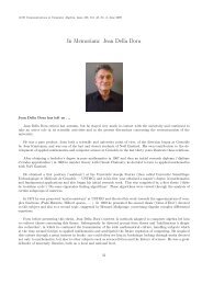
Philippe Flajolet, the Father of Analytic Combinatorics
Communicted by
Bruno Salvy, Bob Sedgewick, Michele Soria, Wojciech Szpankowski, Brigitte Vallee
Philippe Flajolet, mathematician and computer scientist extraordinaire, suddenly passed away on
March 22, 2011, at the prime of his career. He is celebrated for opening new lines of research in analysis of
algorithms, developing powerful new methods, and solving difficult open problems. His research contributions
will have impact for generations, and his approach to research, based on curiosity, a discriminating
taste, broad knowledge and interest, intellectual integrity, and a genuine sense of camaraderie, will serve
as an inspiration to those who knew him for years to come.
The common theme of Flajolet’s extensive and far-reaching body of work is the scientific approach to
the study of algorithms, including the development of requisite mathematical and computational tools.
During his forty years of research, he contributed nearly 200 publications, with an important proportion of
fundamental contributions and representing uncommon breadth and depth. He is best known for fundamental
advances in mathematical methods for the analysis of algorithms, and his research also opened new
avenues in various domains of applied computer science, including streaming algorithms, communication
protocols, database access methods, data mining, symbolic manipulation, text-processing algorithms, and
random generation. He exulted in sharing his passion: his papers had more than than a hundred different
co-authors and he was a regular presence at scientific meetings all over the world.
His research laid the foundation of a subfield of mathematics, now known as analytic combinatorics. His
lifework Analytic Combinatorics (Cambridge University Press, 2009, co-authored with R. Sedgewick) is
a prodigious achievement that now defines the field and is already recognized as an authoritative reference.
Analytic combinatorics is a modern basis for the quantitative study of combinatorial structures (such
as words, trees, mappings, and graphs), with applications to probabilistic study of algorithms that are
based on these structures. It also strongly influences other scientific domains, such as statistical physics,
computational biology, and information theory. With deep historic roots in classical analysis, the basis of
the field lies in the work of Knuth, who put the study of algorithms on a firm scientific basis starting in the
late 1960s with his classic series of books. Flajolet’s work takes the field forward by introducing original
approaches in combinatorics based on two types of methods: symbolic and analytic. The symbolic side is
90

Philippe Flajolet
based on the automation of decision procedures in combinatorial enumeration to derive characterizations of
generating functions. The analytic side treats those functions as functions in the complex plane and leads
to precise characterization of limit distributions. In the last few years, Flajolet was further extending and
generalizing this theory into a meeting point between information theory, probability theory and dynamical
systems.
Philippe Flajolet was born in Lyon on December 1, 1948. He graduated from Ecole Polytechnique in
Paris in 1970, and was immediately recruited as a junior researcher at the Institut National de Recherche
en Informatique et en Automatique (INRIA), where he spent his career. Attracted by linguistics and
logic, he worked on formal languages and computability with Maurice Nivat, obtaining a PhD from the
University of Paris 7 in 1973. Then, following Jean Vuillemin in the footsteps of Don Knuth, he turned
to the emerging field of analysis of algorithms and got a Doctorate in Sciences, both in mathematics and
computer science, from the University of Paris at Orsay in 1979. At INRIA, he created and led the ALGO
research group, which attracted visiting researchers from all over the world.
He held numerous visiting positions, at Waterloo, Stanford, Princeton, Wien, Barcelona, IBM and
the Bell Laboratories. He received several prizes, including the Grand Science Prize of UAP (1986), the
Computer Science Prize of the French Academy of Sciences (1994), and the Silver Medal of CNRS (2004).
He was elected a Corresponding Member (Junior Fellow) of the French Academy of Sciences in 1994, a
Member of the Academia Europaea in 1995, and a Member (Fellow) of the French Academy of Sciences in
2003.
A brilliant, insightful “honnête homme” with broad scientific interests, Philippe pursued new discoveries
in computer science and mathematics and shared them with students and colleagues for over 40 years with
enthusiasm, joy, generosity, and warmth. In France, he was the major reference at the interface between
mathematics and computer science and founded the “Alea” meetings that bring together combinatorialists,
probabilists and physicists to share problems and methods involving discrete randomness. More broadly,
he was the leading figure in the development of the international “AofA” community that is devoted
to research on probabilistic, combinatorial, and asymptotic methods in the analysis of algorithms. The
colleagues and students who are devoted to carrying on his work form the core of his primary legacy.
91

ACM Communications in Computer Algebra, Issue 176, Vol. 45, No. 2, June 2011
Abstracts of WWCA 2011 in Honor of Herb Wilf’s 80th Birthday
Communicated by Ilias Kotsireas and Eugene Zima
Author: Gert Almkvist
Affiliation: University of Lund, Sweden
Title: Ramanujan-like formulas for 1 and String Theory
π 2
Abstract: This is joint work with Jesus Guillera, Zaragoza. Using the Gromov-Witten potential from String
Theory we design a Maple programme to find formulas for 1 . One result is the new formula
π2 1
π 2 = 32
3
∞∑ (6n)!
n! 6 (532n2 + 126n + 9)
n=0
which can be used to compute an arbitrary decimal digit of
1
1000 2n+1
1
without computing the earlier digits.
π2 Author: George E. Andrews
Affiliation: Pennsylvania State University, USA
Title: Partition Function Differences, and Anti-Telescoping
Abstract: For decades partition function differences have been studied. These include a famous problem
of Henry Alder posed in the 1950’s and solved only recently by Yee, Oliver et al.. In 1978, Szekeres and
Richmond partially solved a problem of this type concerning the Rogers-Ramanujan continued fraction.
Unknown to them, the problem had essentially been solved by Ramanujan in the Lost Notebook. In this
talk, I will begin with the history of such problems. I will conclude with some observations on a method,
Anti-Telescoping, for treating some such problems. Here is a typical example of the questions posed.
The late Leon Ehrenpreis asked in 1987 if one could prove that the number of partitions of n into parts
congruent to 1 or 4 mod 5 is always at least as large as the number with parts congruent to 2 or 3 mod 5
WITHOUT using the Rogers-Ramanujan identities. Subsequently Baxter and I gave a ”sort of” solution to
the problem, and Kevin Kadell gave a complete solution in 1999. We shall describe how Anti-Telescoping
treats this problem.
Author: Miklos Bona
Affiliation: University of Florida, USA
Title: Permutations as Genome Rearrangements
Abstract: Given a permutation written in the one-line notation, such as 3147526, it is natural to ask how
many block transpositions (interchanges of two adjacent substrings) are needed to turn this permutation
into the increasing one. This has turned out to be a surprisingly difficult problem, and a long-standing
conjecture has recently been disproved in this area. If, on the other hand, we are allowed to interchange any
two blocks, then the best sorting algorithm is known. The average number of necessary block interchanges
has recently been computed, using some very unexpected tools from remote-looking areas of mathematics.
In this talk, we will review the results and open problems of these two families of questions, and suggest
92

WWCA 2011 Abstracts
another interesting open problem connected to them. We will say a few words about the biological motivation
of these questions, and discuss some of their variations as well. No previous knowledge of sorting
algorithms is necessary, and the talk will be accessible to students.
Authors: Rodney Canfield
Affiliation: University of Georgia, USA
Title: The Asymptotic Hadamard Conjecture
Abstract: The Hadamard Conjecture states that for every integer n which is divisable by 4 there is an
n × n matrix over {±1} whose rows are pairwise orthogonal. The first value of n in question is 668. Let
H nt equal the number of n × t matrices over {±1} whose rows are pairwise orthogonal. The Asymptotic
Hadamard Conjecture gives an asymptotic formula for H nt . The conjecture has been proven by de Launey
and Levin (2010) for t > n 12+ɛ . We are attempting to extend the range of validity for the formula.
Author: Sylvie Corteel
Affiliation: Universite Paris 7, France
Title: Enumeration of Staircase Tableaux
Abstract: Staircase tableaux were recently introduced by Williams and the speaker to capture the combinatorics
of the Partially Asymmetric Self Exclusion Process and the moments of the Askey Wilson
polynomials. In this talk the speaker will focus on the enumeration of staircase tableaux at various specializations
of the parameterizations; for example, we will see how to obtain the Catalan numbers, Fibonacci
numbers, Eulerian numbers, the number of permutations, and the number of matchings.
Author: Aviezri S. Fraenkel
Affiliation: Weizmann Institute of Science, Israel
Title: What’s a question to Herb Wilf’s answer?
Abstract: An answer doesn’t determine the matching question uniquely. Recently, Herb Wilf and Warren
Ewens wrote their revolutionary “There’s plenty of time for evolution”, in which they refuted the refutation
of Darwin’s theory that exponential time is needed for evolution. They argue that evolution progresses in
parallel, not in series, thereby reducing evolution time drastically. While reading this interesting treatise,
I asked myself what other theories (population genetics, phylogenetics, evolutionary biology, geology, geosciences
paleobiology, . . . ), could be consistent with their theory. I think that I was led to this question
since I recently became interested in “inverse problems” in the area of combinatorial games. Roughly
speaking, given a winning strategy, what’s a game that has the given winning strategy? I compounded
this with another question. The winning strategy of Wythoff type games on two piles of tokens is usually
given in the form of two complementary sequences of integers. What happens if the sequences are not
complementary? We give some questions to these answers.
Author: Ira Gessel
Affiliation: Brandeis University, USA
Title: On the WZ Method
Abstract: It is well known that the WZ method of Wilf and Zeilberger gives an efficient way of proving
hypergeometric series identities, but each example of the method is usually presented as an isolated application.
I will explain how nearly all examples of the WZ method may be associated with special cases of
the classical hypergeometric summation formulas of Gauss, Pfaff-Saalschutz, and Dougall.
93

Kotsireas
Author: Ian Goulden
Affiliation: University of Waterloo, Canada
Title: Combinatorics and the KP hierarchy
Abstract: Maps in an orientable surface of arbitrary genus and branched covers of the sphere can both
be represented by factorizations in the symmetric group, in which the subgroup generated by the factors
acts transitively on the underlying symbols (these are called ”transitive factorizations”). The generating
series for a large class of transitive factorizations satisfies the KP hierarchy. We shall discuss the KP
hierarchy and a new algebraic combinatorial proof of the fundamental result that relates Schur function
expansions of a series and the Plucker relations. As an application, we give a recurrence for triangulations
of a surface of arbitrary genus obtained from the simplest partial differential equation in the KP hierarchy.
The recurrence is very simple, and we do not know a combinatorial interpretation of it, yet it leads to
precise asymptotics for the number of triangulations with n edges, in a surface of genus g.
Author: Ronald Graham
Affiliation: UCSD, USA
Title: Joint statistics for permutations in S n and Eulerian numbers
Abstract: In this talk I will describe some recent results concerning the connection between the bubblesort
sorting algorithm and certain integer sequences used to analyze patterns that arise in juggling. The analysis
leads to new results on the joint distribution of the descent and maximum drop statistics of a permutation,
as well as a new class of identities for the classical Eulerian numbers.
Author: Andrew Granville
Affiliation: Université de Montreal, Canada
Title: More combinatorics and less analysis: A different approach to prime numbers
Abstract: Since Riemann’s memoir 150 years ago, the main approach to studying the distribution of prime
numbers has come from the study of the complex zeros of the analytic continuation of the Riemann zeta
function. Indeed many regard the study of the seeming combinatorial problem of counting primes as
tautologically the same as the study of zeta(s), as seems to be indicated by Riemann’s brilliant explicit
formula. In this talk we introduce the ”pretentious approach” of Soundararajan and the speaker to the
distribution of prime numbers, which is quite analogous to key ideas in additive combinatorics/number
theory and does not rest on the study of analytic continuations.
Author: Curtis Greene
Affiliation: Haverford College, USA
Title: Some Posets Related to Muirhead’s, Maclaurin’s, and Newton’s Inequalities
Abstract: Many classical inequalities such as those in title can be extended to familiar combinatorial
symmetric function families such as the elementary, homogeneous, power sum, and Schur polynomials. All
known instances of these extended inequalities hold in a strong form (”Y-positivity”), and these results
are apparently new. Our analysis has involved certain posets which are of some interest in their own
right, including the ”double-majorization order” on partitions and the lattice of 2-rowed standard Young
tableaux. We will survey some of these techniques, and report on some recent results and open problems.
This is joint work with Mark Skandera and Jonathan Lima.
94

WWCA 2011 Abstracts
Author: Joan Hutchison
Affiliation: Macalester College, USA
Title: Some Challenges in List-Colouring Planar Graphs
Abstract: A graph G is said to be L-list-colorable when each vertex v is assigned a list L(v) of colors and
G can be properly colored so that each v receives a color from L(v). Typically the lists L may vary from
vertex to vertex. A graph is said to be k-list-colorable when it can be L-list-colored whenever every list
L(v) contains at least k colors. A celebrated theorem of C. Thomassen proves that every planar graph can
be 5-list-colored. An unresolved question of M.O. Albertson asks whether there is a distance d > 0 such
that whenever a set P of vertices of a planar graph G are precolored and are mutually at distance at least
d from one another, the precoloring extends to a 5-list-coloring of G. In this talk we give some partial
affirmative answers to Albertson’s question and investigate the extent to which Thomassen’s theorem and
Albertson’s question are best possible. This talk includes joint work with co-authors M.O. Albertson, M.
Axenovich, and M.A. Lastrina.
Author: David M.R. Jackson
Affiliation: University of Waterloo, Canada
Title: Enumerative Aspects of Cactus Graphs
Abstract: I shall discuss enumerative aspects of cactus graphs in the context of a formal analogue of the
Legendre transform. Extensions to the m-th order Legendre transform will be considered, as well as the
impact of this work on other areas. Attention will be confined to the univariate case, although extension
to the multivariate case seems feasible.
Author: Christian Krattenthaler
Affiliation: University of Vienna, Austria
Title: Cyclic Sieving for Generalised Non-Crossing Partitions Associated to Complex Reflection Groups
Abstract: Cyclic sieving is a(n enumerative) phenomenon formulated by Reiner, Stanton and White. Bessis
and Reiner proposed two conjectures on cyclic sieving phenomena for the generalised non-crossing partitions
associated to complex reflection groups of Armstrong and Bessis. I shall first explain what cyclic sieving
and these generalised non-crossing partitions are about, and then report the main ideas of a proof of the
above two conjectures. Part of this work is in collaboration with Thomas Muller.
Author: Victor H. Moll
Affiliation: Tulane University, USA
Title: p-adic Valuations of Sequences: Examples in Search of a Theory
Abstract: In this lecture we present a variety of results and problems related to the p-adic valuation of
classical sequences. Examples include Stirling numbers and the ASM-numbers that count the number of
alternating sign matrices. An attempt to form a general theory will be discussed.
Author: Andrew Odlyzko
Affiliation: University of Minnesota, USA
Title: Primes, Graphs and Generating Functions
Abstract: Herb Wilf had extensive influence on the development of many fields of mathematics, both
through his own research, and through asking penetrating questions. Some personal reminiscences of his
influence and his collaborations will be presented.
95

Kotsireas
Author: Peter Paule
Affiliation: Research Institute for Symbolic Computation, Johannes Kepler University Linz, Austria
Title: Proving strategies of WZ-type for modular forms
Abstract: In the context of WZ-theory Lily Yen and others have shown how hypergeometric identities can be
proven by checking finitely many cases only. The talk, being joint work with Silviu Radu (RISC), discusses
the algorithmic application of similar ideas, including the role of recurrences, to problems involving modular
forms. One of the illustrating examples is a new proof of Ramanujan’s celebrated partition congruences
for powers of 11.
Author: Robin Pemantle
Affiliation: University of Pennsylvania, USA
Title: Zeros of Complex Polynomials and their Derivatives
Abstract: The zeros of f ′ are known to lie in the convex hull of the zeros of f. Often one can say much
more. When the zeros of f are independent random picks from a distribution, it turns out that the zeros
of f ′ have the same distribution in the limit. Under further assumptions, nearly all of the zeros of f ′ are
matched to corresponding zeros of f. This is joint work with I. Rivin.
Author: Marko Petkovsek
Affiliation: University of Ljubljana, Slovenia
Title: On Enumeration of Structures with no Forbidden Substructures
Abstract: Many interesting classes of combinatorial structures are defined by restricting some general class
of structures to those structures that avoid certain “forbidden” substructures. Examples include words
avoiding forbidden subwords or subsequences, permutations avoiding forbidden patterns, matrices avoiding
forbidden submatrices, graphs avoiding forbidden subgraphs, induced subgraphs, minors, or topological
minors. We will try to look at the abundance of enumeration problems (solved and unsolved) presented
by such classes.
Authors: Bruce E. Sagan
Affiliation: Michigan State University, USA
Title: Mahonian Pairs
Abstract: We introduce the notion of a Mahonian pair. Consider the set, P ∗ , of all words having the
positive integers as alphabet. Given finite subsets S, T ⊂ P ∗ , we say that (S, T ) is a Mahonian pair if the
distribution of the major index, maj, over S is the same as the distribution of the inversion number, inv,
over T . So the well-known fact that maj and inv are equidistributed over the symmetric group, S n , can
be expressed by saying that (S n , S n ) is a Mahonian pair. We investigate various Mahonian pairs (S, T )
with S ≠ T . Our principal tool is Foata’s fundamental bijection φ : P ∗ → P ∗ since it has the property
that maj w = inv φ(w) for any word w. We consider various families of words associate with Catalan and
Fibonacci numbers. Various other ideas come into play such as the ranks and Durfee square size of integer
partitions, the Catalan triangle, and various q-analogues.
Author: Carla D. Savage
Affiliation: NCSU, USA
96

WWCA 2011 Abstracts
Title: Generalized Lecture Hall Partitions and Eulerian Polynomials
Abstract: Lecture hall partitions, introduced by Bousquet-Melou and Eriksson in 1997, are nonnegative
integer sequences (x 1 , x 2 , ..., x n ) satisfying x i /i

Kotsireas
groups W = S n for n ≤ 10 they are (modulo a few mild technical hypotheses) the only examples.
Author: Volker Strehl
Affiliation: Universitaet Erlangen, Germany
Title: Aspects of a Combinatorial Annihilation Process
Abstract: The asymmetric annihilation process has been introduced by A. Ayyer and K. Mallick (J Phys
A, 2010) and has been further studied by A. Ayyer and the author (FPSAC 2010). It is similar in spirit to
the familiar TASEP model, but it also allows for the annihilation of neighbouring particles. In this talk I
will describe an algebraic framework for a fully parametrized version of the annihilation process, including
the derivation of its partition function.
Author: Michelle Wachs
Affiliation: University of Miami, USA
Title: Unimodality of q-Eulerian Numbers and p, q-Eulerian Numbers
Abstract: The Eulerian numbers enumerate permutations in the symmetric group S n by their number of
excedances or by their number of descents. It is well known that they form a symmetric and unimodal
sequence of integers. In this talk, which is based on work with John Shareshian and Anthony Henderson,
we consider the q-analog of the Eulerian numbers obtained from the joint distribution of the major index
and the excedance number, and the p, q-analog of the Eulerian numbers obtained by considering the joint
distribution of the major index, descent number and excedance number. We show that the q-Eulerian
numbers form a symmetric and unimodal sequence of polynomials in q and the p, q-Eulerian numbers
refined by cycle type form a symmetric and unimodal sequence of polynomials in p and q. The proofs of
these results rely on the Eulerian quasisymmetric functions introduced in joint work with Shareshian, on
symmetric and quasisymmetric function theory, and on representation theory of the symmetric group.
Author: Herbert S. Wilf
Affiliation: University of Pennsylvania, USA
Title: Two problems in combinatorial biology
Abstract: The talk concerns two problems that were studied by Warren Ewens and myself and published in
PNAS. The first concerns recognition of a disease epidemic as opposed to just a coincidental large number
of cases in a small geographical area. The second is about evolution. One objection that has been raised
to Darwinian evolution is that too much time would be required for the necessary numbers of random
mutations to happen, as needed to encode a complex organism. We show that if a simple model of the
way natural selection and evolution work together is studied, it shows that in a very short time, a simple
word can be transformed into a complex one with random transformations of the letters. So in fact there
is plenty of time for evolution.
Author: Doron Zeilberger
Affiliation: Rutgers University, USA
Title: Automatic Generation of Theorems and Proofs on Enumerating Consecutive WILF-classes
Abstract: Shalosh B. Ekhad can ANSWER (in WILF’s sense of the word) the question “how many permutations
avoid such and such (classical) pattern” for quite a few “such and such” (classical) patterns,
but, so far, and most probably never, for ALL patterns. But it sure can ANSWER (in W’s sense) the
analogous question for consecutive-WILF patterns, introduced by Sergi Elizalde and Marc Noy. Joint work
with Andrew Baxter, Brian Nakamura, and of course, Shalosh B. Ekhad.
98

WWCA 2011 Abstracts
Author: Eugene Zima
Affiliation: Wilfrid Laurier University, Canada
Title: Synthetic division in the context of indefinite summation
Abstract: A modification of an algorithm for indefinite rational summation is presented. It is based on direct
divisibility test in the ring of linear difference operators with polynomial coefficients. When the rational
function is not summable it provides solution to the additive decomposition problem with minimal degree
of the denominator of the rational part. The algorithm solves the problem in time which is polynomial in
the size of the input and linear in the minimal possible size of the output. This removes all non-essential
dependencies of the running time of the algorithm from the dispersion of the input. The result is extended
to the case of quasi-rational indefinite summation. Prototype implementation of the algorithm in Maple
together with succinct representation of the intermediate results is discussed.
99

ACM Communications in Computer Algebra, Issue 176, Vol. 45, No. 2, June 2011
East Coast Computer Algebra Day 2011 Abstracts
Communicated by John May
Invited Talks
Christopher Brown (US Naval Academy): Computing with semi-algebraic sets: from problem to solution
Abstract: In symbolic computing, most of us are familiar with the basics of computing with polynomial
systems over algebraically closed fields. We speak of systems of equations or, equivalently, the varieties they
define; of elimination or projection. Most of the community is much less familiar with polynomial systems
over the reals, where the fundamental questions and the kinds of solutions we get are very different. We
speak of Tarski formulas and semi-algebraic sets, and problems from formal logic like quantifier elimination.
This talk first looks at why the basic problem is different in the real case, and what solutions look like in
the real case. It then looks at several algorithms, both recent and not so recent, that seem to be answering
the same questions, and tries to understand them by their different perspectives of what the problem is
and what constitutes a solution.
Clément Pernet (Unversité Joseph Fourier): Eliminations and echelon forms in exact linear
Abstract: Gaussian elimination and the computation of the numerous related matrix factorizations are a
key component in the design of high performance mathematical computation software. This talk is about a
collection of algorithmic and implementation techniques that we found of prime importance when dealing
with these computations in computer algebra. After setting algorithmic relations between most common
gaussian elimination based matrix factorizations and normal forms, we will propose a set of reductions of
all these computations to a universal matrix factorization, justified by time and space complexity analysis.
We will then approach some aspects of dedicated implementations over GF(2) and the parallelization of
gaussian elimination, showing in particular advantages over numerical linear algebra.
Victoria Powers (Emory University): Rational certificates of positivity
Abstract: Let R[X] denote the real polynomial ring in n variables R[X 1 , . . . , X n ]. Given f in R[X] and
suppose f > 0 or f ≥ 0 on a semialgebraic set K ⊆ R n , i.e., one defined by a finite number of polynomial
inequalities. By a “certificate of positivity” for f on K, we mean an expression for f, usually involving
sums of squares and the defining polynomials of K, from which one can observe the positivity condition
immediately. In recent years, techniques from semidefinite programming have produced algorithms for
finding certificates of positivity; these algorithms have many applications in optimization, control theory,
and other areas. However, the output of these algorithms is, in general, numerical, while for many applications
exact polynomial identities are needed. In this talk, we look at questions such as these: If f
and K are defined over Q, does there exist a certificate of positivity for f on K for which the sums of
squares are sums of squares of polynomials defined over Q? How can a numerical certificate of positivity
be transformed into an exact rational identity? We will discuss theoretical results as well as hybrid
symbolic-numeric algorithms due to Peyrl-Parrilo, Kaltofen-Li-Yang-Zhi, and others.
100

ECCAD 2011 Abstracts
Software Demonstration
Authors: Changbo Chen (University of Western Ontario), James H. Davenport (University of Bath),
François Lemaire (Université de Lille 1), Marc Moreno Maza (University of Western Ontario), Bican
Xia (Peking University), Rong Xiao (University of Western Ontario), Yuzhen Xie (University of Western
Ontario)
Title: Computing the real solutions of polynomial systems with the RegularChains library in Maple
Abstract: Computing and manipulating the real solutions of polynomial systems is a requirement for many
application areas such as biological modeling, robotics, program verification, to name a few.
The RegularChains library in Maple provides a collection of tools for dealing with systems of polynomial
equations, inequations and inequalities. These tools include isolating/counting the real solutions of zerodimensional
systems, describing real solutions of positive dimensional systems, classifying the number of
real roots of parametric systems, finding sample points (thus determining emptiness) of semi-algebraic
sets, performing set theoretical operations on semi-algebraic sets as well as computing cylindrical algebraic
decompositions.
The software demonstration would be articulated around four problems taken respectively in the following
application areas: branch cut computations, verification of real solvers, realization of matroids, equilibria
of biological systems.
Posters
Authors: R.F. Burger (University of Waterloo), G. Labahn (University of Waterloo)
Title: Closed form solutions of linear differential equations having elliptic function coefficients.
Abstract: We consider the problem of finding closed form solutions of linear homogeneous ordinary differential
equations having coefficients which are elliptic functions. A complete algorithm is presented, applicable
to differential equations of any order, which finds all hyperexponential solutions of the form exp( ∫ x r(u)du),
where r(x) ∈ C(℘(x), ℘ ′ (x)). For differential equations of order higher than two, the method has been
found to be more practical than other known methods.
Authors: Rob M. Corless (University of Western Ontario), Gema Díaz Toca (Universidad de Murcia), Mario
Fioravanti (Universidad de Cantabria), Laureano Gonzalez-Vega (Universidad de Cantabria), Ignacio F.
Rúa (Universidad de Oviedo), Azar Shakoori (Universidad de Cantabria)
Title: Computing the topology of an implicit or a parametric plane curve whose defining equations can
only be evaluated.
Abstract: The problem of computing the topological graph of an implicitly defined algebraic plane curve
has received special attention from the CAGD and Symbolic Computation communities, independently. In
CAGD, having a robust, accurate and efficient algorithm to find the graph is a key tool in solving many
important problems. For the Symbolic Computation community, on the other hand, such a problem has
been the motivation for many achievements in the study of subresultants, symbolic real root counting,
infinitesimal computations, etc. In many practical problems, one is interested in computing the topology
of an algebraic curve whose parametric or implicit equations have rather high degrees, numerous terms
and very large coefficients. Applying the currently available methods for computing the topology of the
curve, with such polynomial equations, requires a big amount of memory space and a significant amount
of computing time. This is one of the main reasons why, in this work, we assume that neither the implicit
equation nor the parametrization of the given curve is known. Instead, sufficient number of points in the
curve and the corresponding values of the equations and derivatives are known, and the degree is also
given or can be deduced. The method presented here allows the computation of the topology of the curve
101

May
using only this data, and it is based on the “polynomial algebra by values” methodology which has been
presented in our previous works.
Author: Somit Gupta (University of Waterloo)
Title: Division of Polynomial Matrices.
Abstract: For any N ∈ K[x] n×n and a non singular D ∈ K[x] n×n , there are unique Q, R ∈ K[x] n×n , such
that N = QD + R and RD −1 is strictly proper. We present an approach, that given N ∈ K[x] n×n and a
non singular column reduced D ∈ K[x] n×n , we can reduce the problem of division of N by D to a single
polynomial matrix inversion, multiplication and subtraction, over the ring K[x]/(x t ),where t is bounded by
the degree of D + degree of N. Our approach can be considered as a generalization of the newton iteration
method for division of polynomials over K[x]. We also discuss some alternative approaches.
Author: Tom Robinson (University of Waterloo)
Title: Effective Support of Learning with a Computer Algebra System.
Abstract: Computer Algebra Systems (CAS) have long been used in education. As with any educational
software, the goals of using a CAS include improving how quickly and easily a student can learn, as well
as increasing his or her depth of understanding.
Instructional material that teaches a student to use a CAS while at the same time introducing the student to
new mathematical concepts can impose a high cognitive load and leave the student with little understanding
of either the CAS or the mathematics.
In this poster I will present a framework describing how students learn and how good instructional design
can better support that learning through control of cognitive load. I will also present the results from a
number of studies.
Authors: Mark Giesbrecht and Daniel S. Roche (University of Waterloo)
Title: Faster Sparse Interpolation over Finite Fields and Complex Numbers.
Abstract: The problem of interpolating an unknown sparse polynomial from a black box for evaluations is
considered, when the coefficients come from a large finite field or are approximations to complex numbers.
We present a new randomization and prove that it makes all coefficients distinct, or in the approximate
case, sufficiently far apart, with high probability. This allows us to improve on the recent algorithm of
Garg and Schost (TCS 2009) by uniquely identifying terms in modular evaluations by the coefficients,
thus avoiding the need for root finding over Z[x]. Over large, unchosen finite fields, our probabilistic
algorithm improves the complexity by a factor of t, the number of terms in the unknown polynomial.
Over approximate complex numbers, we prove that the algorithm is provably numerically stable, and the
required precision is polynomially bounded by the number of terms and the logarithm of degree of the
unknown polynomial. Other approximate sparse interpolation algorithms are not known to be numerically
stable, although they require fewer black box evaluations than ours. We implemented these algorithms in
C++ and demonstrate that their experimental performance confirms our theoretical results.
Authors: Weidong Liao and Osman Guzide (Shepherd University)
Title: High Performance GCD Computation with GPUs.
Abstract: The Greatest Common Divisor (GCD) computation is one of the meta-services used by many
mathematical computations. If a separate dedicated and efficient service can be provided, various research
efforts which require GCD computation can have their focus elsewhere.
In this poster we describe our result of comparative study of several approaches to utilizing GPU computing
to accelerate GCD computation. Implementation of a variety of GCD algorithms (such as the Euclidean
Algorithm and the Binary GCD Algorithm) has also been compared. Since CUDA is so far one of the
most popular APIs for GPU computing, our experiments are mostly based on CUDA APIs, including the
102

ECCAD 2011 Abstracts
original CUDA API and one of its Java wrappers, JCUDA. The comparison is done on the aspects of
simplicity and efficiency.
Authors: David Augenblick, Mark Boady, Bruce Char, Jeremy Johnson, and LC Meng (all Drexel University)
Title: Individualized Assignments and Assessment through Automated Grading.
Abstract: We have used an on-line automatic grading system, Maple TA, in a course on technical computing
with over 900 freshman engineering students. Students spend ten hours per term in labs with face-to-face
contact with instructional staff. On-line pre-lab quizzes guide student lab preparation. Post-lab on-line
assignments provide further practice, solidifying skills. Symbolic computation generates a unique autogradable
version of the problem sets for each student. Allowing multiple attempts per quiz encourages
students to continue work until they know they have solved the problem. Peer-led and staff tutoring
(face-to-face and on-line) provides “just in time” help for post-lab quizzes.
On-line storage of all test results facilitates the collection of statistics on all regularly graded materials.
These can be used to identify class-wide and individual strengths and weaknesses, as well as longitudinal
information on learning patterns and retention.
IT expertise is needed to keep services running with high availability and reliability. Software engineering
discipline is needed to construct robust questions and grading procedures. Current limitations of autograding
technology present pedagogical challenges.
What began as a necessity has become an essential learning tool, providing students with a learning tool
that has 24/7 availability, gives immediate feedback, and is scalable.
Authors: Oleg Golubitsky (Google, Inc.), Vadim Mazalov (University of Western Ontario), Stephen M.
Watt (University of Western Ontario)
Title: Integral Invariants in Recognition of Handwritten Symbols.
Abstract: It was shown in previous work that truncated Legendre-Sobolev expansions of coordinate functions
of stroke curves can be applied to recognition of handwritten mathematical symbols. Test results
confirm that this technique is indeed effective and allows to achieve 97.5% recognition rate. In this work, we
allow the symbols to be subject to a rotation which commonly occurs in practice. We ask to which extent
these transformations affect the classification rates and present a new algorithm for classifying symbols in
the presence of such transformations, based on the theory of integral invariants of parametric curves. The
proposed algorithm is on-line, in the sense that most computation is done while the symbol is written, and
therefore does not cause delays.
Authors: Marc Moreno Maza and Paul Vrbik (University of Western Ontario)
Title: Inverting Matrices Modulo Regular Chains
Abstract: Given any set of polynomials (in several variables), F, it is natural to investigate the set of points
for which the polynomials vanish simultaneously (the so-called variety of F). When F is composed of linear
systems we do Gaussian elimination which, by producing an equivalent upper triangular system, allows
one to solve for each unknown by back substitution. Gaussian elimination can be extended to non-linear
systems (Buchberger’s algorithm) but the “triangular” objects obtained this way do not necessary allow
for non-trivial back substitution.
This is the motivation behind the theory (and technology) of “regular chains”. Here we can generate a
regular chain that encodes each “component” of the solution set. These encodings ensure (among other
things) the “well behaved” back substitution we require to obtain the zeros of the original system.
In practice, regular chains that have an equal number of equations and unknowns (i.e. zero dimensional
systems) are of great interest. In this study, we consider solving ”parametric” linear systems where the
parameters are constrained by such regular chains.
103

May
Specifically, we adapt the Leverrier-Faddeev algorithm for matrix inversion (which requires only a single
division) to avoid many costly regular chain inversions. Although this algorithm has worse computational
complexity than the extended GCD approach, it can solve a wider range of problems than the current
(naive) implementation.
We present experimental and theoretical results, as well as some conjectures about positive dimensional
cases.
Authors: Scott MacLean, George Labahn, Edward Lank, Mirette Marzouk, and David Tausky (all University
of Waterloo)
Title: MathBrush: A pen-based interactive math system for Tablet PC and iPad.
Abstract: Traditional methods of working with mathematics on computers, such as LaTeX, Maple, and
Mathematica, can be error-prone and difficult to learn. We aim to provide via MathBrush a more intuitive
environment for inputting and manipulating mathematical expressions. Using MathBrush, the user draws
an expression as (s)he would using pen and paper. The system recognizes the mathematical semantics
of the drawing and inserts the expression into a worksheet, after which the user may manipulate it using
computer algebra system commands invoked through a context-sensitive pen-based interface. We provide
a general overview of the MathBrush system, including current status and future directions.
Authors: Bryan Youse, B. David Saunders, and David Harlan Wood (all University of Delaware)
Title: Numeric-Symbolic Exact Rational Linear System Solver.
Abstract: An iterative refinement approach is taken to rational linear system solving. Such methods produce,
for each entry of the solution vector, a rational approximation with denominator a power of 2. From
this the correct rational entry can be reconstructed. Our iteration is a numeric-symbolic hybrid in that
it uses an approximate numeric solver at each step together with a symbolic (exact arithmetic) residual
computation and symbolic rational reconstruction. The rational solution may be checked symbolically (exactly).
However, there is some possibility of failure of convergence, usually due to numeric ill-conditioning.
We present our implementation details and show experimental data.
Authors: G.A. Kalugin, R.M. Corless, and D.J. Jeffrey (all University of Western Ontario)
Title: Padé approximants and a Stieltjes integral for the Lambert W function
Abstract: The Lambert W function is defined to be the multivalued inverse of the function W ↦→ W e W , i.e.
it satisfies the equation z = W (z)e W (z) . The function has many applications in various areas of science,
engineering and education, particularly, in computer algebra systems. In this work it is established that
W (z)/z is a Stieltjes function. This fact has many interesting consequences. One of them is applicability of
a well-developed theory of Padé approximants to Stieltjes series, which proves the existence and convergence
of Padé approximants for function W (z)/z. This is used to compute values of W in symbolic computations.
In the work there are presented examples using Maple.
Authors: Fatima K. Abu Salem (American University of Beirut)
Title: Parallel and Cache-efficient Hensel Lifting.
Abstract: We present work in progress towards a high performance (HP) design for Hensel lifting in the case
of bivariate polynomials over a finite field F q . We discuss techniques that improve on data locality, which
in turn is becoming increasingly important in today’s algorithm design. We also discuss how to re-organise
the iterative computations involved in the process into a sequence of rounds each of which can be executed
in parallel. Let f ∈ F q [x, y], and write n = deg(f). We wish to obtain a polynomial factorisation of f into
two factors g and h. Write f = ∑ n
k=0 f ky k where f k ∈ F q [x] and deg(f k ) = n − k. Suppose we were given
a (boundary) factorisation of the form f 0 = g 0 h 0 , where g 0 and h 0 belong to F q [x]. We wish to ‘lift’ this
boundary factorisation into a full polynomial factorisation of f in F q [x, y]. Under certain conditions, the
104

ECCAD 2011 Abstracts
following lifting equation helps produce all monic factors of f with total degree between 1 and ⌊n/2⌋:
(
) (
)
∑k−1
∑k−1
g k ≡ v f k − g i h k−i mod g 0 , h k ≡ u f k − g i h k−i mod h 0
i=1
At the level of concurrency, we show that the sequential order of computations which stipulates that in
the kth iteration a polynomial g k (or h k ) can only be computed after g k−1 and h k−1 have been obtained,
can be overcome by a sequence of parallel rounds such that in round k ′ all of the following polynomial
products can be obtained: {g i h j } such that (i, j) ∈ {1, . . . , k ′ } 2 ∧ (i = k ′ ∨ j = k ′ ). As a consequence
of this parallelisation one can start producing g k (or h k ) whenever g ⌈k/2⌉ and h ⌈k/2⌉ have been obtained,
and it can be shown that the number of rounds grows asymptotically alike to the total number of lifting
steps required to terminate. To address data locality, we associate the order of polynomial computations
g i h j occuring in a given parallel round k ′ with the address pair (i, j). We propose a traversal of the twodimensional
grid in the following order: In a given parallel round k ′ we first produce g k ′h k ′ and then, after
any g i h k ′ we enlist g i−1 h k ′ if i > 1; otherwise, we enlist g k ′h j−1 . Such a traversal improves on temporal
locality as well as data locality, specifically so as this traversal incurs exactly one jump in the address space
that is of stride asymptotically greater than one. Last, we incorporate the heap data structure to merge
(
terms arising in polynomial products to compute g k = v
f k − ∑ k−1
i=1
i=1
∑ #gi
s=1 g i,sh k−i
)
where #g i denotes the
number of nonzero terms of g i and g i,s denotes the sth nonzero term of g i (similarly for h k ). As observed
in the successful results of (Monagan and Pearce 2007-08-09-10), heap based computations defined as such
reduce the auxiliary space wasted on intermediary results and in this context would have sizes that fit in
cache, given reasonably sparse polynomials.
Authors: Thomas Wolf (Brock University), Eberhard Schruefer (Frauenhofer Institute)
Title: A solver for large sparse linear algebraic systems.
Abstract: The study of integrability of non-abelian Laurent ODEs includes the computation of symmetries,
first integrals and Lax-pairs. Using the method of undetermined coefficients the computational tasks include
the solution of polynomial algebraic systems that are either non-linear and involve a few hundred variables
or that are linear but very large. A specialized solver for large sparse and overdetermined linear systems
has been developed that was able to determine the general solution of systems with over a billion equations
for 170 million variables.
Authors: Marc Moreno Maza (University of Western Ontario), Wei Pan (Intel Corporation)
Title: Solving Bivariate Polynomial Systems on a GPU.
Abstract: We present a CUDA implementation of dense multivariate polynomial arithmetic based on
Fast Fourier Transforms (FFT) over finite fields. Our core routine computes on the device (GPU) the
subresultant chain of two multivariate polynomials with respect to a given variable. This subresultant chain
is encoded by values on a FFT grid and is manipulated from the host (CPU) in higher-level procedures,
for instance for polynomial GCDs modulo regular chains.
We have realized a bivariate polynomial system solver supported by our GPU code. Our experimental
results (including detailed profiling information and benchmarks against a serial polynomial system solver
implementing the same algorithm) demonstrate that our strategy is well suited for GPU implementation
and provides large speedup factors with respect to pure CPU code.
Authors: George Labahn (University of Waterloo), Jason Peasgood (University of Waterloo), Bruno Salvy
(INRIA Paris-Rocquencourt)
Title: Some Integrals Involving Holonomic Functions.
Abstract: We describe an algorithm that takes as input two holonomic functions, f and g given by differential
equations with polynomial coefficients along with some extra information, and outputs a differential
105

May
equation that is satisfied by ∫ ∞
0
f(t)g(xt)dt. The resulting differential equation also has polynomial coefficients
as well as possibly a non homogeous term that is computable.
Authors: Somit Gupta, Soumojit Sarkar, Arne Storjohann, and Johnny Valeriote (all University of Waterloo)
Title: Triangular x-basis decompositions and derandomization of linear algebra algorithms over K[x]
Abstract: Deterministic algorithms are proposed for some computational problems that take as input a
nonsingular polynomial matrix A over K[x], K an abstract field, including solving a linear system involving
A and computing a row reduced form of A. The fastest known algorithms for linear system solving based
on high-order lifting, and for row reduction based on fast minimal approximant basis computation , use
randomization to find either a linear or small degree polynomial that is relatively prime to det A. We
derandomize these algorithms by first computing a factorization of A = UH, with x not dividing det U
and x − 1 not dividing det H. A partial linearization technique, that is widely applicable also to other
problems, is developed to transform a system involving H, which may have some columns of large degrees,
to an equivalent system that has degrees reduced to that of the average column degree.
Authors: Curtis Bright and Arne Storjohann (University of Waterloo)
Title: Vector Rational Number Reconstruction
Abstract: The final step of some algebraic algorithms is to reconstruct the common denominator d of a
collection of rational numbers (n i /d) 1≤i≤n from their images (a i ) 1≤i≤n mod M, subject to a condition such
as 0 < d ≤ N and |n i | ≤ N for a given magnitude bound N. Applying elementwise rational number
reconstruction requires that M ∈ Ω(N 2 ). Using the gradual sublattice reduction algorithm of van Hoeij
and Novocin, we show how to perform the reconstruction efficiently even when the modulus satisfies a
considerably smaller magnitude bound M ∈ Ω(N 1+1/c ) for c a small constant, for example 2 ≤ c ≤ 5.
Assuming c ∈ O(1) the cost of the approach is O(n(log M) 3 ) bit operations using the original LLL lattice
reduction algorithm, but is reduced to O(n(log M) 2 ) bit operations by incorporating the L 2 variant of
Nguyen and Stehlé. As an application, we give a robust method for reconstructing the rational solution
vector of a linear system from its image, such as obtained by a solver using p-adic lifting.
106

ACM Communications in Computer Algebra, Vol. 45, No. 2, Issue 176, June 2011
ISSAC 2011 Poster Abstracts
Communicated by Manuel Kauers
Parallel and Cache-efficient Hensel Lifting
Fatima K. Abu Salem
Computer Science Department, American University of Beirut
P. O. Box 11-0236, Riad El Solh, Beirut 1107 2020, Lebanon
fatima.abusalem@aub.edu.lb
We present work in progress towards a high performance (HP) design for Hensel lifting bivariate polynomial
factorisation over a finite field F q . We discuss techniques that improve on data locality, which in
turn is becoming increasingly important in today’s algorithm design. We also discuss how to reorganise
the iterative computations involved in the process into a sequence of rounds each of which can be executed
in parallel. We propose the use of heaps, as inspired by successful results to perform polynomial multiplication
and division using the distributed polynomial representation (see Monagan and Pearce’s work
as in [1, 3, 3, 4], to name a few). Additionally, we associate the order of polynomial computations with
two-dimensional indices, and suggest a traversal of the two-dimensional grid in a manner that allows an
evaluation order of the dependency graph which improves upon locality.
Let f ∈ F q [x, y] where q is a prime power, and n = deg(f). We wish to obtain a polynomial factorisation
of f into two factors g and h such that f = gh. Write f = ∑ n
k=0 f ky k where f k ∈ F q [x] and deg(f k ) = n−k.
Suppose we were given a (boundary) factorisation of the form f 0 = g 0 h 0 , where f 0 is squarefree, and g 0
and h 0 belong to F q [x]. We wish to lift this boundary factorisation into a full polynomial factorisation of
f in F q [x, y]. Let d = gcd(g 0 , h 0 ) with u and v chosen such that ug 0 + vh 0 = d. When d = 1 and under
certain restrictions governing the degrees of each g k and h k , there will be at most one way of defining g k
and h k as follows: (
) (
)
∑k−1
∑k−1
g k ≡ v f k − g i h k−i mod g 0 , h k ≡ u f k − g i h k−i mod h 0 (1)
i=1
If the degree restrictions are observed one continues lifting; else, one halts lifting from the given pair
(g 0 , h 0 ). It can be shown that there exists a certain boundary factorisation by which one can produce all
monic factors of f with total degree between 1 and ⌊n/2⌋.
Computation in the order stipulated by Eq. 1 not only restricts parallelism to a very limited scale, it
also can be shown to produce bad memory performance. We show that the sequential order of computations
which stipulates that in the kth iteration a polynomial g k (or h k ) can only be computed after g k−1 and
h k−1 have been obtained, can be overcome by a sequence of parallel rounds such that in round k ′ all of the
following polynomial products can be obtained: {g i h j } such that (i, j) ∈ {1, . . . , k ′ } 2 ∧ (i = k ′ ∨ j = k ′ ).
Consequently, one can start producing g k (or h k ) whenever g ⌈k/2⌉ and h ⌈k/2⌉ have been obtained, and it
can be shown that the number of parallel rounds grows asymptotically alike to the total number of lifting
steps required to terminate. An extra component of concurrency can be further obtained, as partial terms
appearing in g k can kick-start computations contributing to {g ′ k } k ′ >k – similarly for h k . Such concurrency
reduces the number of synchronisation barriers needed as it allows processors to hop vertically across the
i=1
107

Vol. 45, No. 2, Issue 176, June 2011
ISSAC 2011 Posters
parallel rounds. We sketch a brief example here. Let f be given such that g 0 = x 8 + x 3 and h 0 = x 8 + 1.
After producing u and v, we get g 1 h 1 = p 1 1 + p1 2 where p1 1 = 2x14 + 3x 13 + 4x 12 + 4x 11 denotes the first
four terms of g 1 h 1 and p 1 2 = 3x8 + 2x 7 + x 6 + x 5 denotes the remaining four terms of g 1 h 1 . Each of
p 1 1 and p1 2 can be used to compute partial terms of g 2 such that g 2 = v(f 2 − p 1 1 ) mod g 0 − v(p 1 2 ) mod g 0.
This generates two batches of partial terms independently, denoted by p 2 1 = x5 + 4x 4 + x 3 + x and
p 2 2 = 3x6 +4x 5 +2x 4 +4x 3 for the first and second batches respectively, such that p 2 1 can start computations
on g 3 independently from p 2 2 . As such, we can start producing the first of the two parenthesised expressions
in g 3 = v(f 3 − g 1 h 2 − p 2 1 h 1) mod g 0 − v(p 2 2 h 1) mod g 0 whilst g 2 is still being computed.
To address data locality, we associate the order of polynomial computations g i h j occuring in a given
parallel round k ′ with the address pair (i, j). We propose a traversal of the two-dimensional grid in the
following order: In a given parallel round k ′ we first produce g k ′h k ′ and then, after any g i h k ′ we enlist
g i−1 h k ′ if i > 1; otherwise, we enlist g k ′h j−1 . For example, suppose that the g (and h) polynomials are
stored consecutively in the order by which they are being produced, and trace for instance, the execution
following the production of g 4 and h 4 . The parallel round ensuing proceeds as follows, where the right
arrow traces the order of execution: g 4 h 4 → g 3 h 4 → g 2 h 4 → g 1 h 4 → g 4 h 1 → g 4 h 2 → g 4 h 3 . We show that
this traversal improves on data locality, specifically that it incurs exactly one jump in the address space
that is of stride asymptotically greater than one (in this case, the jump from g 1 h 4 to g 4 h 1 ). This traversal
can also be automated leading to a cache-oblivious performance.
Consider the distributed polynomial representation, where a polynomial is represented as a sum of
terms sorted in a monomial ordering. Using this representation, we incorporate the binary heap data
structure to merge terms arising in the polynomial products. Let #g i denote the ( number of nonzero terms
of g i and g i,s denote the sth nonzero term of g i (similarly for h k ). Let g
k ′ = f k − ∑ k−1 ∑ )
#gi
i=1 s=1 g i,sh k−i
and write g k = vg
k ′ mod g 0. A heap can be used to compute terms of g
k ′ in decreasing order of degrees as
follows. Terms of f k are first inserted into the heap. The next unmerged term for each partial product
{{g i,s h k−i } #g i
s=1 }k−1 i=1
is also inserted into the heap. Maximal terms (i.e. according to their degree) are
extracted and then merged (added) together. We label this heap as horizontal, because it produces results
that contribute to g k (or h k ). In a similar fashion, we incorporate another heap to support concurrent action
that gets triggered by partial terms of g k (or h k ). We label this heap as vertical, because its merges are
able to produce simultaneous computations on {g
k ′ }, for all k′ > k. Both heaps and associated operations
can be parallelised in a manner inspired from [3, 4]. The heaps used here grow as a linear function of the
minimum number of non-zero terms taken over any two operands of a polynomial product. As a result,
the heaps can fit in cache for reasonably sparse polynomnials, leading to very efficient heap operations.
The proposed improvements need to be implemented and assessed with regards to parallel scalability
as well as reductions in cache misses. The resulting software needs to be benchmarked against traditional
computer algebra systems. Theoretical analysis of cache complexity and operational complexity also need
to be done. Techniques to tailor the work for dense polynomials (e.g. heap chaining as in [2]) can also be
investigated.
References
[1] Michael Monagan and Roman Pearce. Polynomial division using dynamic arrays, heaps, and packed
exponent vectors. Proceedings of CASC 2007, Springer, pp. 295–315.
[2] Michael Monagan and Roman Pearce. Sparse polynomial division using a heap. To appear in Milestones
in Computer Algebra, a special issue of the J. Symb. Comp., 2009.
[3] Michael Monagan and Roman Pearce. Parallel Sparse Polynomial Multiplication Using Heaps. Proceedings
of ISSAC ’09, ACM Press, pp. 263–269, 2009.
[4] M. Monagan and Roman Pearce. Parallel Sparse Polynomial Division using Heaps. Proceedings of
PASCO 2010, ACM Press, pp. 105–111, 2010.
108

ACM Communications in Computer Algebra, Vol. 45, No. 2, Issue 176, June 2011
A Symbolic Computation System for the Calculus of Moving Surfaces
Mark Boady, Pavel Grinfeld, and Jeremy Johnson
Department of Computer Science
Department of Mathematics
Drexel University
Philadelphia, PA, USA, 19104
mwb33@drexel.edu,pg77@drexel.edu,jjohnson@cs.drexel.edu
The calculus of moving surfaces (CMS) provides analytic tools for finding solutions to a wide range of
problems with moving surfaces including fluid film dynamics, boundary variation problems, and shape optimization
problems. The CMS is an extension of tensor calculus on stationary surfaces to moving surfaces.
As with any analytic framework, the complexity of calculations grows rapidly with the order of approximation.
This quickly causes problems to become complex enough that hand calculations become error
prone or intractable. A symbolic computation system will alleviate these problems, allowing researchers
to examine problems that have not been previously solvable. No symbolic calculus system is currently
available that supports the CMS. We have developed a prototype symbolic computation system that can
solve boundary variation problems with the help of the CMS. Our system has been used to solve a series
of model problems of interest to applied mathematicians.
The motivation is a boundary problem proposed by Grinfeld and Strang [3] in 2004. What is the
series in 1/N for the simple Laplace eigenvalues λ N on a regular polygon with N sides? In [3], the idea of
expressing λ N,n as a series in 1/N was put forth and in [4] the first several terms were computed using the
calculus of moving surfaces. The prototype implementation was successfully used to find an error in the
fourth term in the series expansion in [4] which was previously computed by hand. The CMS approach
to this problem is essentially the same as for Poisson’s equation on polygons, which is used as the model
problem in [1]. This problem involves Poisson’s equation ∇ i ∇ i u = 1 and is therefore simpler than the
eigenvalue equation ∇ i ∇ i u = −λu that is at the heart of the model problem. ∇ i is the covariant derivative
operator and ∇ i is the contravariant derivative. The fundamental simplification is unrelated to the CMS: it
comes from the fact that all solution variations u n (where n is the order of the variation) satisfy Laplace’s
equation in the interior. This makes it easy to solve for u n and use the result in the next order of variation.
The expression for E 1 and the equation for u 1 are obtained analytically. The first variation u 1 of u
induced by an arbitrary but sufficiently smooth surface velocity, C, and normal, N is determined by the
system
∇ i ∇ i u 1 = 0, u 1 | S
= −CN i ∇ i u,
and the first energy variation is obtained as a surface intergral
E 1 = − 1 ∫
C∇ i u∇ i u dS.
2
S
Higher order variations follow by direct application of the rules of CMS. The δ δt-derivative operator is
introduced to find higher orders. The second order variation u 2 is governed by the boundary value system
∇ i ∇ i u 2 = 0, u 2 =| S
− CN i ∇ i u 1 − δCN i∇ i u
δt
(1)
109

Vol. 45, No. 2, Issue 176, June 2011
ISSAC 2011 Posters
The equation (1) can be simplified to (2) by applying the rules of the CMS.
u 2 =| S
− 2CN i ∇ i u 1 − δC
δt N i ∇ i u + CZ i α∇ α C∇ i u − C 2 N i N j ∇ i ∇ j u (2)
The second order energy variation E 2 is given by
E 2 = − 1 ∫ (
− δC
)
2 δτ ∇ iu∇ i u − 2C∇ i u 1 ∇ i u − 2C 2 N i ∇ i ∇ j u∇ j u + C 2 Bα∇ α i u∇ i u dS
S
New terms such as the shift tensor, Zα, i and mean curvature, Balpha α , are introduced in simplification. A
full description of the terms and operators can be found in [2].
The third energy variation E 3 is given by
E 3 = 1 2
(
− C 3 B α αB β β ∇ iu∇ i u + 3C δC
δt Bβ β ∇ iu∇ i u + 2C 2 B α α∇ i u 1 ∇ i u − δ2 C
δ 2 t ∇ iu∇ i u
+ 2C 3 B α αN l ∇ i u∇ l ∇ i u − 2 δC
δt ∇ iu 1 ∇ i u − 2C∇ i u 2 ∇ i u − C 2 N j ∇ i u∇ j ∇ i u 1
− 2C∇ i u 1 ∇ i u 1 − C 2 N j ∇ i u 1 ∇ j ∇ i u − C 2 N j ∇ i u∇ j ∇ i u 1 − 2 δC
δt ∇ iu 1 ∇ i u
− C 2 N j ∇ i u 1 ∇ j ∇ i u + C 2 ∇ α ∇ α C∇ i u∇ i u + C 3 B α β Bβ α∇ i u∇ i u
+ 2C 2 B α α∇ i u 1 ∇ i u + 2C 3 B α αN k ∇ i u∇ k ∇ i u − 3C δC
δt N i ∇ j u∇ i ∇ j u
+ C 2 ∇ α CZ j α∇ i u∇ i ∇ j u − C 2 N j ∇ j ∇ i u∇ i u 1 − C 3 N i N j ∇ i ∇ k u∇ j ∇ k u
− C 2 N k ∇ i ∇ j u 1 ∇ i u − 2C 3 N j N k ∇ k ∇ i ∇ j u∇ i u − 2C δC
δt N j ∇ i u∇ j ∇ i u
+ C 2 ∇ i u∇ j ∇ i uZ j α∇ α C − C 2 N j ∇ i u 1 ∇ j ∇ i u − C 3 N j N k ∇ j ∇ i u∇ k ∇ i u
− δC
)
δt CN m ∇ m ∇ i u∇ i u − C 2 N j ∇ j ∇ i u 1 ∇ i u . (3)
Equation (3), like no other, makes the case for the symbolic calculus of moving surfaces. While each
element can be evaluated in straightforward fashion, the sheer number of these elements is overwhelming.
Our prototype system has been able to calculate solutions up to the fifth order variation automatically.
These problems have already shown that the system can evaluate high order boundary variations for
complex surface motions.
References
[1] M. Boady, P. Grinfeld, and J.Johnson. Boundary variation of Poisson’s equation: a model problem
for symbolic calculus of moving surfaces. Submitted to Numer. Funct. Anal. Opt., 2010
[2] A. Fiore and P. Grinfeld. The Calculus of Moving Surfaces And Laplace Eigenvalues on an Ellipse
with Low Eccentricity. Numer. Func. Anal. Opt., 31(6), 679-690, 2010
[3] P. Grinfeld and G. Strang. Laplace eigenvalues on polygons Computers and Mathematics with Applications,
48:1121–1133, 2004.
[4] P. Grinfeld and G. Strang. Laplace eigenvalues on regular polygons: a series in 1/N. Submitted to
Transactions AMS, 2010.
110

ACM Communications in Computer Algebra, Vol. 45, No. 2, Issue 176, June 2011
Fast computation of common left multiples
of linear ordinary differential operators
Alin Bostan 1 , Frédéric Chyzak 1 , Ziming Li 2 , and Bruno Salvy 1
1 Algorithms project, INRIA Paris-Rocquencourt, France.
2 Key Lab of Mathematics Mechanization, AMSS, Beijing, China.
The design of efficient algorithms for basic operations on algebraic objects like integers, polynomials and
matrices is a classical topic in computer algebra, as testified by Knuth’s book [7]. This topic recently gained
a renewed interest [4], thanks to the spread of personal computers able to tackle computational problems of
very big sizes. On the one hand, asymptotic complexity analyses allow reliable predictions about timings
of calculations, on the other hand, fast algorithms based on Fast Fourier Transform techniques become
profitable in practice. The complexity of operations in the polynomial ring K[x] over a field K has been
intensively studied in the computer-algebra literature. It is well established that polynomial multiplication
is a commutative complexity yardstick, in the sense that the complexity of operations in K[x] can be
expressed in terms of that of multiplication, and for most of them, in a quasi-linear way.
Linear differential operators in the derivation ∂ = and with coefficients in K(x) form a noncommutative
ring, denoted K(x)〈∂〉, that shares many algebraic properties with the commutative ring K[x].
The structural analogy between polynomials and linear differential equations was discovered long ago by
Libri and Brassinne [3]. They introduced the bases of a non-commutative elimination theory, by defining
the notions of greatest common right divisor (GCRD) and least common left multiple (LCLM) for differential
operators, and designing an Euclidean-type algorithm for computing GCRDs and LCLMs. This
was formalized by Ore [9, 10], who set up a common algebraic framework for polynomials and differential
operators. Yet the algorithmic study of linear differential operators is currently much less advanced than in
the polynomial case. The complexity of the product in K(x)〈∂〉 has been addressed only recently in [6, 1].
The aim of this work is to take a first step towards a systematic study of the complexity of operations
in K(x)〈∂〉. We promote the idea that (polynomial) matrix multiplication may well become the common
yardstick for measuring complexities in this non-commutative setting. The goal of the present work is to
obtain fast algorithms and implementations for LCLMs. We focus on LCLMs since several higher level
algorithms rely crucially on the efficiency of this basic computational primitive. Our approach is based
on using complexity analysis as a tool for algorithmic design, and on producing tight size bounds on the
various objects involved in the algorithms.
It is known that Ore’s non-commutative Euclidean algorithm is computationally expensive; various
other algorithms for computing common left multiples of two operators were proposed [11, 13, 12, 8]. As
opposed to Ore’s approach, all these alternative algorithms reduce the problem of computing LCLMs to
linear algebra. However, very few complexity analyses and performance comparisons are available.
As a first contribution in this poster, we present a new algorithm for computing LCLMs of several
operators. It reduces the LCLM computation to a linear algebra problem on a polynomial matrix. The
new algorithm can be viewed as an adaptation of Poole’s algorithm [11, Chap. 3, §9] to several operators. At
the same time, we use modern linear-algebra algorithms [14, 15] to achieve a lower arithmetic complexity.
Our algorithm is similar in spirit to Grigoriev’s algorithm [5, §5] for computing GCRDs of several operators.
In what follows, ω denotes the exponent of matrix multiplication over K, and the soft-O notation Õ( )
indicates that polylogarithmic factors are neglected.
∂
∂x
111

Vol. 45, No. 2, Issue 176, June 2011
ISSAC 2011 Posters
Theorem 1. Let L 1 , . . . , L k be operators in K[x]〈∂〉, of orders at most r, with polynomial coefficients of
degree at most d. Let L denote the LCLM of L 1 , . . . , L k computed in K(x)〈∂〉 and normalized in K[x]〈∂〉
with no content. Then L has order at most kr, degrees in x at most k 2 rd, and it can be computed using
Õ(k 2ω r ω d) arithmetic operations in K.
The bound k 2 rd on the coefficient degrees of the LCLM is tight and improves by one order of magnitude
the previously known bound k 2 r 2 d. Moreover, for fixed k, the complexity of the new algorithm is almost
optimal, in the sense that it nearly matches the arithmetic size of the output.
As a second contribution, we prove an upper bound B ≈ 2k(d+r) on the total degree in (x, ∂) in which
(non-minimal) common left multiples exist. This is a new instance of the philosophy, promoted in [2], of
relaxing order minimality for linear differential operators, in order to achieve better total arithmetic size.
While the total arithmetic size of the LCLM is at most k 3 r 2 d, there exist common left multiples of total
size 4k 2 (d + r) 2 only.
As a third contribution, we analyze the worst-case arithmetic complexity of existing algorithms for
computing LCLMs, as well as the size of their outputs. For instance, we show that the extension of
the algorithm in [13, 12] to several operators (which is implemented in Maple’s package DEtools) has
complexity Õ(kω+1 r ω+1 d). These estimates are in accordance with our experiments showing that the new
algorithm performs faster for large r, while the other algorithm is well suited for large k.
A fourth contribution is fast Maple and Magma implementations. Preliminary experimental results
indicate that our implementations can outperform Maple’s and Magma’s library routines.
References
[1] A. Bostan, F. Chyzak, and N. Le Roux. Products of ordinary differential operators by evaluation and interpolation.
In Proc. ISSAC’08, pages 23–30. ACM, 2008.
[2] A. Bostan, F. Chyzak, G. Lecerf, B. Salvy, and É. Schost. Differential equations for algebraic functions. In
Proc. ISSAC’07, pages 25–32. ACM, 2007.
[3] S. S. Demidov. On the history of the theory of linear differential equations. Arch. Hist. Exact Sci., 28(4):369–387,
1983.
[4] J. von zur Gathen and J. Gerhard. Modern Computer Algebra. Cambridge University Press, 2nd edition, 2003.
[5] D. Y. Grigoriev. Complexity of factoring and calculating the GCD of linear ordinary differential operators.
J. Symb. Comp., 10(1):7–37, 1990.
[6] J. Van der Hoeven.FFT-like multiplication of linear differential operators.J. Symb. Comp., 33(1):123–127, 2002.
[7] D. E. Knuth. The art of computer programming. Vol. 2: Seminumerical algorithms. Addison-Wesley, 1969.
[8] Z. Li. A subresultant theory for Ore polynomials with applications. In ISSAC’98, pages 132–139. ACM, 1998.
[9] O. Ore. Formale Theorie der linearen Differentialgleichungen. J. Reine Angew. Math., 167:221–234, 1932.
[10] O. Ore. Theory of non-commutative polynomials. Ann. of Math., 34(3):480–508, 1933.
[11] E. G. C. Poole. Introduction to the theory of linear differential equations. Dover Publications Inc., NY, 1960.
[12] B. Salvy and P. Zimmermann. Gfun: a Maple package for the manipulation of generating and holonomic
functions in one variable. ACM Trans. Math. Software, 20(2):163–177, 1994.
[13] R. P. Stanley. Differentiably finite power series. European J. Combin., 1(2):175–188, 1980.
[14] A. Storjohann. High-order lifting and integrality certification. J. Symb. Comp., 36(3-4):613–648, 2003.
[15] A. Storjohann and G. Villard. Computing the rank and a small nullspace basis of a polynomial matrix. In
ISSAC’05, pages 309–316. ACM, New York, 2005.
112

ACM Communications in Computer Algebra, Vol. 45, No. 2, Issue 176, June 2011
Root lifting techniques and applications to list decoding
Muhammad F. I. Chowdhury
The University of Western Ontario
London, Canada
mchowdh3@csd.uwo.ca
Romain Lebreton
École polytechnique
France
lebreton@lix.polytechnique.fr
Abstract
Motivatived by Guruswami and Rudra’s construction of folded Reed-Solomon codes, we give algorithms
to solve functional equations of the form Q(x, f(x), f(γx)) = 0, where Q is a trivariate polynomial.
We compare two approaches, one based on Newton’s iteration and the second using relaxed series
techniques.
1 Introduction
In a celebrated paper [6], Sudan introduced a list decoding algorithm for Reed-Solomon codes based on
bivariate interpolation and root finding techniques. The techniques were then refined by Guruswami-
Sudan [4], Parvaresh-Vardy [5]. In 2008, Guruswami and Rudra [3] achieved close to the informationtheoretic
limit by means of folded Reed-Solomon codes. Let F be a finite field and let γ be a primitive
element of F. The message polynomial f(x) will be transmitted as the sequence f(γ i ) for i ∈ {1, . . . , n}.
Let y be the received set and let s ≥ 2 be a “folding” parameter; then, the decoding algorithm does the
following
1. (interpolation) Find a multivariate polynomial Q(x, z 1 , . . . , z s ) (with suitable degree properties) such
that Q(γ si , y si+1 , . . . , y si+s ) = 0 holds for all i, with multiplicity m;
2. (root-finding) Return the polynomials f(x) such that Q(x, f(x), f(γx), . . . , f(γ s−1 x)) = 0.
2 Lifting techniques
In this work we consider the second step, root-finding, by means of lifting techniques. For this first study,
we consider only situations in three variables (that is, s = 2), and we also assume that the multiplicity m
of each root is 1. The former assumption can be easily relaxed; the latter would require more work (since
it requires some desingularization process).
Let Q(x, z 1 , z 2 ) be the polynomial that we obtained during the interpolation step. Our goal here is to
construct a polynomial f(x) such that Q(x, f(x), f(γx)) = 0. We will assume that f(0) = 0; this is actually
not a real restriction, since we can impose it on our message polynomials without loss of generality.
We present two algorithms: one using a suitable version of Newton’s iteration (similar to Augot-Pequet’s
approach for Sudan’s list decoding algorithm [1]), the other one using van der Hoeven’s relaxed techniques.
Newton iteration. The idea behind this approach is classical: assuming that we know f 0 = f mod x l ,
we want to compute f at a higher precision, about 2l, by solving a linearized equation. This is done by
means of a Taylor expansion: writing f = f 0 + h, we obtain
∂Q
(x, f 0 (x), f 0 (γx))h(γx) + ∂Q (x, f 0 (x), f 0 (γx))h(x) = −Q(x, f 0 (x), f 0 (γx)) mod x 2l .
∂z 2 ∂z 1
113

Vol. 45, No. 2, Issue 176, June 2011
ISSAC 2011 Posters
If we define the γ-derivative
f(γx) − f(x)
E : f ↦→ ,
x
the former equation takes the form A(x)E(h) + B(x)h = C(x), for some suitable A, B, C. The similarity
between this equation and first-order linear differential equations allows us to propose an algorithm very
close to Brent and Kung’s algorithm for differential equations [2]. By construction, the equation is singular
(that is, A(0) = 0), but it is possible to overcome this issue. The resulting algorithm compute f mod x n
in time O(M(n)), where M denotes as usual a function such that degree-n polynomials can be multiplied
in M(n) base field operations.
The relaxed algorithm. In [7], van der Hoeven introduced the relaxed model of multiplication, that
allows for “lazy” polynomial multiplication with an amortized quasi-linear complexity. This model allows
one to solve fixed-point equations of the form of f(x) = φ(f(x)) where φ is an operator such that the first
n coefficients of φ(f(x)) depend only on the first n − 1 coefficients of f(x).
We show how to transform the equation Q(x, f(x), f(γx)) into such a fixed-point equation. As a
result, we are able to compute f mod x n in time O(R(n)), where R is the cost of relaxed multiplication.
In general, we have R(n) = O(M(n) log(n)); for multiplication algorithms such as Karatsuba’s, we have
R(n) = O(M(n)), so that this approach is competitive with the one based on Newton iteration.
References
[1] D. Augot and L. Pecquet. A Hensel lifting to replace factorization in list-decoding of algebraic-geometric
and Reed-Solomon codes. IEEE Trans. Inf. Theory, 46(7):2605–2614, 2000.
[2] R. P. Brent and H. T. Kung. Fast algorithms for manipulating formal power series. J. ACM, 25(4):581–
595, 1978.
[3] V. Guruswami and A. Rudra. Explicit codes achieving list decoding capacity: Error-correction with
optimal redundancy. IEEE Trans. Inf. Theory, 54(1):135 –150, 2008.
[4] V. Guruswami and M. Sudan. Improved decoding of Reed-Solomon and algebraic-geometric codes.
IEEE Trans. Inf. Theory, 45(6):1757 – 1767, 1999.
[5] F. Parvaresh and A. Vardy. Correcting errors beyond the Guruswami-Sudan radius in polynomial time.
In FOCS’05, pages 285 – 294. IEEE Computer Society, 2005.
[6] Madhu Sudan. Decoding of Reed-Solomon codes beyond the error-correction bound. J. Complexity,
13:180–193, 1997.
[7] J. van Der Hoeven. Relax, but don’t be too lazy. J. Symbolic Computation, 34:479–542, 2002.
114

ACM Communications in Computer Algebra, Vol. 45, No. 2, Issue 176, June 2011
Computing Equilibria with Group Actions
Samaresh Chatterji
DA-IICT, Gandhinagar, India
samaresh_chatterji@daiict.ac.in
Ratnik Gandhi
TIFR, Mumbai, India
ratnik@tifr.res.in
We present an application of Gröbner bases and Galois group actions to the computation of Nash
equilibria of a subclass of finite normal form games. Games in the subclass that we consider have all their
payoff values rational numbers while all their equilibria solutions are irrational numbers. 1
Informally, a Nash equilibrium {x j i
} of a finite normal form game is a probability distribution over the
set of strategies S i of players i, that produce a better payoff for individual players. Nash equilibria can be
characterized as solutions to a system of polynomial equations that we call a game system GS. 2 In this
setting, coefficients A i j 1 j 2 ...j n
∈ Q that define the game payoff table are known and our objective is to find
subset of solution tuples {x j i
} of GS.
Method
The method that we present in this section computes solutions of a system of polynomial equations without
having to factorize the system every time. In the initial phase of our method Buchberger’s algorithm
is called to derive a univariate polynomial in the Gröbner basis (GB) of the GS (known to have zerodimensional
ideal I). Since the game is a rational payoff irrational equilibria(RPIE), Nash’s theorem
[3] guarantees that the univariate polynomial has at least one irrational root. For computing a solution
tuple with all irrational coordinates (sample solution) an irrational root of the univariate polynomial is
substituted in the triangular form of the GB.
We denote a Galois group of the irreducible part of a univariate polynomial f i in GB of GS by G i . We
assume each G i is known. In the next phase we apply the transitive Galois group action corresponding to
each indeterminate variable and find Galois-orbits to determine all irrational solutions of the GS. The final
phase consists of determining all non-equilibria solutions and rejecting them. For this we use a polynomial
time Nash equilibrium verification condition in [3]. Algorithm 1 is an outline of the method to compute
all equilibria of an RPIE game with Galois groups. Note that the group action is computed for each x i
separately by each coordinate root in the tuple β. In Step 4 of Algorithm 2, for deciding α ∈ Q, we use a
variant of LLL algorithm.
For any 2 player game a system of linear equations are sufficient to compute all its Nash equilibria and
so Algorithm 1 computes all equilibria of RPIE games with n ≥ 3 players. Following are corollaries to this
fact.
Corollary 1. The class of RPIE games is empty for n = 2 players.
Remark 1. Algorithm 1 can not be used to compute equilibria of a 2- player game defined over an arbitrary
field.
We further show correctness of the Algorithm 1.
Proposition 1. Algorithm 1 for computing all equilibria of RPIE games works. i.e., the output at termination
consists of all irrational equilibria of the game, and no other solutions of the GS.
1 These properties of the subclass of games can be verified by the membership algorithm presented in [2].
2 For further details about the exact characterization see [2].
115

Computing Equilibria with Group Actions
ISSAC 2011 Posters
Algorithm 1 Computing All Nash
Equilibria of an RPIE game.
Input: An RPIE game, Galois
groups. Output: All equilibria of
the input RPIE game.
1: β = (β 1 , β 2 , . . . , β K +).
{Initialize an empty tuple
to store a sample solution of the
GS}.
2: Characterize all the Nash Equilibria
of the input game as solutions
to the GS.
3: Call Algorithm 2 with GS for
computing a sample equilibrium
of the input RPIE game.
4: Call the Galois group action Algorithm
3 with the sample solution
tuple saved in β.
5: Save output of the Algorithm 3
in X.
6: Reject non-equilibria solutions of
the GS from X using Nash equilibrium
verification condition in
[3].
Algorithm 2 Computation of a
sample solution.
Input: GS of the input game.
Output: A sample solution β =
(β 1 , β 2 , . . . , β K +) of the input game.
1: With Buchberger’s Algorithm
on GS, compute triangular form
of GB.
2: while one sample solution β of
the GS is not constructed do
3: Compute a root α of univariate
polynomial – of some
indeterminate variable x i –
generated in Step 1.
4: if α ∈ Q then
5: Reject α and go to Step 3.
6: else
7: Save α in β at location β i .
8: end if
9: Substitute the root β i in GS
and compute a new triangular
form with one variable
less.
10: end while
Algorithm 3 Computing orbit of a Galois
Group Action.
Input: A sample solution β of the GS,
Galois groups. Output: All the conjugate
solutions of the input sample solution
in set X.
1: Initialize the processed-elements list
X and unprocessed-elements list U as
X = U = {β}.
2: while U is not empty do
3: Let u = (u 1 , u 2 , . . . , u K +) be the
first element of U. Delete u from
U.
4: for each i and j, gj i in Galois group
G i and u i ∈ u do
5: Compute the transitive Galois
group action u gi j
i .
6: β ′ = (u g1 j
1 , ug2 j
2 , . . . , ugK+
j
K
). +
7: if β ′ /∈ X then
8: X = X ∪ {β ′ } and U = U ∪
{β ′ }.
9: end if
10: end for
11: end while
With the available finite precision technology for representing a number in computer memory, the problem
of retrieving an irrational number is difficult; unless stored in algebraic form. The following result shows
that this issue for some RPIE games can be resolved.
Proposition 2. If univariate polynomials in ideal I of GS of an RPIE game have solvable Galois group,
then Algorithm 1 computes Nash equilibria of the game in closed form.
Computational Complexity
Construction of the GS is polynomial time in the size of the input payoff matrix. A Gröbner basis can be
computed in doubly exponential time in the size of strategy space. Once a Galois group G i is known, we
must find the Galois orbit G i β i of every known root β i of every indeterminate variable in the GS. An orbit
construction takes polynomial time. In the worst case, the algorithm requires action of each of the Galois
group generator g ′ ∈ G ′ ⊆ G to each element of the set of roots, O(|G ′ | · |X|).
We have implemented Algorithm 1 in Mathematica T M and computed several examples. The program
can be obtained by sending an email to the authors. A detailed discussion of this work is given in [1].
References
[1] Samaresh Chatterji and Ratnik Gandhi. An algebraic approach for computing equilibria of a subclass of finite
normal form games. CoRR, abs/1005.5507, 2010.
[2] Samaresh Chatterji and Ratnik Gandhi. Some algebraic properties of a subclass of finite normal form games.
CoRR, abs/1001.4887, 2010.
[3] John Nash. Non-cooperative games. The Annals of Mathematics, Second Series, Issue 2, 54:286–295, 1951.
116

ACM Communications in Computer Algebra, Vol. 45, No. 2, Issue 176, June 2011
Connectivity Queries on Curves in R n
Md. Nazrul Islam
The University of Western Ontario
London, Canada
mislam63@uwo.ca
A. Poteaux
Université Pierre et Marie Curie
France
adrien.poteaux@lip6.fr
Canny introduced the notion of roadmap in [2], as a way to study connectivity properties of semialgebraic
sets (which appear for instance in motion planning problems).
A roadmap R of a semi-algebraic set V is a curve contained in V , that has a non-empty and connected
intersection with each connected component of S. Given two query points A, B on V , it is possible to
construct a roadmap that contains both of them. Then, A and B belong to the same connected component
of V if and only if they are on the same connected component of R. Thus, roadmaps allow one to reduce
connectivity queries on semi-algebraic sets to connectivity queries on curves.
Let n be the dimension of the ambient space, and let X 1 , . . . , X n be coordinates in C n . Following
Canny’s algorithm, and improvements by Basu, Pollack and Roy [1], the roadmap algorithm from [5]
computes the following:
1. two linear forms η = η 1 X 1 + · · · + η n X n and ϑ = ϑ 1 X 1 + · · · + ϑ n X n , with coefficients in Q
2. polynomials q, q 0 , . . . , q n in Q[T, U] where T and U are indeterminates.
Let Z ⊂ C n be the constructible set defined by
q(η, τ) = 0, X i = q i(η, τ)
q 0 (η, τ) (1 ≤ i ≤ n), q 0(η, τ) ≠ 0.
Then, the roadmap R is obtained as C ∩ R n , where C ⊂ C n is the algebraic curve obtained as the Zariski
closure of Z.
In this work, we consider this roadmap as our input. Given (q, q 0 , . . . , q n ) and η, ϑ, as well as two query
points A, B on R, our question is to decide whether A and B are on the same connected component of
R. To our knowledge, no previous work directly addresses this question. A close reference is in [6], which
however considers a more general input (given by means of a regular chain), and relies on Puiseux series
computations.
The algorithm we propose is inspired by El Kahoui’s algorithm for the topology of a space curve [4];
we also use ideas from [7, 3], that allow us to replace computations with real algebraic numbers by manipulations
on isolating boxes.
Our algorithm, as well as in El Kahoui’s, requires that the input curve be in general position. The
genericity requirements are of a geometric nature (e.g., there should be no point on R with a tangent
orthogonal to the η, ϑ-plane, etc).
Of course, these conditions can be ensured by means of a generic enough change of coordinates A; we
can also suppose that the linear forms η, ϑ are X 1 , X 2 . We give a precise cost estimate for the application
of this change of coordinates; we also prove that the set of all unlucky A is contained in a strict algebraic
subset of GL n of degree δ O(1) , where δ is the degree of C. Using Zippel-Schwartz’s lemma, this allows us
to determine the probability of success of finding a generic enough change of coordinates A in a large finite
subset of GL n .
Supposing that the chosen change of coordinates is generic, our algorithm works in three steps:
117

Vol. 45, No. 2, Issue 176, June 2011
ISSAC 2011 Posters
1. one computes a rational parametrization (q ′ , q ′ 0 , . . . , q′ n), X 1 , X 2 of C A = {Az | z ∈ C} using fast
algorithms for change of orderings in triangular sets;
2. one computes the topology of the plane curve defined by q ′ (X 1 , X 2 ) = 0 using e.g. [3];
3. we consider the space curve defined as the Zariski-closure of the constrictible set defined by
q ′ (X 1 , X 2 ) = 0, X 3 = q′ 3 (X 1, X 2 )
q ′ 0 (X 1, X 2 ) , q 0(X 1 , X 2 ) ≠ 0.
Using results from [4], we deduce the topology of the space curve from the one computed in Step 1,
and use it to answer connectivity queries on the space curve.
The algorithm works because genericity properties of A allow us to prove that connected components of
the curve C A ⊂ R n are in one-to-one correspondance with the connected components of its projection on
the (X 1 , X 2 , X 3 )-space.
References
[1] S. Basu, R. Pollack, and M.-F. Roy. Computing roadmaps of semi-algebraic sets on a variety. Journal
of the AMS, 3(1):55–82, 1999.
[2] J. F. Canny. The Complexity of Robot Motion Planning. ACM Doctoral Dissertation, The MIT
Press, 1987.
[3] J. Cheng, S. Lazard, L. Peñaranda, M. Pouget, F. Rouillier and E. Tsigaridas. On the topology of
planar algebraic curves. In Proceedings of the 25th annual symposium on Computational geometry,
pp. 361–370. ACM, 2009
[4] M. El Kahoui. Topology of real algebraic space curves. Journal of Symbolic Computation, 43(4):235–
258, 2008.
[5] M. Safey El Din and É. Schost. A baby steps/giant steps probabilistic algorithm for computing
roadmaps in smooth bounded real hypersurface. Discrete and Computational Geometry, 45:181–220,
2011.
[6] J. T. Schwartz and M. Sharir. On the “piano movers” problem. II. General techniques for computing
topological properties of real algebraic manifolds. Adv. in Appl. Math., 4(3):298–351, 1983.
[7] R. Seidel and N. Wolpert. On the exact computation of the topology of real algebraic curves. In
Proceedings of the twenty-first annual symposium on Computational geometry, pp. 107–115. ACM,
2005.
118

ACM Communications in Computer Algebra, Vol. 45, No. 2, Issue 176, June 2011
Cheater identification on a secret sharing scheme using GCD
Hiroshi Kai and Shigenobu Inoue
Department of Electrical and Electronic Engineering and Computer Science
Graduate School of Science and Engineering
Ehime University
Matsuyama, Japan, 790-8577
{kai,inoue}@hpc.cs.ehime-u.ac.jp
Abstract
A method to identify cheaters on the Shamir’s (k, n) threshold secret sharing scheme is proposed
using rational interpolation. When a rational interpolant is computed for l shares D i , i = 1, · · · , l, where
l = k + 2s, then s unattainable points of the rational interpolant may identify s cheaters. The cheaters
can be computed by GCD of the numerator polynomial and the denominator polynomial.
1 Introduction
We consider to apply computer algebra to a secret sharing scheme. In this extended abstract, a method
to identify cheaters on the Shamir’s secret sharing scheme is considered. Shamir’s (k, n) threshold secret
sharing scheme is described as the following.
A secret D is divided into n shares D 1 , D 2 , · · · , D n ∈ Z p , where p is a prime. Choose random numbers
a 1 , a 2 , · · · , a k−1 , let a polynomial p(x) = D +a 1 x+a 2 x 2 +· · · a k−1 x k−1 . Then we can define the n shares by
polynomial evaluations D i = p(x i ), x i ∈ Z p , i = 1, · · · , n. Shamir’s scheme uses polynomial interpolation
to reconstruct the secret D from any k shares (x ji , D ji ), i = 1, · · · , k among the n shares. Any k or more
shares can reconstruct the secret D, but any shares below k obtain no information about the secret D.
Shamir’s scheme has a well-known problem that cheaters may fabricate shares D ′ i (≠ D i) for some i,
and then other participants are deceived by the cheaters and obtain incorrect secret D ′ (≠ D). Detecting
cheaters and cheater identification are important issue on secret sharing scheme, for example see [1, 2, 4,
6, 7]. Here we propose a method to identify cheaters using GCD computation.
2 Rational interpolation and unattainable points
Let the input be a set of data, S = {(x i , D i )|i = 1, · · · , m + n + 1}. Then, rational interpolation r m,n (x) =
p m (x)/q n (x) for S is computed by linear equations q n (x i )D i = p m (x i ) for i = 1, · · · , m + n + 1.
If q(x c ) ≠ 0 for some c, then p(x c ) is uniquely determined by the linear equations. However, if q(x c ) = 0,
then p(x c ) must be vanished. In this situation, p(x) and q(x) has a common factor x−x c . If r m,n (x c ) ≠ D c ,
then we call this point (x c , D c ) as an unattainable point. The following property concerning unattainable
points was shown in [5].
Let m ′ and n ′ be positive integers satisfying m ′ + n ′ < m + n. Further let r m ′ ,n ′ = p m ′(x)/q n ′(x) where
p m ′ and q n ′ is a polynomial with degree m ′ and n ′ respectively. The data set S is divided into two groups
as
S 1 : {(x ji , D ji )|i = 1, · · · , max(m + n ′ , n + m ′ ) + 1}
S 2 : {(x ki , D ki )|i = 1, · · · , min(m − m ′ , n − n ′ )}
119

Vol. 45, No. 2, Issue 176, June 2011
ISSAC 2011 Posters
where {x 1 , · · · , x m+n+1 } = {x j1 , x j2 , · · · , x k1 , x k2 , · · · }. If the relations
hold, then S 2 are unattainable points.
D ji = r m ′ ,n ′(x j i
), i = 1, · · · , max(m + n ′ , n + m ′ ) + 1
D ki ≠ r m ′ ,s ′(x k i
), i = 1, · · · , min(m − m ′ , n − n ′ )
3 Cheater identification using GCD computation
Let r m ′ ,n ′(x) = p(x), that is, m′ = k − 1 and n ′ = 0. If we assume m = k − 1 + s, n = s for a nonnegative
integer s, the relations are written as
D ji = p(x ji ), i = 1, · · · , k + s
D ki ≠ p(x ki ), i = 1, · · · , s
This shows that if we can correct l = m + n + 1 = k + 2s shares, s cheaters appear at unattainable points.
Since the numerator polynomial and the denominator polynomial of r k−1+s,s (x) have a common factor at
the unattainable points, we can identify the cheaters by GCD.
The secret sharing scheme using the Reed-Solomon code remarked in [6] can also detect s cheaters from
k + 2s shares, thus there might be a close relationship between the scheme and our method.
If we have s + 1 or more cheaters in the data set, we may correct more shares and compute rational
interpolation of higher degree. Further, since we cannot know how many cheaters exist beforehand, we
can use a combination of our method and the cheating detection method [4] to identify cheaters with high
probability.
We showed a single idea to identify s cheaters from k + 2s shares using GCD computation, but there
are still a lot of works to do. For example, we should consider how this method compares to the numerous
other works on the same problem.
References
[1] Marco Carpentieri, A perfect threshold secret sharing scheme to identify cheaters, Designs, Codes and
Cryptography, Volume 5, Number 3, pp.183-187, 1995.
[2] Josep Rifa-Coma, How to avoid the cheaters succeeding in the key sharing scheme, Designs, Codes
and Cryptography, Volume 3, pp.221-228, 1993.
[3] Adi Shamir, How to share a secret, Communications of the ACM, Volume 22, Issue 11, pp.612-613,
1979.
[4] Martin Tompa and Heather Woll, How to share a secret with cheaters, Journal of Cryptology, Volume
1, Number 2, pp.133-138, 1988.
[5] Matu-Tarow Noda and Hiroshi Kai, Approximate-GCD and its applications, Proceedings of the Seventh
Asian Symposium on Computer Mathematics (ASCM2005), pp.215-218, 2005.
[6] Robert J. McEliece and Dilip V. Sarwate, On sharing secrets and Reed-Solomon codes, Communications
of the ACM, Volume 24, Issue 9, pp.583-584, 1981.
[7] Lein Harn and Changlu Lin, Detection and Identification of Cheaters in Secret Reconstruction, Designs,
Code and Cryptography, Volume 52, Number 1, pp. 15-24, 2009.
120

ACM Communications in Computer Algebra, Vol. 45, No. 2, Issue 176, June 2011
A Saturation Algorithm for Homogeneous Binomial Ideals
Deepanjan Kesh and Shashank K Mehta
Indian Institute of Technology Kanpur
Kanpur, India, Pin Code - 208016
deepkesh@cse.iitk.ac.in,skmehta@cse.iitk.ac.in
Let I be an ideal in the polynomial ring k[x] over a field k. Saturation of I by the product x 1 · · · x n ,
denoted by I : (x 1 · · · x n ) ∞ is the ideal {f : x a 1
1 · · · xan n f ∈ I, a i ≥ 0, 1 ≤ i ≤ n}. Binomials in the ring are
defined as polynomials with at most two terms [1]. Ideals with a binomial basis are called binomial ideals.
Toric ideals are examples of homogeneous binomial ideals.
We describe a fast algorithm to compute the saturation, I : (x 1 · · · x n ) ∞ , of a homogeneous binomial
ideal I. Here we would like to note that there are several algorithms to saturate pure difference binomial
ideals [2], which are a special case of homogeneous binomial ideals.
Before proceeding, we will need some notations. U i will denote the multiplicatively closed set {x a 1
1 · · ·
x a i−1
i−1
: a j ≥ 0, 1 ≤ j < i}. ≺ i will denote a graded reverse lexicographic term order with x i being the
smallest. ϕ i : k[x] → k[x][Ui−1 −1 ] is the natural localization map r ↦→ r/1.
Algorithm 1 describes the saturation algorithm due to Sturmfels [3] in the context of binomial ideals.
Algorithm 2 describes the proposed algorithm. The primary motivation for the new approach is that the
time complexity of Gröbner basis is a strong function of the number of variables. In the proposed algorithm,
a Gröbner basis is computed in the i-th iteration in i variables. This requires the computation of a Gröbner
basis over the ring k[x][Ui
−1 ]. The Gröbner basis over such a ring is not known in the literature. Thus,
we propose a generalization of Gröbner bases, called pseudo Gröbner bases, and appropriately modify the
Buchberger’s algorithm to compute it.
Definition 1 A basis G of a homogeneous binomial ideal I ⊂ k[x][Ui
−1 ] is called a pseudo-Gröbner basis
of I, if G can be partitioned into two sets G 1 , G 2 , such that every binomial of I can be reduced by G 1 to
0 (mod 〈G 2 〉) with respect to a given term-order, where 〈G 2 〉 denotes the ideal generated by G 2 .
Theorem 1 Let (G 1 , G 2 ) be a pseudo Gröbner basis of a homogeneous binomial ideal I in k[x][Ui
−1 ] with
respect to ≺ i . Then (G 1 : x ∞ i , G 2 : x ∞ i ) is a pseudo Gröbner basis of I : x ∞ i .
Further details of the algorithm can be found in [4]. One thing to note is that the algorithm works
only for binomial ideals, and it crucially uses the fact that the ring is localized with monomials. We have
not been able to generalize the notions to general polynomial ideals or to polynomial ideals over function
fields.
In the table given below, we present some preliminary experimental results of the application of the
proposed algorithm in computing toric ideals. We compare our algorithm with the Sturmfels’ algorithm
[3] and Project and Lift [2], the best algorithm known to date to compute toric ideals. As expected, the
table shows that our algorithm performs much better than the Sturmfels’ algorithm, as our algorithm is
specifically designed for binomial ideals.
121

Vol. 45, No. 2, Issue 176, June 2011
ISSAC 2011 Posters
1
2
3
4
5
Data: A homogeneous binomial ideal,
I ⊂ k[x].
Result: I : (x 1 , . . . , x n ) ∞
for i ← n to 1 do
G ← Gröbner basis of I w.r.t. ≺ i ;
I ← 〈{f ÷ (x 1 , . . . , x n ) ∞ |f ∈ G}〉 ;
end
return I ;
Algorithm 1: Sturmfels’ Algorithm
1
2
3
4
5
Data: A homogeneous binomial ideal,
I ⊂ k[x].
Result: I : (x 1 , . . . , x n ) ∞
for i ← n to 1 do
G ← Pseudo Gröbner basis of ϕ i (I)
w.r.t. ≺ i ;
I ← 〈{ϕ −1
i
(f ÷(x 1 , . . . , x n ) ∞ )|f ∈ G}〉
;
end
return I ;
Algorithm 2: Proposed Algorithm
To compare with the Project and Lift, we implemented it as reported on page 19 of [2], without
optimizations reported in the subsequent pages. Similar optimizations are applicable in our algorithm and
it too is implemented without the same in these experiments. The typical results are presented in the
table given below. For a definitive comparison we intend to implement our algorithm with all possible
optimizations and compare with 4ti2 [2], which is the optimal implementation of their algorithm.
Our intuition as to why our algorithm is doing better, in these experiments, compared to Project and
Lift is that their algorithm uses Sturmfels’ saturation algorithm as a subroutine, though the extent to
which it uses the algorithm depends on the input ideal. On the other hand, our algorithm computes all
saturations by the same approach.
Number of Size of basis Time taken (in sec.)
variables Initial Final Sturmfels’ Project and Lift Proposed
8 4 186 0.30 0.12 0.10
6 597 2.61 0.60 0.64
10 6 729 3.20 1.10 0.50
8 357 2.40 0.40 0.29
12 6 423 1.70 0.90 0.27
8 2695 305.00 60.00 27.20
14 10 1035 10.50 4.20 2.50
Table 1: Preliminary experimental results comparing Sturmfels’, Project-and-Lift and our
proposed algorithms
References
[1] David Eisenbud and Bernd Sturmfels. Binomial ideals. Duke Mathematical Journal, 84:1–45, 1996.
[2] Raymond Hemmecke and Peter N. Malkin. Computing generating sets of lattice ideals and Markov
bases of lattices. Journal of Symbolic Computation, 44:1463–1476, 2009.
[3] Bernd Sturmfels. Gröbner Bases and Convex Polytopes. University Lecture Series, American Mathematical
Society, volume 8, 1995.
[4] Deepanjan Kesh and Shashank K Mehta. A Saturation Algorithm for Homogeneous Binomial Ideals,
Manuscript. http://www.cse.iitk.ac.in/users/deepkesh/downloads/manuscript.pdf, 2011.
122

ACM Communications in Computer Algebra, Vol. 45, No. 2, Issue 176, June 2011
An Algebraic Framework for Extending Orthogonal Designs
Christos Koukouvinos (1) , Dimitris E. Simos (1) , Zafeirakis Zafeirakopoulos (2)
(1) Department of Mathematics, National Technical University of Athens
(2) Research Institute for Symbolic Computation (RISC) / DK-compmath
{ckoukouv,dsimos}@math.ntua.gr,zafeirakopoulos@risc.jku.at
Orthogonal designs (ODs) have numerous applications in Statistics, Telecommunications, Coding Theory
and Cryptography, see [2]. An OD of order n and type (s 1 , s 2 , . . . , s u ) denoted OD(n; s 1 , s 2 , . . . , s u )
in the commuting variables a 1 , a 2 , . . . , a u , is a square matrix D of order n with entries from the set
{0, ±a 1 , ±a 2 , . . . , ±a u } satisfying DD T = ∑ u
i=1 (s ia 2 i )I n, where I n is the identity matrix of order n. A
crucial lemma for manipulating ODs is the following.
Lemma 1 (Equating and Killing [2]). If D is an orthogonal design OD(n; s 1 , s 2 , . . . , s u ) in the commuting
variables {0, ±a 1 , ±a 2 , . . . , ±a u }, then there exist orthogonal designs:
(i) OD(n; s 1 , s 2 , . . . , s i + s j , . . . , s u ) (a i = a j )
(ii) OD(n; s 1 , s 2 , . . . , s j−1 , s j+1 , . . . , s u ) (s j = 0)
on the u − 1 commuting variables {0, ±a 1 , ±a 2 , . . . , ±a j−1 , ±a j+1 , . . . , ±a u }.
(Equating)
(Killing)
Sequences of zero autocorrelation give rise to orthogonal designs, for more details see [3]. Let B =
{B j : B j = (b j1 , b j2 , ..., b jn ), j = 1, . . . , l}, be a set of l sequences of length n. The autocorrelation function
AF B (s) is defined as
l∑ k∑
AF B (s) = b ji b j(i+s) , s = 0, 1, ..., n − 1. (1)
j=1 i=1
We are interested in two types of AF, namely the periodic AF where k = n and i + s is computed modulo
n, and the non-periodic AF where k = n − s. The set B has zero AF, if AF B (s) = 0, for s = 1, . . . , n − 1.
Our main goal is to provide an algorithmic version for the reverse operations of Equating and Killing.
We refer to the reverse of Equating as Splitting. The reverse of Killing can be interpreted in two ways; either
as replacing zeros by an existing variable (Filling) or as replacing zeros by a new variable (Expanding).
We note that Expanding can be performed by first Filling and then Splitting, but there is no guarantee
that Filling-Splitting will give a result obtainable by Expanding the input.
In order to implement the reverse operations we work at the level of zero autocorrelation sequences. We
derive algorithms for the manipulation of such sequences, so that from a given set of sequences we obtain
another with some prescribed characteristics. To this end, we employ tools from symbolic computation.
1 The Reverse of Equating and Killing Lemma
In all three cases (Split, Fill, Expand), the goal is to obtain new sequences, which have zero AF and either
one variable is split in two variables or some zeros and replaced. We give a solution for Split and Fill.
There is an intuitive way to express the conditions involved in the problems under consideration as an
algebraic system. The algebraic systems we encounter, involve two essentially different sets of variables,
A = {a 1 , a 2 , . . . , a u } and X = {x 1 , x 2 , . . . , x r }. An extra variable t is used to describe the OD type. The
polynomial ring we consider is Q[t, X, A] with a lexicographic order for which t < x 1 < x 2 < . . . < x r <
a 1 < a 2 < . . . < a u .
123

Vol. 45, No. 2, Issue 176, June 2011
ISSAC 2011 Posters
1.1 The Algebraic System
Given B with zero AF we substitute the entries of the sequences to be replaced by elements from X.
Namely, for Split we substitute with x i the i-th occurrence of the variable to be split, denoted by x m , while
for Fill, we substitute with x i the i-th zero in the sequences. The algebraic system modeling the problems
should express the following restrictions.
1.1.1 Zero AF
We observe that the AF conditions (Eq. 1) are polynomials in Q[t, X, A]. Since we require the AF to be
zero, we add these polynomials in the algebraic system.
1.1.2 Binary Conditions
The variables x i take values from a specific (finite) set V . For Split the set V is {−1, 1, −i, i}, while for
Fill it is {−1, 0, 1}. Therefore, we add to the algebraic system the polynomials ∏ α∈V
(x i − α), i = 1, 2, . . . , r
1.1.3 Type Conditions
The type of the desired OD implies the number of occurrences of each element of V as an X-coordinate
in each root of the system. The variable t takes values in {1, 2, . . . , k 1 = ⌊ sm 2
− 1⌋} for Split and in
{1, 2, . . . , k 2 = ln − ∑ u
i=1 s i} for Fill. In Split we replace x m with two variables, one appearing t and the
other ⎧ s m − t times ⎛ while in Fill ⎞ we replace ⎫ t zeros. ⎧ Thus, the polynomial ⎛ conditions ⎞ ⎫ for Split and Fill are
⎨ ∏
t − i, ⎝
∑
⎬ ⎨
x 2 ⎠
i − s
⎩
m + 2t
⎭ and ∏
t − i, ⎝
∑ ⎬
x 2 ⎠
i − t
⎩
⎭ respectively.
i=1,2,...,k 1 i=1,2,...,r
i=1,2,...,k 2 i=1,2,...,r
1.2 Computational Remarks
The A-variables are treated as parameters in the OD problem, thus we consider valid the solutions of
the system for which all the A-variables are free. Although there are tools to deal with such problems
(resultants, comprehensive Gröbner bases, cf. [1]), a simpler method suffices for the problem at hand. Due
to the nature of the problem and the formulation described above we know that for the valid solutions the
X-coordinates do not depend on A. Moreover, the number of solutions of Split and Fill is finite. Thus,
we can substitute the A-variables by values in Q u \ R, where R is a finite subset of Q u . By substituting
by random values, we get with probability 1 an algebraic system whose solutions are the same with the
X-coordinates of the valid solutions of the initial system. Then we apply standard tools from computer
algebra, in particular Gröbner bases [1]. The Gröbner basis of the (zero-dimensional) algebraic system
provides a nice description, from which it is easy to enumerate all the solutions for Split and Fill, as well
as to determine all possible types of ODs obtainable by the input sequences.
A naive implementation in the mathematical software Sage, indicates that the method is useful for
the manipulation of sequences with zero AF. In particular, we could reproduce many existing results and
arrive to a few new ones.
References
[1] D. Cox and J. Little and D. O’Shea, Ideals, Varieties, and Algorithms: An Introduction to Computational
Algebraic Geometry and Commutative Algebra, Springer , 2005.
[2] A. V. Geramita and J. Seberry. Orthogonal designs. Quadratic forms and Hadamard matrices. Lecture
Notes in Pure and Applied Mathematics, 45, New York, NY, Marcel Dekker, Inc., 1979
[3] C. Koukouvinos and J. Seberry. New weighing matrices and orthogonal designs constructed using
two sequences with zero autocorrelation function - a review. J. Statist. Plann. Inference, 81:153–182,
1999.
124

ACM Communications in Computer Algebra, Vol. 45, No. 2, Issue 176, June 2011
An Automatic Parallelization Framework for OpenAxiom
Yue Li and Gabriel Dos Reis
Texas A&M University
College Station, USA, 77843-3112
{yli,gdr}@cse.tamu.edu
1 Introduction
This poster illustrates an automatic parallelization framework for the OpenAxiom [4] computer algebra
system. The objective is to help incidental users or non-expert algebraic library authors benefit from
implicit parallelization present in structured algebraic computations. The framework rewrites reductions
in algebraic libraries with their parallel versions. For instance, the planar curve formed by a given list of
points (x 1 , y 1 ), . . . , (x n , y n ) may be approximated with the Lagrange polynomial:
P =
n∑
y i p i where p i =
i=1
∏
1≤j≤n,p≠i
X − x j
x i − x j
Each polynomial p j can be computed using sequential nested loops. Our framework is able to transform
the sequential computation to its parallel version. The transformed version computes the denominator and
numerator of each term p i using a parallel reduction function, respectively. The list of the terms (X −x j ) in
the numerator, and the terms (x i −x j ) in the denominator are computed via calling a parallel map function.
The transformation relies on the fact that the multiplication operator over any field and the multiplication
operator over univariate polynomials are monoid operators, i.e., the operators are associative and each has
an identity element. In general, such algebraic properties are domain-specific knowledge and are difficult
to infer systematically. This framework provides linguistic support to express them directly in code:
forall(F:Field,P:UnivariatePolynomialCategory(F))
assume MonoidOperator(P, *) with
neutralValue = 1$P
forall(F: Field)
assume MonoidOperator(F, *) with
neutralValue = 1$F
The name MonoidOperator designates the category capturing the algebraic properties for monoid operators:
MonoidOperator(T: BasicType, op: (T, T) -> T): Category
== AssociativeOperator(T, op)
with neutralValue: T
The name neutralValue is a T-dependent constant denoting the identity element of a monoid operator.
The category AssociativeOperator defines the rules for associative operators. This shows that properties
can be composed out of existing ones.
2 An overview of the framework
The framework is implemented as an OpenAxiom library. The work flow of the framework is Figure 1. The
inputs include source code and user written assumptions. A semantics-based static analysis is performed
on the source code to identify potential reductions. In general, a reduction is written either as a loop, or
125

Vol. 45, No. 2, Issue 176, June 2011
ISSAC 2011 Posters
Source Code
Assumptions
Reduction Detector
Pattern Matching Associativity Checking
Property Inference
Accumulation loops
Reduce calls
Built-in reduce forms
Loop Transformer
Expression Transformer
Source code with
parallel reductions
Algebraic Operator Categories
Parallel map-reduce library
Figure 1:
The workflow of the automatic parallelization framework.
a reduction function call. For each potential reduction, the monoid properties of the candidate operator
is checked against user assumptions and other previously derived facts. The reductions which pass the
property checking are handed to a transformer. The transformer rewrites reductions with their parallel
versions provided by a parallel library.
3 Results
The framework has discovered rich parallelization opportunities implied by reductions in OpenAxiom algebra
library [1]. With the framework, we parallelized a software installation test, a set of OpenAxiom
algebra library functions, and a user application on homotopy continuation method [2]. The experiments
are run using a dual-core PC and a cluster. Results show that the framework speeds up the software installation
test by 15%, the speed-up varies for different algebra library functions, and up to 5 times speed-up
is obtained for the user application. In addition to parallelizing iterative reductions, we also provide a prototype
implementation for parallelizing recursive reductions. A recursive reduction is first transformed to
its iterative version using the incrementalization based program transformation technique [3]. The iterative
reduction is further transformed to its parallel version using the transformation algorithms in the current
framework.
4 Acknowledgements
The authors thank the Texas A&M University Brazos HPC cluster for providing computing resources to
support the research reported here. This work was partially supported by NSF grant CCF-1035058.
References
[1] Y. Li and G. Dos Reis. A quantitative study of reductions in algebraic libraries. In PASCO ’10:
Proceedings of the 4th International Workshop on Parallel and Symbolic Computation, pages 98–104,
New York, NY, USA, 2010. ACM.
[2] Y. Li and G. Dos Reis. An automatic parallelization framework for algebraic computation systems. In
ISSAC ’11: Proceedings of the 36th International Symposium on Symbolic and Algebraic Computation,
2011. to appear.
[3] Y. A. Liu and S. D. Stoller. From recursion to iteration: what are the optimizations? In Proceedings of
the 2000 ACM SIGPLAN workshop on Partial evaluation and semantics-based program manipulation,
PEPM ’00, pages 73–82, New York, NY, USA, 1999. ACM.
[4] OpenAxiom. http://www.open-axiom.org, 2011.
126

ACM Communications in Computer Algebra, Vol. 45, No. 2, Issue 176, June 2011
Solving Bivariate Polynomial Systems on a GPU
Marc Moreno Maza
University of Western Ontario
Wei Pan
Intel of Caanda, Waterloo
1 Objectives
In this study, and up to our knowledge, we report on the first GPU implementation of a polynomial
system solver over finite fields. Solving polynomial systems is a driving subject in our field with many successful
results from theoretical to practical aspects. Adapting this knowledge and experience to many-core
computing is, however, very challenging. The difficulty starts at the level of dense multivariate polynomial
arithmetic. For instance, techniques that appeared to be very effective for multicore implementation [9, 10]
do not apply to GPU implementation and had to be revisited [11].
The motivation of our work is to support polynomial system solvers based on the notion of a regular
chains [6] where the core algorithms often rely on polynomial subresultants [4]. In [7], we have shown that
the dominant cost of those algorithms can be essentially reduced to that of subresultant chain computations.
2 Methodology
Following an idea proposed by Collins in [2], we compute subresultant chains by evaluation-interpolation.
Moreover, we rely on FFT techniques: once the input polynomials are sampled on a so-called FFT grid,
we employ Brown’s Algorithm to compute the polynomial subresultants at each sample. All these computations
are performed on the device for which we have designed two specific implementations of Brown’s
Algorithm. The first one called fine grained requires that every sampled subresultant chain has the same
degree sequence of non-zero subresultants. This approach creates more parallelism but fails if its assumption
does not hold. When this happens a coarse grained approach does the job without any assumption
but with reduced performances. The sampled subresultant chains can then be exploited by a high-level algorithm
running on the host. A simple case is that of resultant computation. A more advanced one is that
of the bivariate solver algorithm of [8]. Actually, we implemented an enhanced version of this algorithm
with and without GPU code support. Our pure CPU implementation is serial C code. Our enhancements
of the algorithm of [8] includes the fact that the input system is no longer required to be zero-dimensional.
3 Results
Our experimental results show that, for resultant computation only, our GPU-supported code outperform
our pure CPU code by a speedup factor of 34 (resp. 69) on sufficiently large input bivariate (resp.
trivariate) polynomials. For the more complex problem of bivariate system solving, our GPU-supported
solver outperform its CPU counterpart by a factor of 7.5; for this latter experimentation, we should insist
on the fact that a significant part of the computation (univariate polynomial GCDs) are still performed
by CPU code. Removing this bottleneck on the critical path of the whole application is work in progress
and would probably require the use of a second GPU card.
For our bivariate system solving benchmarks, the input polynomials are dense and taken from Z p [x, y]
randomly, with p = 469762049. Figure 1 shows the comparison of the running time with and without GPU
acceleration. These data were obtained with an NVIDIA card Tesla 2050.
127

Vol. 45, No. 2, Issue 176, June 2011
ISSAC 2011 Posters
Figure 1: Solving bivariate random dense polynomial systems over a finite field
4 Concluding remarks
One may ask whether the algorithms implemented in this work could also lead to a successful multicore
implementation. We actually tried and the answer is no for sufficiently large input data. Indeed, our most
powerful GPU card can efficiently handle a sampled subresultant chain with a size in the order of 1 GB.
Since the construction of the sampled subresultant chain essentially consists of many traversals of this data
structure, a multicore implementation will suffer from high rate of cache misses due to the fact that L2 to
L3 caches are today in the order of several MBs.
References
[1] B. Boyer, J.-G. Dumas, and P. Giorgi. Exact sparse matrix-vector multiplication on gpu’s and multicore
architectures. In Proceedings of PASCO ’10, pages 80–88, New York, NY, USA, 2010. ACM.
[2] G.E. Collins. The calculation of multivariate polynomial resultants. Journal of the ACM, 18(4):515–532, 1971.
[3] P. Emeliyanenko. A complete modular resultant algorithm targeted for realization on graphics hardware. In
Proceedings of PASCO ’10, pages 35–43, New York, NY, USA, 2010. ACM.
[4] J. von zur Gathen and J. Gerhard. Modern Computer Algebra. Cambridge University Press, 1999.
[5] L. Jacquin, V. Roca, J.-L. Roch, and M. Al Ali. Parallel arithmetic encryption for high-bandwidth communications
on multicore/gpgpu platforms. In Proceedings PASCO ’10 pages 73–79, New York, USA, 2010. ACM.
[6] M. Kalkbrener. A generalized Euclidean algorithm for computing triangular representations of algebraic varieties.
J. Symb. Comp., 15:143–167, 1993.
[7] X. Li, M. Moreno Maza, and W. Pan. Computations modulo regular chains. In Proc. ISSAC’09, pages 239–246,
New York, NY, USA, 2009. ACM Press.
[8] X. Li, M. Moreno Maza, R. Rasheed, and É. Schost. The modpn library: Bringing fast polynomial arithmetic
into maple. In MICA’08, pages 73–80, 2008.
[9] M. Moreno Maza and Y. Xie. Balanced dense polynomial multiplication on multicores. In Proc. of PDCAT’09.
IEEE Computer Society, 2009.
[10] M. Moreno Maza and Y. Xie. FFT-based dense polynomial arithmetic on multi-cores. In D.J.K. Mewhort,
editor, Proc. HPCS 2009, volume 5976 of LNCS, Heidelberg, 2010. Springer-Verlag Berlin.
[11] M. Moreno Maza and W. Pan. Fast polynomial arithmetic on a GPU. J. of Physics: Conf. Series, 256, 2010.
128

ACM Communications in Computer Algebra, Vol. 45, No. 2, Issue 176, June 2011
Inverting Matrices Modulo Regular Chains
Marc Moreno Maza
University of Western Ontario
Paul Vrbik
University of Western Ontario
Every irreducible algebraic variety is uniquely determined by one of its generic points. Thus, algebraic
varieties can be represented by describing the generic points of their irreducible components. These generic
points can be given by regular chains [4]. Therefore, any algebraic variety V is uniquely determined by
regular chains. Remarkably, algorithms computing those decompositions [4, 1] need not use polynomial
factorization into irreducibles. In fact, a regular chain may represent several irreducible components.
Consequently, the ideal associated with a regular chain (i.e. its saturated ideal) may not be prime.
The case of zero-dimensional varieties is of great practical interest. For instance, the authors of [2]
have developed a probabilistic and modular algorithm for solving zero-dimensional polynomial systems
with rational coefficients. Once a modular image of each output regular chain has been obtained (say by
using an algorithm such as [1] modulo an appropriate prime number) a lifting step [7] yields the desired
solutions. This lifting step boils down to inverting and multiplying matrices modulo regular chains. For
sufficiently large problems, this matrix inversion is a bottleneck, mainly due to memory consumption in
testing invertibility of an element modulo a regular chain. This latter operation is difficult to implement
efficiently, particularly within a high-level interpreted programming language, as reported in [6].
In this study, we propose an algorithm that resolves this difficulty. We rely on the Leverrier-Faddeev
algorithm which requires only a single division to invert a matrix from R[x] m×m , where R is a ring [3]. The
algorithm is easily understood by first considering the evaluation of a square matrix A at its characteristic
polynomial
p(λ) = det (λI − A) = λ m − a 1 λ m−1 − · · · − a m−1 λ − a m .
After re-arranging terms and multiplying by A −1 we get
(
A −1 =
A m−1 −
m−1
∑
i=1
a i A m−i−1 )
and the algorithm ( of Leverrier and Faddeev indicates that the a k ’s can be obtained in a successive manner
by a k = 1 k
s k − ∑ )
k−1
i=1 s k−ia i , where s k = trace(A k ) and a 1 = s 1 .
In order to invert a m we apply the algorithm recursively. Indeed, since T is zero-dimensional, the
algebra Q[x 1 , . . . , x n ]/ 〈T 〉 has a finite monomial basis B. We consider the “matrix of multiplication”
a −1
m
m f : Q[x 1 , . . . , x n ] ↦→ Q[x 1 , . . . , x n ]/ 〈T 〉
α ↦→ fα
such that m f ([g]) = [f] · [g] = [fg] which allows us to represent m f by its matrix with respect to B. Thus
we can find the inverse of f by inverting its corresponding multiplication matrix.
Using this approach to invert an m × m matrix modulo a regular chain T ⊂ Z p [x 1 , . . . , x n ] requires
storage for O(2 m δ + m 2 δ + δσ) field elements where σ = ∏ degree xi
(T i ) and δ = ∑ degree xi
(T i ).
129

Vol. 45, No. 2, Issue 176, June 2011
ISSAC 2011 Posters
For the approach based on extended GCD computations proposed in [5] the space complexity is given
by (setting δ i = ∏ i
j=1 d i and otherwise reusing the above notation) 2m 2 δ + O(2 n n 2 ) ∑ n
( )
i=2 d
i−2
i
· δ i field
elements.
In Table 1 we compare (some) experimental results for two approaches: recursive Leverrier-Faddev
algorithm and a method based on the Bareiss Algorithm. We choose a random dense regular chain T ⊂
Z p [x 1 , . . . , x n ] with degree(T i ) = 6, p = 962592769 and varying n. Our matrix is a random (invertible)
m × m matrix with dense entries from Z p [x 1 , . . . , x n ]/ 〈T 〉.
Recursive Lev-Fad
Bareiss
Variables Matrix Size Time Space Time Space
3 11 × 11 157.34s 0.10GB 1102.310s 0.18GB
4 7 × 7 408.15s 0.11GB − 4.0GB
5 1 × 1 800.43s 0.41GB ∗ > 4.0GB
Table 1: Experimental Results. “−” means computation was cut off (after 1 hour) due to
over 90% memory usage. “∗” means that Maple ran out of memory.
References
[1] C. Chen and M. Moreno Maza. Algorithms for computing triangular decompositions of polynomial
systems. In ISSAC’11, 2011.
[2] X. Dahan, M. Moreno Maza, É. Schost, W. Wu, and Y. Xie. Lifting techniques for triangular decompositions.
In ISSAC’05, pages 108–115. ACM Press, 2005.
[3] D. K. Faddeev and V. N. Faddeeva. Computational Methods of Linear Algebra. Freeman, San Francisco,
1963.
[4] M. Kalkbrener. A generalized euclidean algorithm for computing triangular representations of algebraic
varieties. J. Symb. Comp., 15:143–167, 1993.
[5] Xin Li, Marc Moreno Maza, and Wei Pan. Computations modulo regular chains. In Proceedings of the
2009 international symposium on Symbolic and algebraic computation, ISSAC ’09, pages 239–246, New
York, NY, USA, 2009. ACM.
[6] Xin Li, Marc Moreno Maza, Raqeeb Rasheed, and Éric Schost. The modpn library: Bringing fast
polynomial arithmetic into maple. Journal of Symbolic Computation, In Press, Corrected Proof:–,
2010.
[7] Éric Schost. Computing parametric geometric resolutions. Applicable Algebra in Engineering, Communication
and Computing, 13:349–393, 2003.
130

ACM Communications in Computer Algebra, Vol. 45, No. 2, Issue 176, June 2011
Isolated Real Zero of a Real Polynomial System under Perturbation ∗
Hiroshi Sekigawa
Department of Mathematics, Tokai University
4-1-1 Kitakaname, Hiratsuka-shi, Kanagawa, 259-1292 Japan
sekigawa@tokai-u.jp
Kiyoshi Shirayanagi
Department of Information Science, Toho University
2-2-1 Miyama, Funabashi-shi, Chiba 274-8510, Japan
kiyoshi.shirayanagi@is.sci.toho-u.ac.jp
When solving a system of empirical polynomials, one might be concerned whether properties of a zero
such as multiplicity and uniqueness are preserved under perturbation of the coefficients. We consider such
a problem for real polynomial systems and solve the problem by using the Kantorovich theorem [2].
Suppose that we are given polynomials f i ∈ R[x 1 , . . . , x n ] (1 ≤ i ≤ n) and a point x (0) ∈ R n such that
(i) x (0) is an isolated simple real zero of the polynomial system f 1 = · · · = f n = 0 or its approximation
and (ii) f ′ (x (0) ) is nonsingular, where f = (f 1 , . . . , f n ): R n → R n . When x (0) is an approximation of a
real zero, we further assume that a special case of the Kantorovich theorem below guarantees that the
Newton iterates x (m+1) = x (m) − f ′ (x (m) ) −1 f(x (m) ) (m ≥ 0) are well-defined and converge to a unique
simple real zero of the polynomial system f 1 = · · · = f n = 0 in a neighborhood of x (0) . Furthermore, for
each i (1 ≤ i ≤ n), we are given polynomials u ij ∈ R[x 1 , . . . , x n ] (1 ≤ j ≤ m i ), where u i1 , . . . , u imi are
linearly independent over R. Each u ij is an arbitrary polynomial (not necessarily a monomial) and its
degree might be larger than that of f i . In this setting, we consider the following problem.
Problem 1 Compute a positive value ɛ as large as possible and construct a neighborhood U of x (0) such
that for each real polynomial ˜fi = f i + ∑ m i
j=1 ɛ iju ij (1 ≤ i ≤ n) with |ɛ ij | ≤ ɛ, the polynomial system
˜f 1 = · · · = ˜f n = 0 has a unique simple real zero in U.
To solve Problem 1, we use Theorem 1 below, which is a special case of the Kantorovich theorem [2].
Problem 1 is one of the problems of “finding the nearest polynomial” [3] and could be solved by using
other techniques, such as semidefinite programming (see [1] for example), than Theorem 1. Below, ‖v‖ ∞ =
max{ |v 1 |, . . . , |v n | } for v = (v 1 , . . . , v n ) ∈ R n and ‖A‖ ∞ = max ‖v‖∞=1 ‖Av‖ ∞ = max 1≤i≤m
∑ n
j=1 |a ij| for
an m × n matrix A = (a ij ). For c ∈ R n and r > 0, the open ball { x | ‖x − c‖ ∞ < r } and its closure are
denoted by S(c, r) and S(c, r), respectively.
Theorem 1 Let D ⊂ R n be an open convex set and F : D → R n be a differentiable map. Assume that, at
some x (0) ∈ D, F ′ (x (0) ) is nonsingular and that
Then:
‖F ′ (x (0) ) −1 ‖ ∞ ≤ a, ‖F (x (0) )‖ ∞ ≤ b, ‖F ′ (x) − F ′ (y)‖ ∞ ≤ L‖x − y‖ ∞ (x, y ∈ D),
0 < h = a 2 bL < 1/2, S(x (0) , t ∗ ) ⊂ D (t ∗ = 2ab/(1 + √ 1 − 2h)).
∗ This work was supported by the Japan Society for the Promotion of Science through a Grant-in-Aid for Scientific Research
(KAKENHI) 21500026.
131

Vol. 45, No. 2, Issue 176, June 2011
ISSAC 2011 Posters
1. The Newton iterates x (m+1) = x (m) − F ′ (x (m) ) −1 F (x (m) ) (m ≥ 0) are well-defined, lie in S(x (0) , t ∗ ),
and converge to a solution x ∗ of F (x) = 0.
2. The solution x ∗ is unique in S(x (0) , (1 + √ 1 − 2h)/(aL)) ∩ D.
The following theorem, which follows from Theorem 1, supports the computation method we will propose
later.
Theorem 2 Let f i , u ij ∈ R[x 1 , . . . , x n ] and x (0) ∈ R n be as described in Problem 1. Assume that Theorem
1 holds for the map f = (f 1 , . . . , f n ): D ⊂ R n → R n , the point x (0) ∈ D, and constants a, b, and L.
Let ˜f i = f i + ∆f i , where ∆f i = ∑ m i
j=1 ɛ iju ij (1 ≤ i ≤ n) and ɛ be a positive real number. For any ɛ ij ∈ R
with |ɛ ij | ≤ ɛ, assume that ˜f ′ (x (0) ) is nonsingular and that
Then:
‖ ˜f ′ (x (0) ) −1 ‖ ∞ ≤ ã, ‖∆f(x (0) )‖ ∞ ≤ ∆b, S(x (0) , 2ã˜b) ⊂ D (˜b = ‖f(x (0) )‖ ∞ + ∆b),
‖∆f ′ (x) − ∆f ′ (y)‖ ∞ ≤ ∆L‖x − y‖ ∞ (x, y ∈ S(x (0) , 2ã˜b)), 0 < ã 2˜b(L + ∆L) < 1/2.
1. The Newton iterates x (m+1) = x (m) − ˜f ′ (x (m) ) −1 ˜f(x (m) ) (m ≥ 0) are well-defined, lie in S(x (0) , 2ã˜b),
and converge to a solution x ∗ ∈ S(x (0) , 2ã˜b) of ˜f(x) = 0.
2. The solution x ∗ is unique in S(x (0) , 2ã˜b).
We can compute ɛ as follows.
1. Using Theorem 3 below, compute a sufficient condition for ˜f ′ (x (0) ) being nonsingular and the value
of ã. We obtain the sufficient condition in the form of c 1 ɛ < 1 and ã = c 2 /(1 − c 1 ɛ), where c 1 and c 2
are positive constants.
2. By taking D as S(x (0) , r), compute ∆b and ∆L. We obtain ∆b = c 3 ɛ and ∆L = ɛp(r), where c 3 is a
positive constant and p(r) ∈ R[r] with nonnegative coefficients.
3. By setting r = 2ã˜b, write the inequality ã 2˜b(L + ∆L) < 1/2 in Theorem 2 as ã 2˜b(L + ɛp(2ã˜b)) < 1/2.
Then, by substituting ã and ˜b for c 2 /(1 − c 1 ɛ) and ‖f(x (0) )‖ ∞ + c 3 ɛ, respectively, we obtain an
inequality only in ɛ. By solving the inequality and c 1 ɛ < 1 in Step 1, we obtain a bound of ɛ and
U = S(x (0) , 2c 2 (‖f(x (0) )‖ ∞ + c 3 ɛ)/(1 − c 1 ɛ)).
Theorem 3 Let A be an n × n nonsingular matrix and let à be A + ∆A, where ∆A is a perturbation. If
‖A −1 ∆A‖ ∞ < 1, then à is nonsingular and ‖Ã−1 ‖ ∞ ≤ ‖A −1 ‖ ∞ /(1 − ‖A −1 ∆A‖ ∞ ).
One direction of future research is to analyze the efficiency of the method and the quality of the
computed bounds theoretically or by comparing the method with other methods. Another direction is to
extend the results to systems having multiple zeros.
References
[1] S. Hutton, E. Kaltofen and L. Zhi. Computing the radius of positive semidefiniteness of a multivariate
real polynomial via a dual of Seidenberg’s method. In Proc. 2010 International Symposium on Symbolic
and Algebraic Computation (ISSAC2010), pages 227–234, 2010.
[2] L. V. Kantorovich and G. P. Akilov. Functional Analysis in Normed Spaces. Pergamon, 1964.
[3] H. J. Stetter. The nearest polynomial with a given zero, and similar problems, ACM SIGSAM Bulletin,
33(4), pages 2–4, 1999.
132

ACM Communications in Computer Algebra, Vol. 45, No. 2, Issue 176, June 2011
Integration in Finite Terms of non-Liouvillian Functions
Clemens G. Raab
DK Computational Mathematics
JKU Linz, Austria
clemens.raab@risc.jku.at
Introduction
One standard approach in symbolic integration is to use differential fields for modeling the integrand and
to construct an elementary extension of the field such that an indefinite integral can be found there. In
[4] Risch published a complete algorithm for transcendental elementary functions. Since then this result
has been extended to certain non-elementary integrands as well. We are working on designing a complete
algorithm at least for a sufficiently general subclass of monomial extensions introduced in [1], thereby
extending the results [6, 3] of a complete algorithm for (transcendental) Liouvillian extensions. In this
poster we would like to report on recent progress.
Problem statement
In the following the derivation operator of a differential field is denoted by D, which models the differentiation
of functions. We denote the subfield of constants by Const(F ) := {c ∈ F | Dc = 0}.
Problem 1 (parametric elementary integration) Given a differential field (F, D) and several integrands
f 0 , . . . , f m ∈ F . Compute in finitely many steps a vector space basis of all (c 0 , . . . , c m ) ∈ Const(F ) m+1
such that the linear combination c 0 f 0 + · · · + c m f m has an elementary integral over (F, D), together with
corresponding g’s from some elementary extension of (F, D) such that
c 0 f 0 + · · · + c m f m = Dg.
Note that having an elementary integral over (F, D), i.e., in an elementary extension of (F, D), does
not imply that the integral has to be an elementary function itself. The representation of non-Liouvillian
functions is based on Riccati-type differential equations, as defined below.
Definition 2 We call a differential field (F, D) = (C(t 1 , . . . , t n ), D) admissible, if all t i are algebraically
independent over C, Const(F ) = C, and for each t i either t i is a Liouvillian monomial over F i :=
C(t 1 , . . . , t i−1 ) or there is a q ∈ F i [t i ], with deg(q) ≥ 2, such that Dt i = q(t i ) and Dy = q(y) does
not have a solution y ∈ F i .
Results
We present a decision procedure for solving the above problem over a certain class of admissible differential
fields. A simplified version of the results obtained can be stated as follows.
Theorem 3 Let (F, D) = (C(t 1 , . . . , t n ), D) be an admissible differential field with the restriction that it
may involve at most two non-Liouvillian monomials, which then have to be at consecutive positions. Then
we can solve the parametric elementary integration problem over (F, D).
133

Vol. 45, No. 2, Issue 176, June 2011
ISSAC 2011 Posters
In order to be able to obtain this complete algorithm, apart from generalizing the theory from the
Liouvillian case to this general setting, it turns out that the auxiliary problem of solving Risch differential
equations is not enough anymore for this general type of integrands. Instead one has to be able to solve
linear ODEs of higher order with parametric right hand sides in their coefficient field, which we do by
results similar to [5, 2].
Examples
In addition to indefinite integrals of Liouvillian functions like
∫ Li3 (x) − xLi 2 (x)
(1 − x) 2 dx = x
1 − x (Li 3(x) − Li 2 (x)) +
ln(1 − x)2
,
2
where Li n (x) are polylogarithms, the non-Liouvillian functions this algorithm is able to handle include
integrals like
∫
xE(x) 2
(1 − x 2 )(E(x) − K(x)) 2 dx = E(x)
E(x) − K(x) − ln(x) and ∫
1
xJ n (x)Y n (x) dx = π ( )
2 ln Yn (x)
,
J n (x)
where K(x), E(x) are the complete elliptic integrals of first and second kind and J n (x), Y n (x) are Bessel
functions. The non-Liouvillian functions in the input class may also involve most of the orthogonal polynomials
with symbolic parameters and other hypergeometric functions.
Application to parameter integrals
Being able to find linear combinations of several integrands enables us to find linear relations among the
corresponding definite integrals. In particular, recurrences or differential equations satisfied by (definite)
parameter integrals can be obtained and are useful in practice. Examples will be given.
References
[1] Manuel Bronstein, A Unification of Liouvillian extensions, Applicable Algebra in Engineering, Communication
and Computing 1, pp. 5–24, 1990.
[2] Manuel Bronstein, On Solutions of Linear Ordinary Differential Equations in their Coefficient Field,
J. Symbolic Computation 13, pp. 413–439, 1992.
[3] Clemens G. Raab, Integration in finite terms for Liouvillian functions, poster presentation at DART4,
Beijing, China, October 27-30, 2010.
[4] Robert H. Risch, The problem of integration in finite terms, Trans. Amer. Math. Soc. 139, pp. 167–189,
1969.
[5] Michael F. Singer, Liouvillian Solutions of Linear Differential Equations with Liouvillian Coefficients,
J. Symbolic Computation 11, pp. 251–273, 1991.
[6] Michael F. Singer, B. David Saunders, Bob F. Caviness, An Extension of Liouville’s Theorem on
Integration in Finite Terms, SIAM J. Comput. 14, pp. 966–990, 1985.
134

ACM Communications in Computer Algebra, Vol. 45, No. 2, Issue 176, June 2011
Using Resultants for Inductive Gröbner Bases Computation
Hamid Rahkooy, Zafeirakis Zafeirakopoulos
Research Institute for Symbolic Computation (RISC)
Doctoral Program Computational Mathematics (DK)
Johannes Kepler University, Austria
{rahkooy,zafeirakopoulos}@risc.jku.at
1 Outline
In his PhD thesis, B. Buchberger introduced the concept of Gröbner basis and gave an algorithm to compute
it [1]. Later on a number of inductive algorithms for computing Gröbner bases appeared, which employ
induction on the number of polynomials in the given basis of the ideal. For the slightly different but related
problem of ideal membership, G. Hermann [3] proceeds by induction on the number of variables. In this
work we are aiming to give an inductive approach to Gröbner bases computation of a radical ideal with
induction over the variables. To this end we employ resultants, which is an important tool in elimination
theory [2].
Throughout this text we will use the following notation and conventions. K is an algebraically closed
field of characteristic 0. We fix the lexicographic term order > with x 1 > x 2 > . . . > x n . I is a radical
ideal of the polynomial ring K[x 1 , x 2 , . . . , x n ], generated by F = {f 1 , f 2 , . . . , f s }. By I i we denote the i-th
elimination ideal of I, I ∩ K[x i+1 , . . . , x n ]. Res(F ) denotes the set of the resultants of pairs of polynomials
in F , {res x1 (f i , f j )|1 ≤ i < j ≤ s}. Spol and NF will stand for s-polynomial and normal form.
The main idea is to compute the reduced Gröbner basis in two phases. In the first phase we recursively
project the given ideal I into its elimination ideals I 1 , I 2 , . . . , I k until we cannot project anymore. The
following proposition gives us a method to do the projection.
Proposition 1. Assume that ∀f ∈ F, deg x1
(f) > 0. Then √ 〈Res(F )〉 = I 1 .
In the second phase we inductively compute the reduced Gröbner basis starting from the last elimination
ideal until we reach the reduced Gröbner basis of the given ideal, using the following observation.
Observation 1. If G i denotes the reduced Gröbner basis of I i for 1 ≤ i ≤ n, then G i ⊆ G i−1 .
2 Method
1. Project F into the sets F 1 , F 2 , . . . F k , where F i is a generating set of I i in the following way:
(a) T := F, i = 1
(b) While T K do
i. T ′ := {f ∈ T | deg xi
(f) = 0}
ii. Compute Res ′ := Res(T \T ′ )
iii. T := √ 〈T ′ ∪ Res ′ 〉
iv. F i := T , i = i + 1
(c) k = i − 1
135

Vol. 45, No. 2, Issue 176, June 2011
ISSAC 2011 Posters
2. Compute G k in the following way:
(a) If F k contains only univariate polynomials then G k = gcd(F k )
(b) Otherwise run Buchberger’s algorithm on F k to obtain G k
3. Reduce F i−1 by G i in the following way(denoted by red(F i−1 , G i )):
(a) consider F i−1 ⊂ K[x i+1 , · · · , x n ][x i ].
(b) take polynomials in F i−1 , reduce their coefficients by G i and replace them in F i−1 .
4. Compute G i−1 in the following way:
(a) Compute {NF (Spol(f, g))|f, g ∈ F i−1 \ (F i−1 ∩ K[x i , . . . , x n ])}
(b) Compute {NF (Spol(f, g))|f ∈ F i−1 \ (F i−1 ∩ K[x i , . . . , x n ]), g ∈ G i }
(c) Run Buchberger’s algorithm on the union of the sets above and autoreduce
Example
Let F = {x 2 1 + x2 2 − x2 3 − 1, x 1 − x 2 , −x 2 2 + x2 3 } ⊂ K[x 1, x 2 , x 3 ]. Then
Down ⏐ ⏐⏐⏐⏐⏐⏐⏐⏐⏐⏐⏐⏐↓−→
↑ ⏐⏐⏐⏐⏐⏐⏐⏐⏐⏐⏐⏐⏐ Up
F {x 2 1 + x2 2 − x2 3 − 1, x 1 − x 2 , −x 2 2 + x2 3 } G {x2 2 − 1, x2 3 − 1, x 1 − x 2 }
T ′ {−x 2 2 + x2 3 } Run Step 4 on G 1 and red(F, G 1 )
Res ′ Res({x 2 1 + x2 2 − x2 3 − 1, x 1 − x 2 }) = {2x 2 2 − x2 3 − 1} red(F, G 1) {x 2 1 − 1, x 1 − 1}
F 1 {−x 2 2 + x2 3 , 2x2 2 − x2 3 − 1} G 1 {x 2 2 − 1, x2 3 − 1}
T ′ {} Run Step 4 on G 2 and red(F 1 , G 2 )
Res ′ Res({−x 2 2 + x2 3 , 2x2 2 − x2 3 − 1}) = {x4 3 − 2x2 3 + 1} red(F 1, G 2 ) {−x 2 2 + 1, 2x2 2 − 2}
F 2 {x 2 3 − 1} G 2 {x 2 3 − 1}
3 Future Directions
The following are the main open problems that we are concerned with:
• Under what assumptions is 〈Res(F )〉 a radical ideal? We assume that I is a radical ideal. How can
this restriction be lifted?
• In the first phase, could we benefit by employing different ways of resultant computation?
• In the second phase we employ Buchberger’s Algorithm. Is there any way, exploiting the already
computed G i to detect G i−1 without computing the normal form of S-polynomials?
• What is the complexity of the steps? Is the method efficient in practice?
References
[1] B. Buchberger, Ein Algorithmus zum Auffinden der Basiselemente des Restklassenringes nach einem
nulldimensionalen Polynomideal, University of Innsbruck, 1965.
[2] I. M. Gelfand, M. M. Kapranov, A. V. Zelevinsky, Discriminants, Resultants and Multidimensional
Determinants, Birkhäuser, 1994.
[3] G. Hermann, Die Frage der endlich vielen Schritte in der Theorie der Polynomideale, Math. Ann.,
95:736-788, 1926.
136

ACM Communications in Computer Algebra, Vol. 45, No. 2, Issue 176, June 2011
Gröbner Bases and Generalized Sylvester Matrices
Manuela Wiesinger-Widi ∗
Doctoral Program Computational Mathematics
Johannes Kepler University Linz
4040 Linz, Austria
manuela.wiesinger@dk-compmath.jku.at
In his PhD thesis [1], Buchberger introduced the notion of Gröbner bases and gave the first algorithm
for computing them. Since then, extensive research has been done in order to reduce the complexity of the
computation. But nevertheless, even for small examples the computation sometimes does not terminate in
reasonable time.
There are basically two approaches for computing a Gröbner basis. The first is the one pursued by
the Buchberger algorithm: We start from the initial set F , execute certain reduction steps (consisting
of multiplication of polynomials by terms — called shifts — and subtraction of polynomials) and due
to Buchberger’s theorem, which says that the computation is finished if all the s-polynomials reduce to
zero, we know that after finitely many iterations of this procedure we obtain a Gröbner basis of the ideal
generated by F . The second approach is to start from F , execute certain shifts of the initial polynomials
in F , arrange them as rows in a matrix, triangularize this matrix and from the resulting matrix extract a
Gröbner basis.
In project DK1 of the Doctoral Program, which was proposed by Buchberger, we pursue the second
approach and seek to improve the theory in order to speed up the Gröbner bases computation. This
approach has been studied a couple of times in the past, but never thoroughly. The immediate question
is: Does there exist a finite set of shifts such that a triangularization of the matrix built by these shifts
yields a Gröbner basis and, if so, how can we construct these shifts? We give first results in answering this
question. In the following, let K be a field.
In the univariate case, Gröbner bases computation specializes to gcd computation. In [3] (see also [4] for
a good overview on this topic), Habicht establishes a connection between the computation of polynomial
remainder sequences and linear algebra. More specifically, the problem of finding a gcd of two polynomials
f, g ∈ K[x] with degrees m and n, respectively, where m ≥ n, can be solved by triangularizing the matrix
M = mat(x n−1 f, x n−2 f, . . . , f, x m−1 g, x m−2 g, . . . , g),
i.e. the Sylvester matrix of f and g. If the resulting triangularized matrix is arranged as a right upper
triangular matrix, the bottom most non-zero row corresponds to a gcd of the polynomials f and g.
As a first step we generalize this method to the case of r univariate polynomials with r ≥ 2. Such
generalizations have been done before (see [5],[2]). Those, however, resulted in bigger matrices.
Theorem 1 Let F = {f 1 , . . . , f r } ⊂ K[x] \ {0} with r ≥ 2 and with f r having minimal degree n ≥
1 among the polynomials in F . Let m be the maximal degree of the polynomials in F . Let M :=
mat(x n−1 f 1 , x n−2 f 1 , . . . , f 1 , . . . , x n−1 f r−1 , x n−2 f r−1 , . . . , f r−1 , x m−1 f r , x m−2 f r , . . . , f r ) and let M ′ be a matrix
obtained by triangularizing M.
Then the polynomial corresponding to the non-zero row of lowest degree in M ′ is a gcd of the polynomials
in F .
∗ This project is funded by the Austrian Science Fund (FWF) under grant W1214/DK1.
137

Vol. 45, No. 2, Issue 176, June 2011
ISSAC 2011 Posters
For the proof of Theorem 1 see [6].
In the multivariate case the problem is much more difficult. We show that by carefully tracing the
computations in the Gröbner bases algorithm we can in an inductive way come up with shifts sufficient
for computing a Gröbner basis of input set F by matrix triangularization. These shifts are collected in the
history tuple hist(F ). The details can be found in [7].
For a history tuple s the matrix matrix(s) is built by representing the polynomials occurring in s as
vectors (indexed by terms) and arranging them as its rows in some order.
Let M be a triangular matrix of polynomials over K. We define
contour(M) := {f in M : f ≠ 0 ∧
∀
g in M
g≠0∧g≠f
lt(g) ∤ lt(f)}.
The following theorem states that for every finite input set F of non-zero polynomials there exists a
finite set of shifts of the polynomials in F such that a triangularization of the matrix built by these shifts
provides a Gröbner basis.
Theorem 2 Let F ⊆ K[x 1 , . . . , x n ] \ {0} be finite, |F | > 1. Then for all M, which can be obtained by
triangularizing matrix(hist(F )), contour(M) is a Gröbner basis of Ideal(F ).
Theorem 2 gives a construction of such a matrix, but since we need a Gröbner bases computation to
get the necessary shifts, this is of course only one step in answering the question of how to get such shifts
a priori, without previous Gröbner bases computation.
We are working on obtaining the initial matrix of necessary shifts without having a previous Gröbner
bases computation.
References
[1] Bruno Buchberger. An Algorithm for Finding the Basis Elements in the Residue Class Ring Modulo
a Zero Dimensional Polynomial Ideal (german). Mathematical Institute, University of Innsbruck,
Austria. PhD Thesis. 1965. English translation in J. of Symbolic Computation, Special Issue on Logic,
Mathematics, and Computer Science: Interactions. Vol. 41, Number 3-4, pages 475–511, 2006.
[2] Stavros Fatouros and Nicos Karcanias. Resultant Properties of GCD of Many Polynomials and a
Factorization Representation of GCD. International Journal of Control, Vol. 76, Issue 16, pp. 1666–
1683, 2003.
[3] Walter Habicht. Eine Verallgemeinerung des Sturmschen Wurzelzählverfahrens. Comm. Math. Helvetici
21, pp. 99–116, 1948.
[4] Rüdiger Loos. Generalized Polynomial Remainder Sequences. In Computer Algebra: Symbolic and
Algebraic Computation, pp. 115–137, Springer-Verlag, 1982.
[5] A.I.G. Vardulakis and P.N.R. Stoyle. Generalized Resultant Theorem. IMA Journal of Applied
Mathematics, Vol. 22, Issue 3, pp. 331–335, 1978.
[6] Manuela Wiesinger-Widi. Sylvester Matrix and GCD for Several Univariate Polynomials. Technical
report, DK Computational Mathematics, JKU, Linz, Austria, 2011. In preparation.
[7] Manuela Wiesinger-Widi. Towards Computing a Gröbner Basis of a Polynomial Ideal Over a Field
by Using Matrix Triangularization. Technical report, DK Computational Mathematics, JKU, Linz,
Austria, 2011. In preparation.
138

ACM Communications in Computer Algebra, Vol. 45, No. 2, Issue 176, June 2011
New Approaches to Boolean Quantifier Elimination
Christoph Zengler, Andreas Kübler and Wolfgang Küchlin
Wilhelm-Schickard-Institute for Informatics
University of Tübingen
Tübingen, Germany, 72076
{zengler,kuebler,kuechlin}@informatik.uni-tuebingen.de
Abstract
We present four different approaches for existential Boolean quantifier elimination, based on model
enumeration, resolution, knowledge compilation with projection, and substitution. We point out possible
applications in the area of verification and we present preliminary benchmark results of the different
approaches.
1 Introduction
In the last decade formal verification has benefitted greatly from the developments in the Boolean logic
community. Symbolic or bounded model checking relies heavily on SAT solvers and BDD packages. In
our work we want to incorporate tools and techniques from this community to develop new algorithms for
Boolean quantifier elimination (BQE). In this paper we present four different approaches for existential
BQE.
BQE is already used in many different contexts in the area of verification and we additionally spotted
some new interesting applications. We can only mention a few examples here: (1) BQE lies at the heart of
one of the core operations in symbolic model checking: image computation. (2) With BQE we can compute
all paths that lead to an error state in a state transition system. That can be used to construct metrics to
measure the severity of errors in e.g. software systems. (3) One can utilize BQE to find generalized counter
examples for errors, i.e. what properties do all inputs have in common that lead to an error. (4) BQE
can be used to compute Craig interpolants which have recently gained much interest in the verification
community as they facilitate e.g. automatic predicate abstraction as well as purely SAT-based unbounded
model checking.
2 Approaches for Boolean Quantifier Elimination
Model Enumeration with Projection Boolean model enumeration means listing all variable assignments
which turn a formula to true. Current tools [1] can enumerate models w. r. t. a given subset
of variables. One can easily transform this set of satisfying assignments into a new formula which is a
quantifier-free equivalent to the original formula.
Variable Elimination by Clause Distribution The ideas for this approach go back to Davis and
Putnam and were recently used for variable elimination in the QBF Solver Quantor [2]. To eliminate an
existentially quantified variable x we (1) perform all resolutions on x and (2) remove all clauses containing
x in either phase. In the special case that x occurs only in one phase in the clause set, step (1) is omitted.
139

Vol. 45, No. 2, Issue 176, June 2011
ISSAC 2011 Posters
DNNF Computation with Projection DNNF (decomposable negation normal form) is a knowledge
compilation format for Boolean functions which is considered to be more succinct than BDDs [3]. DNNF
representations of a formula ϕ in negation normal form are gathered by enforcing the decompositional
property, i.e. for every sub-formula ρ = ∧ i ψ i of ϕ we require vars(ψ i ) ∩ vars(ψ j ) = ∅ for all i ≠ j. After
transforming a formula to its DNNF representation, a projection (and therefore an existential BQE) can
be computed in polynomial time in |ϕ|.
Substitute & Simplify The principle of substitute & simplify goes back to the work of Boole and
Shannon. In [4] this idea was extended to a quantifier elimination procedure for existential (and universal)
quantifiers. We can eliminate a single existential quantifier with ∃xϕ ⇐⇒ ϕ[1/x] ∨ ϕ[0/x] (substitue) and
simplify the formula afterwards.
3 First Results & Outlook
We implemented the first three approaches on top of state-of-the art tools. For evaluation we chose 1500
instances of QF BV, an SMT benchmark set for bit-vector arithmetic. Clause distribution worked only
for formulas with a small number of quantified variables, but on the plus side preserves the CNF of the
formula. With the DNNF approach we could solve 893 formulas within a time limit of one hour per
instance. A slightly improved version (with a SAT Solver as preprocessor) could solve 969 formulas. The
model enumeration approach could solve 1033 instances within the same time limit.
As the next step we want to combine these different approaches. On the one hand we want to build
a portfolio-based procedure, i.e. choosing the statistically “best” approach w. r. t. the formula structure
and the requirements for the output formula. On the other hand we want to interweave the different
approaches to an algorithm which can dynamically switch between the presented procedures, e.g. perform
clause distribution on variables where the number of newly introduced clauses is under a certain threshold
and then proceed with another approach.
References
[1] Gebser, M., Kaufmann, B., Schaub, T.: Solution enumeration for projected boolean search problems.
In: Proceedings of CPAIOR 2009. Springer-Verlag, Berlin, Heidelberg (2009) 71–86
[2] Biere, A.: Resolve and expand. In: Proceedings of SAT 2004. Volume 3542 of LNCS. Springer-Verlag,
Berlin, Heidelberg (2005) 59–70
[3] Darwiche, A.: Decomposable negation normal form. Journal of the ACM 48(4) (2001) 608–647
[4] Seidl, A.M., Sturm, T.: Boolean quantification in a first-order context. In: Proceedings of CASC 2003.
Technische Universität München, Garching (2003) 329–345
140

ACM Communications in Computer Algebra, Vol. 45, No. 2, Issue 176, June 2011
Boolean Gröbner Bases in SAT Solving
Christoph Zengler and Wolfgang Küchlin
Wilhelm-Schickard-Institute for Informatics
University of Tübingen
Tübingen, Germany, 72076
{zengler,kuechlin}@informatik.uni-tuebingen.de
Abstract
We want to incorporate the reasoning power of Boolean Gröbner bases into modern SAT solvers.
There are many starting points where to plug in the Gröbner bases engine in the SAT solving process.
As a first step we chose the learning part where new consequences (lemmas) of the original formula are
deduced. This paper shows first promising results, also published at the CASC 2010 in Armenia [1].
1 Introduction
In the last years SAT solvers became a vital tool in computing solutions for problems e.g. in computational
biology or especially in formal verification. The vast majority of SAT solvers successfully applied to realworld
problems uses the DPLL approach and operates on CNF formulas. An important break-through
was the development of clause learning SAT solvers (see [2, chapter 4]), which use an optimized form of
resolution dynamically in conflict situations to deduce (“learn”) a limited number of lemmas, so called
conflict clauses.
Current SAT solvers learn exactly one lemma per conflict and try to minimize this clause. On the other
hand it is known that binary clauses are very helpful to prune the search space early. So the idea is to
deduce new binary clauses from each conflict with the help of Boolean Gröbner bases.
2 The Incorporation of Boolean Gröbner Bases
Following the DPLL approach, the SAT solver assigns truth values to variables until either the formula is
satisfied or there is a conflict, i.e. the formula is unsatisfiable under the current variable assignment. In
the latter case, we take all clauses involved in this conflict and compute a new clause via resolution. This
clause then forces backtracking and a new part of the search tree is examined.
For our approach we choose the Boolean ring B = B ↔ [x 1 , . . . , x n ]/ Id(x 2 1 + x 1, . . . , x 2 n + x n ) with the
coefficient ring B ↔ = (↔, ∨, T, F) We collect all clauses c involved in the conflict at hand and store their
polynomial representation p(c) w. r. t. the Boolean ring B in a set R. We compute a Gröbner basis
G = gb(R ∪ F), where F is the set of idempotency polynomials x 2 + x for all variables x in ⋃ p∈R vars(p).
We collect all polynomials p ∈ G \ R with | vars(p)| = 2 and add their corresponding clause representation
clause(p) to a set L. The clauses of L are then added to the original set of clauses at an appropriate time
in the solving process.
Since current Gröbner basis packages cannot cope with large polynomial systems, we have to restrict
the set R in number and length of polynomials. In our current experiments we compute only Gröbner
bases of subsets R ′ ⊆ R, where there are between 4 and 6 underlying clauses with 2 to 8 literals. We
found these numbers by extensive testing. Choosing more or larger reason clauses often leads to long BGB
141

Vol. 45, No. 2, Issue 176, June 2011
ISSAC 2011 Posters
computations and therefore slows down the overall solving process. Taking fewer or shorter reason clauses
does often not produce new binary clauses and therefore does not speed up the solving process.
3 Results
We implemented our approach on top of the publically available 2007 version of MiniSat. For the Gröbner
bases computations we used the package cgb with lexicographical term ordering for all computations. cgb
is implemented in the open-source Computer Algebra system Reduce and it is used within the logic package
Redlog for various quantifier elimination procedures and for a simplifier based on Gröbner bases. So far we
used cgb as a black box and therefore other (more efficient Boolean) Gröbner basis implementations could
easily be substituted. However, with the current heuristics, we spend only about 1/1000 of the overall time
in the Gröbner basis computations.
As benchmark set we chose all 84 instances of the SAT 2009 competition, which could be solved by
MiniSat in less than 10,000 s. Our approach clearly outperforms the original MiniSat. This is mainly
because our implementation performs especially well on the large and hard benchmark instances of the
benchmark set. Accumulating all instances, we produce 13.8% fewer conflicts and therefore save 23.5% of
solving time. In the best cases, we could achieve speedup factors up to 3.3 (621.2 s vs. 2195.3 s).
4 Ongoing Research
There are still many open questions. Are there better heuristics when to compute a Gröbner basis, based
not only on the number and length of clauses? Can we profit from results about the impact of term
orderings? Can we learn slightly longer clauses that are still useful? How much improvement is possible by
going to a dedicated implementation of Boolean Gröbner bases? We want to compute the Gröbner bases
not only of the clauses of one conflict but also of the collected clauses of different conflicts. These Gröbner
bases could then be used to perform simplifications of the problem. This seems especially interesting since
with a first implementation of our simple approach in the new Version of MiniSat, we could not yield
results as good as with the 2007 version.
References
[1] Zengler, C., Küchlin, W.: Extending clause learning of sat solvers with boolean gröbner bases. In: Computer
Algebra in Scientific Computing. Volume 6244 of Lecture Notes in Computer Science. Springer,
Berlin, Heidelberg, Germany (2010)
[2] Biere, A., Heule, M., van Maaren, H., Walsh, T., eds.: Handbook of Satisfiability. Volume 185 of
Frontiers in Artificial Intelligence and Applications. IOS Press (2009)
The abstracts of the ISSAC 2011 software demonstrations will appear in the next issue.
142

ACM Communications in Computer Algebra, Issue 176, Vol. 45, No. 2, June 2011
Abstracts of Recent Doctoral Dissertations in
Computer Algebra
Communicated by Jeremy Johnson
Each month we are pleased to present abstracts of recent doctoral dissertations in Computer Algebra
and Symbolic Computation. We encourage all recent Ph.D. graduates (and their supervisors), who
have defended in the past two years, to submit their abstracts for publication in CCA.
Please send abstracts to the CCA editors for consideration.
Author: Burcin Erocal
Title: Algebraic extensions for summation in finite terms
Institution: Research Institute for Symbolic Computation
Thesis Advisor: Carsten Schneider and Peter Paule
Committee Members: Carsten Schneider and Marko Petkovšek
The main result of this thesis is an effective method to extend Karr’s symbolic summation framework
to algebraic extensions. These arise, for example, when working with expressions involving (−1) n .
An implementation of this method, including a modernised version of Karr’s algorithm is also
presented.
Karr’s algorithm is the summation analogue of the Risch algorithm for indefinite integration. In
the summation case, towers of specialized difference fields called ΠΣ-fields are used to model nested
sums and products. This is similar to the way elementary functions involving nested logarithms
and exponentials are represented in differential fields in the integration case.
In contrast to the integration framework, only transcendental extensions are allowed in Karr’s
construction. Algebraic extensions of ΠΣ-fields can even be rings with zero divisors. Karr’s methods
rely heavily on the ability to solve first-order linear difference equations and they are no longer
applicable over these rings.
Based on Bronstein’s formulation of a method used by Singer for the solution of differential
equations over algebraic extensions, we transform a first-order linear equation over an algebraic
extension to a system of first-order equations over a purely transcendental extension field. However,
this domain is not necessarily a ΠΣ-field. Using a structure theorem by Singer and van der Put, we
reduce this system to a single first-order equation over a ΠΣ-field, which can be solved by Karr’s
algorithm. We also describe how to construct towers of difference ring extensions on an algebraic
extension, where the same reduction methods can be used.
A common bottleneck for symbolic summation algorithms is the computation of nullspaces of
matrices over rational function fields. We present a fast algorithm for matrices over Q(x) which
uses fast arithmetic at the hardware level with calls to BLAS subroutines after modular reduction.
This part is joint work with Arne Storjohann.
143

Dissertation Abstracts
Author: Daniel S. Roche
Title: Efficient Computation with Sparse and Dense Polynomials
Institution: University of Waterloo
Thesis Advisor: Mark Giesbrecht and Arne Storjohann
Committee Members: Erich Kaltofen, Kevin Hare, Ian Munro, Jeffrey Shallit.
Defense Date: April 11, 2011
Computations with polynomials are at the heart of any computer algebra system and also
have many applications in engineering, coding theory, and cryptography. Generally speaking, the
low-level polynomial computations of interest can be classified as arithmetic operations, algebraic
computations, and inverse symbolic problems. New algorithms are presented in all these areas
which improve on the state of the art in both theoretical and practical performance.
Traditionally, polynomials may be represented in a computer in one of two ways: as a “dense”
array of all possible coefficients up to the polynomial’s degree, or as a “sparse” list of coefficientexponent
tuples. In the latter case, zero terms are not explicitly written, giving a potentially more
compact representation.
In the area of arithmetic operations, new algorithms are presented for the multiplication of dense
polynomials. These have the same asymptotic time cost of the fastest existing approaches, but
reduce the intermediate storage required from linear in the size of the input to a constant amount.
Two different algorithms for so-called “adaptive” multiplication are also presented which effectively
provide a gradient between existing sparse and dense algorithms, giving a large improvement in
many cases while never performing significantly worse than the best existing approaches.
Algebraic computations on sparse polynomials are considered as well. The first known polynomialtime
algorithm to detect when a sparse polynomial is a perfect power is presented, along with two
different approaches to computing the perfect power factorization.
Inverse symbolic problems are those for which the challenge is to compute a symbolic mathematical
representation of a program or “black box”. First, new algorithms are presented which
improve the complexity of interpolation for sparse polynomials with coefficients in finite fields or
approximate complex numbers. Second, the first polynomial-time algorithm for the more general
problem of sparsest-shift interpolation is presented.
The practical performance of all these algorithms is demonstrated with implementations in a
high-performance library and compared to existing software and previous techniques.
Author: Jónathan Heras
Title: Mathematical Knowledge Management in Algebraic Topology
Institution: Department of Mathematics and Computer Science. University of La Rioja
Thesis Advisor: Vico Pascual and Julio Rubio
Committee Members: Eladio Domínguez (chair), Francis Sergeraert, Laurence Rideau, Francisco
Jesús Martín-Mateos, Laureano Lambán
Defense Date: May, 2011
The work presented in this thesis tries to particularize Mathematical Knowledge Management to
Algebraic Topology.
Mathematical Knowledge Management is a branch of Computer Science whose main goal consists
in developing integral assistants for Mathematics including computation, deduction and powerful
user interfaces able to make the daily work of mathematical researchers easier. Our application
144

Johnson
context is Algebraic Topology using the Kenzo system [1], a Common Lisp program devoted to
Algebraic Topology developed by Francis Sergeraert, as an instrumental tool.
We can split the work presented in this thesis into three main parts which coincide with the
main goals of Mathematical Knowledge Management.
Our first task has consisted in developing a system called fKenzo [2], an acronym of friendly
Kenzo. This system not only provides a friendly graphical user interface to interact with the Kenzo
system (the kernel of our application) but also guides the interaction of the user with the system
(avoiding in this way execution errors). Moreover, fKenzo allows one to integrate other symbolic
computation systems (such as GAP) and theorem prover tools (for instance, ACL2 ) by means of a
plug-in system.
The second part of the thesis is focussed on increasing the computational capabilities of the
Kenzo system. Three new Kenzo modules have been developed which in turn extend the fKenzo
system. The first one allows us to study the pushout of simplicial sets, an important construction
which is involved in several usual Algebraic Topology constructions. The second one implements
the simplicial complex notion (a generalization of the graph notion to higher dimensions). The last
module allows us to analyse properties of 2D and 3D images by means of the Kenzo system thanks
to the computation of the homology groups associated with the image.
Finally, since the Kenzo system has obtained some results not confirmed nor refuted by any other
means, we are interested in increasing the reliability of the Kenzo system by means of Theorem
Proving tools. Namely, in our work we have used the ACL2 Theorem Prover [3]. ACL2 allows us
to prove properties of programs implemented in Common Lisp, as in the Kenzo case. Then, in our
work we have focussed on the certification of the correctness of some important fragments of the
Kenzo system and also the new modules developed in the second part of the thesis.
References
[1] X. Dousson, J. Rubio, F. Sergeraert, and Y. Siret. The Kenzo program. Institut Fourier,
Grenoble, 1998. http://www-fourier.ujf-grenoble.fr/~sergerar/Kenzo/.
[2] J. Heras, V. Pascual, J. Rubio, and F. Sergeraert. fKenzo: A user interface for computations
in Algebraic Topology. Journal of Symbolic Computation, 46:685–698, 2011.
[3] M. Kaufmann and J S. Moore. ACL2. http://www.cs.utexas.edu/users/moore/acl2/.
145

Conference Announcements
International Workshop on
Certified and Reliable Computation (CRC2011)
NanNing, GuangXi, China
July 17–20, 2011
http://www.gxun.edu.cn/CRC%202011/CRC%202011.html
There are important classes of computational problems in various areas of engineering science (robotics, biology,
signal theory, etc.) and information technology (cryptology, coding theory, etc.) which require exact and/or certified
algorithmic solutions. With such solutions the reliability of the results of computation is ensured. Depending on the
targeted applications, different approaches (based, e.g., on symbolic/numeric techniques and fast algebraic methods)
can be developed to tackle the problems.
This workshop will focus on nonlinear computational problems (in particular, those related to polynomial system
solving and global optimization), aiming to provide a wide view of new and fruitful research directions in the area
of Certified and Reliable Computation and to contribute to increase the synergies between different approaches.
Confirmed Invited Speakers:
• Graziano Chesi (University of Hong Kong, Hong Kong)
• Carlos Cid (University of London, United Kingdom)
• Stef Graillat (Université Pierre et Marie Curie, France)
• Erich Kaltofen (North Carolina State University, United States)
• Wen-Shin Lee (University of Antwerp, Belgium)
• Jiawang Nie (University of California, San Diego, United States)
• Yiming Wei (Fudan University, China)
• Eric Schost (University of Western Ontario, Canada)
• Pierre-Yves Strub (INRIA / Microsoft Joint Center) France
Organization Committee:
• Xiaoji Liu (Guangxi University for Nationalities)
• Mohab Safey El Din (Laboratoire d’Informatique de Paris 6 - UPMC)
• Dongming Wang (Laboratoire d’Informatique de Paris 6 - CNRS)
• Jinzhao Wu (Guangxi University for Nationalities)
• Lihong Zhi (Key Laboratory of Mathematics Mechanization - CAS)
Contact: Xiaoji Liu (Guangxi University for Nationalities)
146

Conference Announcements
15th Workshop on
Elliptic Curve Cryptography (ECC2011)
INRIA, Nancy, France
September 19–21, 2011
http://ecc2011.loria.fr/
ECC 2011 is the 15th in a series of annual workshops dedicated to the study of elliptic curve cryptography and related
areas. Over the past years the ECC conference series has broadened its scope beyond elliptic curve cryptography
and now covers a wide range of areas within modern cryptography. For instance, past ECC conferences included
presentations on hyperelliptic curve cryptography, pairing-based cryptography, side-channel attacks, voting protocols,
quantum key distribution, AES, hash functions, and implementation issues.
At the same time ECC continues to be the premier conference on elliptic curve cryptography. It is hoped that ECC
2011 will further our mission of encouraging and stimulating research on the security and implementation of elliptic
curve cryptosystems and related areas, and encouraging collaboration between mathematicians, computer scientists
and engineers in the academic, industry and government sectors.
As with past ECC conferences, there will be about 15 invited lectures (and no contributed talks) delivered by
internationally leading experts. There will be both state-of-the-art survey lectures as well as lectures on latest
research developments.
There will be a Rump Session on Monday evening, where participants can give short and entertaining presentations
on recent results, work in progress, or make announcements of interest to attendees. A call for submissions for the
Rump Session will be issued to registrants in early September.
Confirmed Invited speakers:
• Diego Aranha
• Gaetan Bisson
• Jean-Marc Couveignes
• Claus Diem
• Jean-Charles Faugère
• Craig Gentry
• David Jao
• Reynald Lercier
• Allison Lewko
• Patrick Longa
• Christiane Peters
• Benjamin Smith
• Marco Streng
• Vanessa Vitse
Scientific Committee:
• David Freeman
• Pierrick Gaudry
• Florian Hess
• Alfred Menezes
• Francisco Rodríguez-Henríquez
• Andrew Sutherland
• Emmanuel Thomé
Local organization: Anne-Lise Charbonnier, Pierrick Gaudry, Emmanuel Thomé.
147

Conference Announcements
4th International Conference on Mathematical Aspects of
Computer and Information Sciences (MACIS 2011)
Beijing, China
October 19–21, 2011
http://macis2011.cc4cm.org/
MACIS is a series of conferences where foundational research on theoretical and practical problems of mathematics
for computing and information processing may be presented and discussed. MACIS also addresses experimental and
case studies, scientific and engineering computation, design and implementation of algorithms and software systems,
and applications of mathematical methods and tools to outstanding and emerging problems in applied computer and
information sciences. Each conference focuses on two or three themes.
Conference Themes and Topics
• Design and Analysis of Complex Systems: Software systems; hardware systems; control systems; biological systems;
physical systems; dynamical systems; hybrid (e.g. cyber-physical) systems; nondeterministic/uncertain
systems; mathematical modeling; simulation; formal verification; systems/controller synthesis; computational
techniques and tools
• Numeric and Symbolic Constraint Solving: Systems of equations; quantifier elimination and decision procedures;
(global) optimization; differential equations; numeric, symbolic, interval and hybrid solution techniques;
application, especially in systems analysis and design; proof obligations in formal verification
• Cryptography and Coding Theory: Error-correcting codes; decoding algorithms; related combinatorial and complexity
problems; algorithmic aspects of cryptology; symmetric cryptology; public-key cryptography; cryptanalysis;
computational and algebraic paradigms in postquantum cryptology; discrete mathematics and algorithmic
tools related to coding and cryptography; boolean functions; sequences; computation in finite fields and related
algebraic systems
Important Dates:
• Submission of papers/extended abstracts: July 31, 2011
• Notification of acceptance or rejection: September 5, 2011
• Conference taking place: October 19–21, 2011
• Deadline for full paper submission: December 15, 2011
General Chairs: Dongming Wang, Zhiming Zheng
Program Committee: Hirokazu Anai, Hoon Hong, Deepak Kapur, Ilias Kotsireas (co-Chair), Laura Kovacs,
Dongdai Lin, Edgar Martinez Moro, Stefan Ratschan (co-Chair), Nathalie Revol, Enric Rodríguez-Carbonell, Sriram
Sankaranarayanan, Thomas Sturm, Bican Xia, Lihong Zhi.
148