Modeling backward-pumped Raman amplifiers - Jonathan Hu ...

2088 J. Opt. Soc. Am. B/ Vol. 22, No. 10/ October 2005 Hu et al.
the initial choice for the pump powers for the Raman iteration
at a new comes from the previous iteration.
4. RESULTS AND COMPARISON
In this section, we compare the run time for the relaxation
and shooting algorithms to solve the two-point
boundary-value problem. As an example, in a system of
length L=50 km with one pump wave and 10 signal
waves, the shooting algorithm is about four times slower
than the relaxation algorithm. For a system with eight
pump waves and 100 signal waves, the shooting algorithm
is about nine times slower than the relaxation algorithm.
The shooting algorithm is slower because of its
complexity and the extensions required for convergence.
However, as we pointed out, the shooting algorithm is
more flexible in that it can solve the Raman equations under
the constraint of specified averaged pump power. In
Fig. 5, we show the convergence of the shooting algorithm
when four pump waves are constrained to have a
distance-averaged power of 20 mW, with 50 signal waves.
The initial guesses to start the shooting algorithm are the
pump output powers at z=0 that give 20 mW average
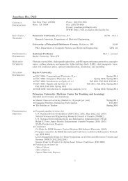
Fig. 6. Convergence of the shooting algorithm with the constraint
that the averaged pump power equals 20 mW for eight
pump waves and 100 signal waves. The pump waves are equally
spaced between 1430 and 1490 nm. The signal waves are equally
spaced between 1525 and 1605 nm with an input power of
−3 dBm per channel. (a) Average input pump power as a function
of iteration number. (b) Input pump power at z=L as a function
of iteration number.
Fig. 5. Convergence of the shooting algorithm with the constraint
that the averaged pump power equals 20 mW for four
pump waves with 50 signal waves. The pump waves are equally
spaced between 1437 and 1462 nm. The signal waves are equally
spaced between 1530 and 1570 nm with an input signal power of
−3 dBm per channel. (a) Average input pump power as a function
of iteration number. (b) Input pump power at z=L as a function
of iteration number.
pump power if the pump waves experience only the fiber
loss. Note that as the average pump powers converge to
the same value shown in Fig. 5(a), the input pump powers
at z=L converge to different values shown in Fig. 5(b), because
of pump-to-pump and pump-to-signal interactions.
In this simulation, the 50 signal waves are spaced equally
between 1530 and 1570 nm with an input signal power of
−3 dBm per channel. The output signal powers are between
−10 and −5.8 dBm. The pump waves are spaced
equally between 1437 and 1462 nm. From the simulation,
we obtain input pump powers between 137 mW and 263
mW, as shown in Fig. 5(b). Figure 6 shows the same convergence
for eight pump waves and 100 signal waves for
the same shooting target of 20 mW average pump power.
In this case, the continuation method was used in combination
with the shooting algorithm, since the algorithm
cannot converge for the desired 20 mW shooting target
with the initial guesses for the pumps obtained from the
fiber loss. Therefore the continuation method sets the
shooting target as 10 mW, following the flowchart in
Fig. 4, and after convergence at the fifth iteration, the
shooting target is reset to 20 mW. The initial guess for the
sixth iteration is determined from the converged pump
output power at z=0. In Fig. 6(a), the solid curve with