Modeling backward-pumped Raman amplifiers - Jonathan Hu ...
Modeling backward-pumped Raman amplifiers - Jonathan Hu ...
Modeling backward-pumped Raman amplifiers - Jonathan Hu ...

You also want an ePaper? Increase the reach of your titles
YUMPU automatically turns print PDFs into web optimized ePapers that Google loves.
<strong>Hu</strong> et al. Vol. 22, No. 10/October 2005 / J. Opt. Soc. Am. B 2083<br />
<strong>Modeling</strong> <strong>backward</strong>-<strong>pumped</strong> <strong>Raman</strong> <strong>amplifiers</strong><br />
<strong>Jonathan</strong> <strong>Hu</strong><br />
Department of Computer Science and Electrical Engineering, University of Maryland Baltimore County,<br />
Baltimore, Maryland 21250<br />
Brian S. Marks<br />
Department of Computer Science and Electrical Engineering, University of Maryland Baltimore County,<br />
Baltimore, Maryland, 21250; The Laboratory for Physical Sciences, 8050 Greenmead Dr.,<br />
College Park, Maryland 20740<br />
Qun Zhang<br />
Department of Electrical and Computer Engineering, University of Minnesota Duluth,<br />
271 Marshall W. Alworth Hall, 1023 University Dr., Duluth, Minnesota 55812<br />
Curtis R. Menyuk<br />
Department of Computer Science and Electrical Engineering, University of Maryland Baltimore County,<br />
Baltimore, Maryland 21250<br />
Received February 8, 2005; revised manuscript received May 4, 2005; accepted May 6, 2005<br />
We describe a robust shooting algorithm to model <strong>backward</strong>-<strong>pumped</strong> <strong>Raman</strong> <strong>amplifiers</strong>. This algorithm uses a<br />
continuation method and a Jacobi weight in conjunction with the shooting algorithm. We compare this algorithm<br />
to the commonly used relaxation algorithm. We find that the shooting algorithm is more flexible, in that<br />
it can be applied to <strong>amplifiers</strong> in which one fixes the gain, in contrast to the standard relaxation algorithm,<br />
which can be applied only to two-point boundary-value problems. However, it is less efficient when applied to<br />
two-point boundary-value problems, in that it requires more computer time. © 2005 Optical Society of<br />
America<br />
OCIS codes: 060.0060, 060.2320, 190.5650.<br />
1. INTRODUCTION<br />
Fiber <strong>Raman</strong> <strong>amplifiers</strong> have become important in recent<br />
years. By using multiple pumps, one can tailor the gain<br />
over a large bandwidth. Moreover, the gain is spatially<br />
distributed, leading to an improvement in the signal-tonoise<br />
ratio relative to systems that employ only erbiumdoped<br />
fiber <strong>amplifiers</strong>. 1 The power variation in <strong>backward</strong><strong>pumped</strong><br />
<strong>Raman</strong> <strong>amplifiers</strong> is described by a set of coupled<br />
differential equations that accounts for both fiber attenuation<br />
and the nonlinear coupling between waves due to<br />
stimulated <strong>Raman</strong> scattering. With forward pumping, it<br />
is not difficult to numerically solve these coupled equations<br />
using standard integration techniques. However,<br />
<strong>backward</strong> pumping complicates the problem, because the<br />
input signal powers are specified at one end of the fiber,<br />
whereas the input pump powers are specified at the other<br />
end. This two-point boundary-value problem is usually<br />
solved with an iterative scheme. 2<br />
When an algorithm for numerically solving a problem<br />
such as this two-point boundary-value problem is designed,<br />
the algorithm must possess the following characteristics:<br />
speed, accuracy, robustness, and flexibility.<br />
Speed refers to minimizing the amount of computer time<br />
needed to solve a given problem. Accuracy refers to the<br />
amount of the error associated with a given integration<br />
scheme or iterative method, given the integration step<br />
size and the number of iterations. Since the common<br />
methods for solving the <strong>Raman</strong> equations are iterative,<br />
one is concerned with whether the method converges. We<br />
say that a method is robust if it converges for a realistic<br />
range of parameters. Finally, a flexible method is an algorithm<br />
that can be applied to a large class of problems. In<br />
our context, a flexible method should be able to solve both<br />
the problem in which boundary values for the pumps are<br />
specified and the problem in which one fixes the gain of<br />
the <strong>Raman</strong> amplifier. Both conditions are important in<br />
practice.<br />
One of the most common approaches for solving the<br />
two-point boundary-value problem is to first integrate the<br />
signal waves forward using a fixed pump profile and then<br />
to integrate the pump waves <strong>backward</strong> using a fixed signal<br />
profile to ensure that both boundary conditions are<br />
automatically satisfied. This relaxation algorithm is then<br />
iterated until the solution converges. 3,4 The relaxation algorithm<br />
is fast and accurate, and for the problems we<br />
have considered (up to eight pump waves and 100 signal<br />
waves with a realistic set of parameters), it is robust.<br />
However, it is only applicable to two-point boundaryvalue<br />
problems. One often wants to fix the amplifier’s<br />
gain rather than the input pump power. In this case, one<br />
0740-3224/05/102083-8/$15.00 © 2005 Optical Society of America
2084 J. Opt. Soc. Am. B/ Vol. 22, No. 10/ October 2005 <strong>Hu</strong> et al.<br />
must specify the distance-integrated pump power rather<br />
than the boundary value, which is the input power. 5–7<br />
This problem is no longer a two-point boundary-value<br />
problem, and the relaxation algorithm is not flexible<br />
enough to handle it.<br />
In this paper, we describe the alternative approach of<br />
using a shooting algorithm to solve the propagation equations<br />
of <strong>Raman</strong> <strong>amplifiers</strong>. 2,8 Although this method has<br />
been presented previously in the literature, 9–11 we<br />
present extensions and details about the implementation<br />
of the shooting algorithm. We show that when applied appropriately,<br />
the shooting algorithm is as accurate and robust<br />
as the relaxation algorithm while being flexible<br />
enough to satisfy the constraint of fixed gain and, in principle,<br />
other constraints. 7 We show a comparison of two integration<br />
techniques combined with the shooting<br />
algorithm—the improved Euler method and the poweraverage<br />
method 3 —to investigate efficiency and convergence.<br />
We also investigate the use of a Jacobi weight and<br />
a continuation method, in which the pump powers are<br />
gradually increased to the desired values. Using the Jacobi<br />
weight and the continuation method in conjunction<br />
with the shooting algorithm yields a very robust algorithm<br />
for solving the <strong>Raman</strong> amplifier equations. However,<br />
using these extensions typically causes the shooting<br />
algorithm to be slower than the relaxation algorithm,<br />
when they can both be applied to the same problem.<br />
Hence, if one is solving a two-point boundary-value problem,<br />
one should use the relaxation method; whereas if one<br />
requires a different constraint, the shooting method is<br />
preferred.<br />
2. DESIGN ALGORITHM<br />
We describe wave propagation in a <strong>backward</strong>-<strong>pumped</strong>,<br />
multiple-wavelength fiber <strong>Raman</strong> amplifier using a<br />
system of coupled equations that includes the effects of<br />
spontaneous <strong>Raman</strong> scattering and Rayleigh<br />
backscattering. 3,12–16 The pump-to-pump, pump-to-signal,<br />
and signal-to-signal <strong>Raman</strong> interactions are considered in<br />
the coupled equations<br />
± dP m+n<br />
k<br />
dz =− kP k + g jk P j P k ,<br />
1a<br />
j=1<br />
where n is the number of pump waves and m is the number<br />
of signal waves. The values P k , k , and k describe, respectively,<br />
the power, frequency, and attenuation coefficient<br />
for the kth wave, where k=1,2,…,m+n. The<br />
quantities P ASE,k , P SRB,k , and P DRB,k are the powers corresponding<br />
to amplified spontaneous emission (ASE) noise,<br />
single Rayleigh backscattering (SRB), and double<br />
Rayleigh backscattering (DRB), respectively. The gain coefficient<br />
g jk describes the power transferred by stimulated<br />
<strong>Raman</strong> scattering between the jth and kth waves and<br />
is given by g jk =1/2A eff g j j − k for j k and g jk =<br />
−1/2A eff k / j g k k − j for j k , where g i is the<br />
<strong>Raman</strong> gain spectrum measured with respect to the pump<br />
frequency i , shown in Fig. 1 for silica fiber at the pump<br />
wavelength 0 =1 m, and A eff is the fiber effective area.<br />
The temperature-dependent term contributing to ASE<br />
noise is given by F jk =N phon +1 for j k , F jk =−N phon for<br />
j k , where N phon =exph j − k /k B T−1 −1 . Here, the<br />
parameters K, T, k B , and h are the Rayleigh backscattering<br />
coefficient, the temperature of the system, Boltzmann’s<br />
constant, and Planck’s constant, respectively. For<br />
a fiber span of length L, the boundary conditions are defined<br />
at z=0 for the signal waves P k 0=P k0 k<br />
=1,2,…,m, and at z=L for the <strong>backward</strong>-propagating<br />
pump waves P k L=P k0 k=m+1,m+2,…,m+n. In Eqs.<br />
(1a) and (1b), one uses the + sign for forward-propagating<br />
waves and the − sign for <strong>backward</strong>-propagating waves.<br />
Equations (1) are valid under the assumption that the<br />
gain in the <strong>Raman</strong> amplifier is due only to pump-to-signal<br />
and signal-to-signal <strong>Raman</strong> scattering. Therefore we neglect<br />
the <strong>Raman</strong> interaction of the ASE, SRB, and DRB<br />
with the pumps and signals, as this interaction is very<br />
small. Also, polarization effects have been neglected in<br />
Eqs. (1).<br />
Previous publications that describe the numerical<br />
implementation of the <strong>backward</strong>-<strong>pumped</strong> <strong>Raman</strong> ampli-<br />
± dP m+n<br />
ASE,k<br />
=− k P ASE,k +<br />
dz g jk P j P ASE,k + h k F jk ,<br />
j=1<br />
1b<br />
− dP m+n<br />
SRB,k<br />
=− k P SRB,k +<br />
dz g jk P j P SRB,k + KP k ,<br />
j=1<br />
1c<br />
dP DRB,k<br />
dz<br />
m+n<br />
=− k P DRB,k + g jk P j P DRB,k + KP SRB,k ,<br />
j=1<br />
1d<br />
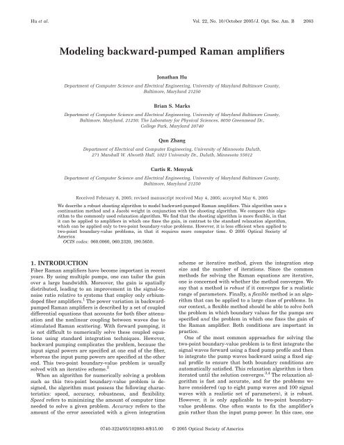
Fig. 1. (a) <strong>Raman</strong> gain spectrum g R of a typical silica fiber<br />
at the pump wavelength 0 =1 m. (b) Loss profile for a typical<br />
silica fiber.
<strong>Hu</strong> et al. Vol. 22, No. 10/October 2005 / J. Opt. Soc. Am. B 2085<br />
fier model use the relaxation algorithm, in which the ordinary<br />
differential equations (ODEs) corresponding to<br />
forward-propagating waves are decoupled from the ODEs<br />
corresponding to <strong>backward</strong>-propagating waves. 3,4 Each<br />
set of ODEs is then solved independently with the appropriate<br />
boundary conditions. With this algorithm, the<br />
boundary conditions are automatically satisfied, and the<br />
iteration is carried out until the entire system of ODEs is<br />
also satisfied to the desired accuracy. In this paper, we<br />
present a shooting algorithm, which is an alternative to<br />
the relaxation algorithm. Using the shooting algorithm,<br />
one solves all of the differential equations simultaneously<br />
in the forward direction using an estimate of the pump<br />
output powers. Thus the ODEs are automatically satisfied<br />
to the order of accuracy of the numerical integration<br />
scheme, and the iteration is carried out until the boundary<br />
conditions or some other shooting target is satisfied.<br />
No <strong>backward</strong> integration or decoupling of the system of<br />
ODEs is necessary. However, one must iterate the solution<br />
until the boundary conditions or other target conditions<br />
that specify the solution uniquely are satisfied.<br />
3. NUMERICAL MODEL AND SIMULATION<br />
OPTIMIZATION<br />
A. Shooting Algorithm<br />
The solution that we describe below solves only Eq. (1a).<br />
Usually, ASE, SRB, and DRB wave powers are small.<br />
Hence, they can be treated as perturbations. 15,17 In this<br />
case, ASE, SRB, and DRB can be included after Eq. (1a) is<br />
solved, since Eqs. (1b)–(1d) are decoupled from Eq. (1a).<br />
When one has a large <strong>Raman</strong> pump, Eqs. (1a)–(1d) can be<br />
solved together by using the iterative algorithm described<br />
in this paper. The ASE, SRB, and DRB waves can be considered<br />
as additional signal or pump waves according to<br />
their propagation direction with zero input power. 18 The<br />
two-point boundary-value problem may be stated mathematically<br />
as follows,<br />
dP<br />
= hP = A + GPP,<br />
dz 2<br />
=P0. Let P¯ 0 be an approximation to P 0 , and define P¯ z<br />
to be the solution of the initial value problem:<br />
dP¯<br />
dz = hP¯ , P¯ 0 = P¯ 0. 4<br />
Thus the variable P¯ satisfies the differential equations<br />
but not the correct boundary conditions. We define the<br />
vector<br />
fP¯ 0,P¯ L<br />
<br />
P 1 0 − P¯ 10<br />
0<br />
P 2 0 − P¯ 20<br />
0<br />
]<br />
]<br />
P m 0 − P¯ 0<br />
m0<br />
5<br />
P m+1 L − P¯ P m+1L<br />
]<br />
P m+n L − P¯ m+nL=<br />
m+1 L − P¯ m+1L<br />
]<br />
P m+n L − P¯ m+nL<br />
and note that the first m elements of vector f are zero.<br />
The last n elements of vector f are not zero in general,<br />
since the pump waves that we obtain from the numerical<br />
integration do not automatically satisfy the boundary<br />
conditions at L. Note that Eq. (5) is appropriate only for<br />
the case of the two-point boundary-value problem. We<br />
now construct the Jacobian matrices Q, M, and N, whose<br />
elements are defined as<br />
with the boundary conditions<br />
P k 0 = P k0<br />
k =1,2,…,m,<br />
Q ij = h i<br />
P j<br />
z, M ij = f i<br />
P j 0 , N ij = f i<br />
P j L ,<br />
6<br />
P k L = P k0 k = m +1,m +2,…,m + n, 3<br />
where P and h are vectors of length m+n, which is the<br />
total number of waves, A is the m+nm+n diagonal<br />
matrix responsible for the fiber attenuation, and GP is<br />
the m+nm+n matrix corresponding to the <strong>Raman</strong><br />
scattering terms in Eq. (1a). The example of the shooting<br />
algorithm that we present in this section uses integration<br />
from z=0 to z=L so that the pump input boundary conditions<br />
at z=L are the shooting “targets.” One can alternatively<br />
choose the shooting direction from z=L to z=0. The<br />
effectiveness of the shooting direction depends on the initial<br />
guess and other parameters. One can also modify the<br />
target for other applications, including in particular the<br />
constant gain criterion, which often appears in practice. 7<br />
The shooting algorithm that we implement is as follows:<br />
Let Pz be the true solution of Eq. (2), and let P 0<br />
for i, j=1,2,…,m+n. Note that in matrix M, the upper<br />
left mm block is the identity matrix. In matrix N, the<br />
lower right nn block is the identity matrix. Let Pz<br />
=Pz−P¯ z. Finding Pz is then equivalent to finding<br />
Pz so that<br />
dP¯ + P<br />
= hP¯ + P,<br />
dz<br />
fP¯ 0 + P0,P¯ L + PL<br />
=0. 7<br />
Expanding these expressions in a first-order Taylor series<br />
and using Eq. (4) yields the approximate formula
2086 J. Opt. Soc. Am. B/ Vol. 22, No. 10/ October 2005 <strong>Hu</strong> et al.<br />
d P<br />
= Q P, M P0 + N PL =−fP¯ 0,P¯ L.<br />
dz<br />
8<br />
The partial derivatives are to be evaluated for the approximate<br />
solution P¯ .<br />
We now describe an iterative procedure for determining<br />
P and hence P.<br />
1. Estimate the pumps’ boundary values at z=0. We<br />
first integrate the signal waves forward to get a signal<br />
profile assuming no pump wave. Then we integrate the<br />
pump waves <strong>backward</strong> using this signal profile. The<br />
pump power at z=0 will be a good initial guess to start<br />
the shooting iteration.<br />
2. Simultaneously integrate from z=0 to z=L,<br />
dP¯<br />
dU<br />
= QU<br />
dz<br />
U0 = I, 9a<br />
dz = hP¯ P¯ 0 = P¯ 0, 9b<br />
where I is the identity matrix of dimension m+n. We used<br />
the improved Euler method except as otherwise stated.<br />
This method is second-order accurate. 19 If we are solving<br />
the two-point boundary-value problem, then we know the<br />
signals’ boundary conditions at z=0, which means that m<br />
components of P0 are known. Therefore only nn+m<br />
elements in the matrix U must be calculated, instead<br />
of n+m 2 .<br />
3. Compute fP¯ 0,P¯ L.<br />
4. Solve the linear algebraic system MU0+NULS<br />
=−fP¯ 0,P¯ L. We used Gaussian elimination. 20 Then<br />
Pz=UzS satisfies the required Eq. (8), as may be<br />
verified by direct substitution.<br />
5. Obtain P 0 =U0S, which provides a correction to<br />
P¯ 0=P¯ 0. Replace P¯ 0 with P¯ 0+ P 0 for the pumps.<br />
6. Go to step 2, and iterate until solution converges.<br />
Again, to summarize our shooting algorithm, one must<br />
choose initial guesses for all pump-power values at the<br />
signal input side. Before the first shooting iteration, we<br />
integrate the ODEs by numerical integration from the<br />
signal input side to the signal output side under the assumption<br />
that there is no pump. Then we integrate the<br />
ODEs for the pump power from the signal output side to<br />
the signal input side with the signal-power values that we<br />
obtained from the first step. The pump-power values that<br />
we obtain at the signal input side are used as the initial<br />
guesses to start the shooting iteration. Then we integrate<br />
the coupled <strong>Raman</strong> equations for all signals and pumps in<br />
the forward direction.<br />
B. Average Pump-Power Model<br />
In Subsection 3.A, we described the shooting method to<br />
solve the two-point boundary-value problem. If one wants<br />
to solve the equations for the case of fixed average pump<br />
power, the algorithm is modified as follows.<br />
Equation (5) changes to<br />
1 0 − P¯ 10<br />
P 2 0 − P¯ 20<br />
]<br />
fP¯ 0,ĪP P m 0 − P¯ m0<br />
I m+1 − Ī m+1<br />
]<br />
I m+n − Ī m+n<br />
=I m+1 − Ī m+1<br />
0<br />
0<br />
]<br />
0<br />
]<br />
I m+n − Ī m+n,<br />
10<br />
where I j = 0 L P j zdz, j=m+1,m+2,…,m+n is the<br />
z-integrated pump power. Correspondingly, Eq. (6) must<br />
be changed to<br />
Q ij = h iz<br />
P j z , M ij = f i<br />
P j 0 ,<br />
Equation (7) changes to<br />
N ij = f i<br />
I j<br />
,<br />
11<br />
dP¯ + P<br />
= hP¯ + P, fP¯ 0 + P0,Ī + I =0,<br />
dz<br />
12<br />
where Ī= 0 L Pzdz. Similarly, expanding these expressions<br />
in a first-order Taylor series and using Eq. (4) yields<br />
the approximate formula<br />
d P<br />
dz = Q P, M P0 + N I =−fP¯ 0,Ī. 13<br />
Following the iterative procedure in Subsection 3.A, we<br />
need only to change steps 3, 4, and 5 to the following:<br />
3. Compute fP¯ 0,Ī, and Ū, where U ij = L 0 U ij zdz, i<br />
=m+1,m+2,…,m+n; j=1,2,…,m+n.<br />
4. Solve the linear algebraic system MU0+NŪS<br />
=−fP¯ 0,Ī.<br />
5. Obtain P 0 =U0S, which provides a correction to<br />
P¯ 0=P¯ 0. Replace P¯ 0 with P¯ 0+ P 0 for the pumps.<br />
After changing the above steps, the algorithm can then<br />
be used to solve the problem in which the distanceaveraged<br />
pump power is specified. 7<br />
C. Integration Method<br />
In the integration process, one solves the coupled <strong>Raman</strong><br />
equations by taking small steps in z using a numerical integration<br />
method, such as the improved Euler method.<br />
Another method that was recently described uses the average<br />
pump power in a z step, assuming an exponential<br />
variation in z. 3 We have found that this power-average<br />
method is also second-order accurate but is more complicated<br />
than the improved Euler method, since it requires<br />
the evaluation of exponential functions. In Fig. 2 we show<br />
the run time for the two integration schemes. We define<br />
the convergence parameter c as<br />
c =1<br />
nl i=1<br />
n l<br />
<br />
j=1<br />
P i r z j − P i r−1 z j <br />
P i r z j <br />
21/2<br />
, 14<br />
where the superscript r indicates the iteration number, l<br />
is the number of z steps used in the integration, and n is
<strong>Hu</strong> et al. Vol. 22, No. 10/October 2005 / J. Opt. Soc. Am. B 2087<br />
chosen appropriately for the problem. In Fig. 3, we plot<br />
the convergence parameter c versus iteration number for<br />
many values of and for the same simulation parameters<br />
as in Fig. 2. Figure 3 shows that the convergence rate<br />
changes considerably for different choices of . For some<br />
values, c decreases quite rapidly, indicating fast convergence,<br />
whereas for others there is no convergence. The<br />
choice of is problem dependent, and some experimentation<br />
is needed to find the optimum value.<br />
Fig. 2. Simulation time as a function of the z step size for different<br />
integration types with the threshold c=510 −4 . Squares<br />
denote the trapezoidal rule, and triangles denote the poweraverage<br />
method.<br />
Fig. 3. Convergence parameter c versus iteration number for<br />
different Jacobi weights .<br />
E. Continuation Method<br />
We have found that the algorithm that we present here<br />
sometimes has difficulty converging when the pump<br />
power is high. The value of the pump power that causes<br />
difficulty is problem dependent. For systems with 100 signal<br />
waves and eight pump waves using our fiber parameters,<br />
we found that this difficulty will occur when the<br />
pump power reaches 140 mW for every pump wave. For<br />
systems with 100 signal waves and two pump waves, we<br />
found that the algorithm has no problem until the pump<br />
power reaches 1900 mW for each pump wave. In our<br />
simulation, the signal powers are all set to 0.5 mW. To obtain<br />
convergence, we have used a continuation method in<br />
which the pump power is gradually raised to its desired<br />
value. When it is used in conjunction with a shooting algorithm,<br />
the continuation method therefore allows us to<br />
solve problems that do not converge with the shooting algorithm<br />
alone. 21 Figure 4 shows a block diagram of our<br />
implementation of the continuation method. Let P¯ desireL<br />
be the set of desired pump input powers and suppose that<br />
the shooting algorithm fails to converge. If the shooting<br />
algorithm converges for a set of pump values P¯ tryL<br />
=P¯ desireL, we wish to slowly increase to1inaway<br />
that the shooting converges. We follow the algorithm<br />
shown in Fig. 4 for choosing the value of . In every step,<br />
the number of pumps. We have carried out a simulation of<br />
eight pumps and 100 signals that iterates until a c=5<br />
10 −4 is achieved. Figure 2 shows that for the same accuracy,<br />
the two integration methods have very similar run<br />
times. Since the improved Euler method is simpler, we<br />
conclude that it is to be preferred.<br />
D. Weighted Jacobi Method<br />
For all the problems to which we applied the relaxation<br />
method, up to eight pump waves and 100 signal waves,<br />
we found that this method converges without any problem.<br />
By contrast, we found that in order for the shooting<br />
method to converge, we have to supplement it with a Jacobi<br />
weight, . Given a vector of pump output powers<br />
from the rth iteration, P 0 r at z=0, the shooting algorithm<br />
provides a new vector of pump output powers at z=0 for<br />
the next iteration, P 0 r+1 , that attempts to correct for the<br />
error. Rather than using P 0 r+1 directly, we define<br />
P r+1 0,J = 1−P r r+1<br />
0 + P 0<br />
15<br />
and use P r+1 0,J<br />
as the vector of pump powers at z=0 for the<br />
next iteration. Note that =1 corresponds to the direct<br />
usage of the result of the shooting algorithm. This technique<br />
speeds the convergence of the iteration when is<br />
Fig. 4.<br />
Block diagram of the continuation method.
2088 J. Opt. Soc. Am. B/ Vol. 22, No. 10/ October 2005 <strong>Hu</strong> et al.<br />
the initial choice for the pump powers for the <strong>Raman</strong> iteration<br />
at a new comes from the previous iteration.<br />
4. RESULTS AND COMPARISON<br />
In this section, we compare the run time for the relaxation<br />
and shooting algorithms to solve the two-point<br />
boundary-value problem. As an example, in a system of<br />
length L=50 km with one pump wave and 10 signal<br />
waves, the shooting algorithm is about four times slower<br />
than the relaxation algorithm. For a system with eight<br />
pump waves and 100 signal waves, the shooting algorithm<br />
is about nine times slower than the relaxation algorithm.<br />
The shooting algorithm is slower because of its<br />
complexity and the extensions required for convergence.<br />
However, as we pointed out, the shooting algorithm is<br />
more flexible in that it can solve the <strong>Raman</strong> equations under<br />
the constraint of specified averaged pump power. In<br />
Fig. 5, we show the convergence of the shooting algorithm<br />
when four pump waves are constrained to have a<br />
distance-averaged power of 20 mW, with 50 signal waves.<br />
The initial guesses to start the shooting algorithm are the<br />
pump output powers at z=0 that give 20 mW average<br />
Fig. 6. Convergence of the shooting algorithm with the constraint<br />
that the averaged pump power equals 20 mW for eight<br />
pump waves and 100 signal waves. The pump waves are equally<br />
spaced between 1430 and 1490 nm. The signal waves are equally<br />
spaced between 1525 and 1605 nm with an input power of<br />
−3 dBm per channel. (a) Average input pump power as a function<br />
of iteration number. (b) Input pump power at z=L as a function<br />
of iteration number.<br />
Fig. 5. Convergence of the shooting algorithm with the constraint<br />
that the averaged pump power equals 20 mW for four<br />
pump waves with 50 signal waves. The pump waves are equally<br />
spaced between 1437 and 1462 nm. The signal waves are equally<br />
spaced between 1530 and 1570 nm with an input signal power of<br />
−3 dBm per channel. (a) Average input pump power as a function<br />
of iteration number. (b) Input pump power at z=L as a function<br />
of iteration number.<br />
pump power if the pump waves experience only the fiber<br />
loss. Note that as the average pump powers converge to<br />
the same value shown in Fig. 5(a), the input pump powers<br />
at z=L converge to different values shown in Fig. 5(b), because<br />
of pump-to-pump and pump-to-signal interactions.<br />
In this simulation, the 50 signal waves are spaced equally<br />
between 1530 and 1570 nm with an input signal power of<br />
−3 dBm per channel. The output signal powers are between<br />
−10 and −5.8 dBm. The pump waves are spaced<br />
equally between 1437 and 1462 nm. From the simulation,<br />
we obtain input pump powers between 137 mW and 263<br />
mW, as shown in Fig. 5(b). Figure 6 shows the same convergence<br />
for eight pump waves and 100 signal waves for<br />
the same shooting target of 20 mW average pump power.<br />
In this case, the continuation method was used in combination<br />
with the shooting algorithm, since the algorithm<br />
cannot converge for the desired 20 mW shooting target<br />
with the initial guesses for the pumps obtained from the<br />
fiber loss. Therefore the continuation method sets the<br />
shooting target as 10 mW, following the flowchart in<br />
Fig. 4, and after convergence at the fifth iteration, the<br />
shooting target is reset to 20 mW. The initial guess for the<br />
sixth iteration is determined from the converged pump<br />
output power at z=0. In Fig. 6(a), the solid curve with
<strong>Hu</strong> et al. Vol. 22, No. 10/October 2005 / J. Opt. Soc. Am. B 2089<br />
squares shows the evolution for the pump with the shortest<br />
wavelength that needs the highest input pump power<br />
to yield the same average pump power. In this simulation,<br />
100 signal waves are spaced equally between 1525 and<br />
1605 nm with an input power of −3 dBm per channel. The<br />
output signal power is between 0.72 and −6.8 dBm. The<br />
pump waves are spaced equally between 1430 and 1490<br />
nm. The input pump powers obtained from the simulation<br />
are between 49 and 399 mW. Setting a larger target<br />
power will result in more iterations of the continuation<br />
method illustrated in Fig. 4. The threshold of c=110 −3<br />
was the convergence criterion used to finish the iteration<br />
when generating Figs. 5 and 6. The <strong>Raman</strong> gain and loss<br />
profile that we used are shown in Fig. 1.<br />
5. VALIDATION<br />
To validate our code, we have compared our simulation results<br />
with other published results. 4 Figure 7 shows the<br />
power evolution of the <strong>backward</strong>-propagating pumps for a<br />
system with eight pump waves and 100 signal waves, using<br />
the relaxation algorithm and the shooting algorithm.<br />
The parameters that we used—<strong>Raman</strong> gain, loss, pump<br />
wavelength, pump power, signal wavelength, and signal<br />
power—are inferred from the description in Ref. 4. The<br />
threshold of c=510 −4 was the convergence criterion<br />
used to stop the iteration for both the relaxation algorithm<br />
and the shooting algorithm, and hence both methods<br />
are able to achieve the same level of accuracy. The<br />
pump evolution shown in Fig. 7 yields good agreement<br />
with Fig. 5 of Ref. 4. Because this problem can be solved<br />
using both algorithms, we also compared the run time of<br />
the two algorithms. We found that the relaxation algorithm<br />
solves this problem in about 14 s on an Intel Pentium<br />
III 700 MHz machine, while the same problem using<br />
the shooting algorithm takes about 150 s. Hence, the run<br />
time is about 11 times slower for the shooting algorithm.<br />
In the example that we used in Section 4, which had<br />
lower pump power and signal gain, we found that the<br />
shooting algorithm is about nine times slower than the relaxation<br />
algorithm. The run time ratio is problem dependent,<br />
although we expect the shooting algorithm to generally<br />
be slower.<br />
We have demonstrated the shooting algorithm’s<br />
flexibility—and in particular its ability to handle the constraint<br />
of a specified average pump power—by its successful<br />
application to a genetic algorithm in which the pump<br />
spacing was optimized to minimize the gain ripple. 7 We<br />
validated it at the time by comparison to previously published<br />
results by Perlin and Winful. 5 Finally, we have also<br />
compared our simulation results for signal and noise with<br />
experimental data in our work in Ref. 22. All of these comparisons<br />
show good agreement.<br />
6. CONCLUSION<br />
To summarize, we present a multiple shooting algorithm<br />
for solving the <strong>Raman</strong> amplifier equations. We have<br />
shown that in conjunction with the continuation method,<br />
the shooting algorithm with the improved Euler integration<br />
method and a Jacobi weight is a robust algorithm for<br />
this problem. However, the shooting method is typically<br />
slower than the relaxation method because of these extensions.<br />
Hence, when one is solving a two-point boundaryvalue<br />
problem, the relaxation method should be used. On<br />
the other hand, the shooting method is more flexible than<br />
the commonly used relaxation method, as it can solve the<br />
<strong>Raman</strong> equations subject to a wide variety of constraints,<br />
including the constraint of fixed gain, rather than being<br />
restricted to two-point boundary-value problems.<br />
ACKNOWLEDGMENTS<br />
This work is supported by the U.S. Department of Energy<br />
and the National Science Foundation.<br />
J. <strong>Hu</strong>, the corresponding author, can be reached by<br />
e-mail at hu1@umbc.edu.<br />
Fig. 7. Power evolution of the <strong>backward</strong>-propagating pumps. (a)<br />
Result using the relaxation algorithm. (b) Result using the shooting<br />
algorithm. The threshold of c=510 −4 was the convergence<br />
criterion used to stop the iteration for both algorithms.<br />
REFERENCES<br />
1. S. Namiki and Y. Emori, “Ultrabroad-band <strong>Raman</strong><br />
<strong>amplifiers</strong> <strong>pumped</strong> and gain-equalized by wavelengthdivision-multiplexed<br />
high-power laser diodes,” IEEE J. Sel.<br />
Top. Quantum Electron. 7, 3–16 (2001).<br />
2. H. B. Keller, Numerical Methods for Two-Point Boundary-<br />
Value Problems (Ginn and Blaisdell, 1968).<br />
3. B. Min, W. J. Lee, and N. Park, “Efficient formulation of<br />
<strong>Raman</strong> amplifier propagation equations with average
2090 J. Opt. Soc. Am. B/ Vol. 22, No. 10/ October 2005 <strong>Hu</strong> et al.<br />
power analysis,” IEEE Photonics Technol. Lett. 12,<br />
1486–1488 (2000).<br />
4. H. Kidorf, K. Rottwitt, M. Nissov, M. Ma, and E.<br />
Rabarijanona, “Pump interactions in a 100-nm bandwidth<br />
<strong>Raman</strong> amplifier,” IEEE Photonics Technol. Lett. 11,<br />
530–532 (1999).<br />
5. V. Perlin and H. Winful, “Optimal design of flat-gain wideband<br />
fiber <strong>Raman</strong> <strong>amplifiers</strong>,” J. Lightwave Technol. 20,<br />
250–254 (2002).<br />
6. V. Perlin and H. Winful, “On distributed <strong>Raman</strong><br />
amplification for ultrabroadband long-haul WDM system,”<br />
J. Lightwave Technol. 20, 409–416 (2002).<br />
7. J. <strong>Hu</strong>, B. S. Marks, and C. R. Menyuk, “Flat-gain fiber<br />
<strong>Raman</strong> <strong>amplifiers</strong> using equally spaced pumps,” J.<br />
Lightwave Technol. 22, 1519–1522 (2004).<br />
8. D. D. Morrison, J. D. Riley, and J. F. Zancanaro, “Multiple<br />
shooting method for two-point boundary value problems,”<br />
Commun. ACM 5, 613–614 (1962).<br />
9. X. Liu and B. Lee, “Effective shooting algorithm and its<br />
application to fiber <strong>amplifiers</strong>,” Opt. Express 11, 1452–1461<br />
(2003).<br />
10. X. Liu and B. Lee, “A fast and stable method for <strong>Raman</strong><br />
amplifier propagation equations,” Opt. Express 11,<br />
2163–2176 (2003).<br />
11. X. Liu, “Powerful solution for simulating nonlinear coupled<br />
equations describing bidirectionally <strong>pumped</strong> broadband<br />
<strong>Raman</strong> <strong>amplifiers</strong>,” Opt. Express 12, 545–550 (2004).<br />
12. S. A. E. Lewis, S. V. Chernikov, and J. R. Taylor,<br />
“Temperature-dependent gain and noise in fiber <strong>Raman</strong><br />
<strong>amplifiers</strong>,” Opt. Lett. 24, 1823–1825 (1999).<br />
13. K. Rottwitt, M. Nissov, and F. Kerfoot, “Detailed analysis of<br />
<strong>Raman</strong> <strong>amplifiers</strong> for long-haul transmission,” in Optical<br />
Fiber Communication Conference (Optical Society of<br />
America, 1998), paper TuG1.<br />
14. S. E. Miller and A. G. Chynoweth, Optical Fiber<br />
Telecommunications (Academic, 1979).<br />
15. J. Bromage, “<strong>Raman</strong> amplification for fiber communication<br />
systems,” J. Lightwave Technol. 22, 79–93 (2002).<br />
16. X. Liu, J. Chen, C. Lu, and X. Zhou, “Optimizing gain<br />
profile and noise performance for distributed fiber <strong>Raman</strong><br />
<strong>amplifiers</strong>,” Opt. Express 12, 6053–6066 (2004).<br />
17. A. H. Hartog and M. P. Gold, “On the theory of<br />
backscattering in single-mode optical fibers,” J. Lightwave<br />
Technol. LT-2, 76–82 (1984).<br />
18. P. B. Hansen, L. Eskildsen, A. J. Stentz, T. A. Strasser, J.<br />
Judkins, J. J. DeMarco, R. Pedrazzani, and D. J.<br />
DiGiovanni, “Rayleigh scattering limitations in distributed<br />
<strong>Raman</strong> pre-<strong>amplifiers</strong>,” IEEE Photonics Technol. Lett. 10,<br />
159–161 (1998).<br />
19. W. E. Boyce and R. C. DiPrima, Elementary Differential<br />
Equations and Boundary Value Problems, 6th ed. (Wiley,<br />
1997).<br />
20. G. Strang, Linear Algebra and Its Applications, 3rd ed.<br />
(Harcourt College Publishers, 1988).<br />
21. S. M. Roberts and J. S. Shipman, Two-Point Boundary<br />
Value Problems: Shooting Methods (Elsevier, 1972).<br />
22. G. E. Tudury, J. <strong>Hu</strong>, B. S. Marks, G. M. Carter, and C. R.<br />
Menyuk, “Spectral gain characteristics of an amplified<br />
hybrid <strong>Raman</strong>/EDFA 210 km link,” in Conference on Laser<br />
and Electro Optics (Optical Society of America, 2003),<br />
paper CThM52.