Simulation of Ship Motion in Seaway - Automation
Simulation of Ship Motion in Seaway - Automation
Simulation of Ship Motion in Seaway - Automation

Create successful ePaper yourself
Turn your PDF publications into a flip-book with our unique Google optimized e-Paper software.
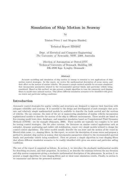
<strong>Simulation</strong> <strong>of</strong> <strong>Ship</strong> <strong>Motion</strong> <strong>in</strong> <strong>Seaway</strong><br />
by<br />
Tristan Pérez † and Mogens Blanke‡<br />
Technical Report EE02037<br />
Dept. <strong>of</strong> Electrical and Computer Eng<strong>in</strong>eer<strong>in</strong>g<br />
The University <strong>of</strong> Newcastle, NSW, 2308, Australia<br />
‡Section <strong>of</strong> <strong>Automation</strong> at Ørsted.DTU<br />
Technical University <strong>of</strong> Denmark, Build<strong>in</strong>g 326<br />
DK-2800 Kgs. Lyngby, Denmark<br />
Abstract<br />
Accurate modell<strong>in</strong>g and simulation <strong>of</strong> ship motion <strong>in</strong> seaway is essential to test applications <strong>of</strong> ship<br />
motion control strategies. In this report, we review the mathematical description <strong>of</strong> ocean waves, and<br />
their effect on the motion <strong>of</strong> mar<strong>in</strong>e vehicles. We present a simple method suitable for accurate simulation<br />
that <strong>in</strong>corporates parameters related to the recommended spectral family and particular vehicle be<strong>in</strong>g<br />
considered. Based on this method, we also present a simple algorithm to tune the commonly used shap<strong>in</strong>g<br />
filters to model wave <strong>in</strong>duced motion. This allows different simulation scenarios to be identified with given<br />
sea states and particular sail<strong>in</strong>g conditions.<br />
Introduction<br />
Automatic control strategies for mar<strong>in</strong>e vehicles and structures are designed to improve their functions with<br />
adequate reliability and economy. It is essential to the design and development <strong>of</strong> such strategies that accurate<br />
and relatively simple mathematical models be available to describe the loads exerted and the motions<br />
<strong>of</strong> vehicles. On one extreme, the state <strong>of</strong> the art <strong>in</strong> maneuver<strong>in</strong>g simulation <strong>of</strong> mar<strong>in</strong>e vehicles <strong>in</strong>corporates<br />
sophisticated models to describe the motion <strong>of</strong> the ship <strong>in</strong> different environments. These models are based on<br />
free-runn<strong>in</strong>g model tests data, databases, and numerical simulation based on Computational Fluid Dynamics<br />
Methods (CFDM)—see for example (Simonsen, 2000). These models are typically too complex to be used<br />
for test<strong>in</strong>g control strategies. On the other extreme, the literature on mar<strong>in</strong>e control applications such as<br />
autopilot, dynamic position<strong>in</strong>g and rudder roll stabilization, report very simple models utilized to design the<br />
control control algorithms. The latter models usually describe the sea state and the motion <strong>of</strong> the vessel by<br />
filtered white noise, i.e., shap<strong>in</strong>g filters. In this report, we review the description <strong>of</strong> ocean waves and propose a<br />
method to simulate ship motion <strong>in</strong> seaway that <strong>in</strong>corporates parameters related to the recommended spectral<br />
family and particular vehicle be<strong>in</strong>g considered. Then we present a simple algorithm to tune shap<strong>in</strong>g filters<br />
that allows different simulation scenarios to be readily identified with given sea states and particular sail<strong>in</strong>g<br />
conditions.<br />
The rest <strong>of</strong> the report is organized as follows. In section 1, we <strong>in</strong>troduce the stochastic mathematical models<br />
for describ<strong>in</strong>g sea states, and their properties. In section 2, we describe the relations between the sea elevation<br />
and ship motion components giv<strong>in</strong>g a stochastic mathematical description <strong>of</strong> the phenomena. In section 3, we<br />
present a simple algorithm to tune shap<strong>in</strong>g filters and we show some simulation results. F<strong>in</strong>ally, <strong>in</strong> section 4,<br />
we summarize and discuss the presented material.<br />
1
1 Stochastic description <strong>of</strong> irregular seas<br />
Ocean waves are random <strong>in</strong> terms <strong>of</strong> both time and space. Therefore, a stochastic modell<strong>in</strong>g description seems<br />
to be the most appropriate approach to describe them—see for example St Denis and Pierson (1953).<br />
In practice, it is assumed that the variations <strong>of</strong> the stochastic characteristics <strong>of</strong> the sea are much slower<br />
than the variations <strong>of</strong> the sea surface itself. Due to this, the elevation <strong>of</strong> the sea at a position x, y, denoted by<br />
ζ(x, y, t), can be considered a realization <strong>of</strong> a stationary process. The follow<strong>in</strong>g simplify<strong>in</strong>g assumptions about<br />
the underly<strong>in</strong>g stochastic model are usually made (Haverre and Moan, 1985):<br />
• The observed sea surface, at a certa<strong>in</strong> location and for short periods <strong>of</strong> time, is considered a realization<br />
<strong>of</strong> a stationary and homogeneous, zero mean Gaussian stochastic process.<br />
• Some standard formulae for the spectral density function S(ω) are adopted.<br />
Under a Gaussian assumption, the process, <strong>in</strong> a statistical sense, is completely characterized by the power<br />
spectral density function S(ω).<br />
The validity <strong>of</strong> this hypothesis <strong>of</strong> stationarity and Gaussianity, have been <strong>in</strong>vestigated via extensive analysis<br />
<strong>of</strong> time series recorded from wave rid<strong>in</strong>g buoys <strong>in</strong> the North Atlantic Ocean Haverre and Moan (1985). In<br />
this study, It has been reported that:<br />
• For low and moderate sea states (Significant wave height 1 h 1/3 < 4m), the sea can be considered<br />
stationary for periods over 20 m<strong>in</strong>. For more severe sea states, stationarity can be questioned even for<br />
periods <strong>of</strong> 20 m<strong>in</strong>.<br />
• For low to medium states (h 1/3 < 8m), Gaussian models are still accurate, but deviations from Gaussianity<br />
slightly <strong>in</strong>crease with the <strong>in</strong>creas<strong>in</strong>g severity <strong>of</strong> the sea state.<br />
Model to describe the sea elevation<br />
A conceptual model to describe the elevation <strong>of</strong> an irregular sea is given by the sum <strong>of</strong> a large number <strong>of</strong><br />
essentially <strong>in</strong>dependent regular (s<strong>in</strong>usoidal) contributions with random phases. In this representation, the sea<br />
elevation at a location x, y with respect to an <strong>in</strong>ertial reference frame is given by<br />
N�<br />
N�<br />
ζ(x, y, t) = ζi(x, y, t) = ζi cos (kix cos χ + kiy s<strong>in</strong> χ + ωit + θi) , (1)<br />
i=0<br />
i=0<br />
where ζi(x, y, t) is the contribution <strong>of</strong> the regular or harmonic travell<strong>in</strong>g wave components i progress<strong>in</strong>g at an<br />
angle χ with respect to the <strong>in</strong>ertial frame and a with random phase θi. The parameters ki (wave number), ωi<br />
(wave frequency seen from a fixed position), ζ i (constant wave amplitude) characterize each component. For<br />
each realization, the phase θi <strong>of</strong> each components is chosen to be a random variable with uniform distribution<br />
on the <strong>in</strong>terval [−π, π]. This choice ensures the stationarity <strong>of</strong> ζ(x, y, t) (Gelb and Velde, 1968).<br />
For each regular wave component i, the phase velocity, ci, is the velocity with which the wave crest move<br />
relative to ground. Assum<strong>in</strong>g <strong>in</strong>f<strong>in</strong>ite depth <strong>of</strong> water, the follow<strong>in</strong>g relations hold<br />
�<br />
gλi<br />
ci =<br />
2π ; ki = 2π<br />
; ωi =<br />
λi<br />
√ gki = g<br />
(2)<br />
ci<br />
where λi is the wavelength <strong>of</strong> the component i. The last expression is known as the dispersion <strong>of</strong> gravity waves,<br />
and establishes that the phase velocity is <strong>in</strong>versely proportional to its frequency. This means that long waves<br />
propagate faster than short ones. This phenomenon is important for simulat<strong>in</strong>g ship motion <strong>in</strong> waves as we<br />
shall see <strong>in</strong> the follow<strong>in</strong>g sections <strong>of</strong> the report: a ship advanc<strong>in</strong>g <strong>in</strong> a seaway <strong>in</strong> follow<strong>in</strong>g seas will overtake<br />
some short waves, while it will be overtaken by some long ones.<br />
For simplicity, let us consider the case <strong>in</strong> which the observations are made at the orig<strong>in</strong> <strong>of</strong> the reference<br />
1Thesignificantwaveheighth1/3is related to the w<strong>in</strong>d speed and it is def<strong>in</strong>ed as the average <strong>of</strong> one third <strong>of</strong> the highest<br />
observations <strong>of</strong> the wave amplitude (Price and Bishop, 1974), i.e., h1/3 � 3 � Highest one third <strong>of</strong> the sampled waves<br />
.<br />
Total number <strong>of</strong> sampled waves<br />
2
frame, and that the waves come from angle <strong>of</strong> <strong>in</strong>cidence χ = 0 with respect to the reference frame. The<br />
amplitude <strong>of</strong> the wave components, is then conveniently def<strong>in</strong>ed <strong>in</strong> terms <strong>of</strong> a adopted local power spectral<br />
density S(w) satisfy<strong>in</strong>g<br />
� ∞<br />
var[ζ(t)] = S(ω)dω. (3)<br />
Thus, for the case considered, the model <strong>of</strong> the seas elevation (1) becomes<br />
i=0<br />
0<br />
N�<br />
N�<br />
ζ(t) = ζi(t) = ζi cos(ωit + θi), (4)<br />
i=0<br />
where at any particular wave frequency ωi, the variance <strong>of</strong> that component with<strong>in</strong> a band ∆ω centered at ωi<br />
is approximated by<br />
var[ζi(t)] = 1<br />
2 ζi<br />
� ∆ω ωi+<br />
2 2<br />
≈<br />
ωi− ∆ω<br />
S(ω)dω. (5)<br />
2<br />
The amplitudes <strong>of</strong> wave components can be approximated by<br />
�<br />
�<br />
� � ∆ω ωi+ 2<br />
ζi ≈<br />
�<br />
2 S(ω) dω. (6)<br />
ωi− ∆ω<br />
2<br />
Recommended spectra for fully-developed long-crested seas<br />
In any particular sea state, the elevation <strong>of</strong> the ocean surface presents irregular characteristics. After the w<strong>in</strong>d<br />
has blown constantly for a certa<strong>in</strong> period <strong>of</strong> time the sea elevation becomes statistically stable. In this case,<br />
the sea is referred to as fully-developed. If the irregularity <strong>of</strong> the observed waves are only <strong>in</strong> the dom<strong>in</strong>ant w<strong>in</strong>d<br />
direction so that there are ma<strong>in</strong>ly uni-directional wave crests with vary<strong>in</strong>g separation and rema<strong>in</strong><strong>in</strong>g parallel<br />
to each other the sea is referred to as a long-crested irregular sea (Price and Bishop, 1974).<br />
Based on extensive data collection, mostly <strong>in</strong> the North Atlantic ocean, a series <strong>of</strong> idealized s<strong>in</strong>gle side local<br />
spectra have been obta<strong>in</strong>ed to described long-crested seas. For example, for fully-developed seas the<br />
one-parameter Pierson-Moskowits (PM) spectrum is given by—see for example (Price and Bishop, 1974):<br />
SPM (ω) = 0.78<br />
ω5 � �<br />
exp<br />
−3.11<br />
(m 2 sec), (7)<br />
ω 4 h 2 1/3<br />
<strong>in</strong> which the ma<strong>in</strong> parameter is the significant wave height, h 1/3. The peak frequency <strong>of</strong> the PM spectrum is<br />
ω0 =1.26 h −1/2<br />
1/3 . (8)<br />
For prediction <strong>of</strong> the responses <strong>of</strong> mar<strong>in</strong>e vehicles and <strong>of</strong>fshore structures, The 2nd International <strong>Ship</strong> and<br />
Offshore Structures Congress (ISSC, 1964) and 12th and 15th International Tow<strong>in</strong>g Tank Conference (ITTC,<br />
1969, 1978) recommended the use <strong>of</strong> a Modified Pierson-Moskowits (MPM) spectrum. When SI units are used,<br />
this has the form:<br />
SMPM (ω) = 4π3 h 2 1/3<br />
ω 5 T 4<br />
� � 3 −16π<br />
exp<br />
ω 4 T 4<br />
(m 2 sec), (9)<br />
<strong>in</strong> which the ma<strong>in</strong> parameters are the significant wave height, h 1/3 and the dom<strong>in</strong>ant wave period T . The<br />
period correspond<strong>in</strong>g to peak frequency <strong>of</strong> the spectrum is given by<br />
T0 =1.408 T. (10)<br />
This spectrum should be used to simulate fully developed seas with <strong>in</strong>f<strong>in</strong>ite depth, no swell and unlimited<br />
fetch 2 (Fossen, 1994). For cases <strong>in</strong> which geographical boundaries limit the fetch, the so-called JONSWAP<br />
(Jo<strong>in</strong> North Sea Wave Project) is recommended—see for example, (Lewis, 1988), (Falt<strong>in</strong>sen, 1990) and references<br />
there<strong>in</strong>.<br />
2 Fetch is the distance between the po<strong>in</strong>t at which the waves are observed and a w<strong>in</strong>dward boundary, such as a shore or the<br />
edge <strong>of</strong> a storm area. The fetch gives a notion <strong>of</strong> the area <strong>of</strong> <strong>in</strong>teraction between the w<strong>in</strong>d and sea surface with respect to the<br />
observation po<strong>in</strong>t.<br />
3
Figure 1 shows the form <strong>of</strong> PM and MPM spectra for different significant wave heights. The significant<br />
wave height can be larger than 2m for 60% <strong>of</strong> the time <strong>in</strong> hostile areas such as the North Sea and reach<br />
20m <strong>in</strong> extreme conditions with average w<strong>in</strong>ds over 60kts (Price and Bishop, 1974). The mean period can<br />
be between 4sec and 20sec, but is usually not below that (Falt<strong>in</strong>sen, 1990). Figure 2 shows the value <strong>of</strong> the<br />
SPM[m 2 s]<br />
SMPM[m 2 s]<br />
7<br />
6<br />
5<br />
4<br />
3<br />
2<br />
1<br />
h 1/3 =2m<br />
h 1/3 =4m<br />
h 1/3 =6m<br />
0<br />
0 0.2 0.4 0.6 0.8 1 1.2 1.4 1.6 1.8 2<br />
6<br />
5<br />
4<br />
3<br />
2<br />
1<br />
PM Spectrum<br />
ω<br />
MPM Spectrum for T = 7 sec.<br />
h 1/3 =2m<br />
h 1/3 =4m<br />
h 1/3 =6m<br />
0<br />
0 0.2 0.4 0.6 0.8 1 1.2 1.4 1.6 1.8 2<br />
Figure 1: PM spectrum and recommended MPM by ITTC and ISSC for different significant wave height h 1/3.<br />
regular amplitude components calculated us<strong>in</strong>g (6) for MPM spectrum for a given vector <strong>of</strong> frequencies. This<br />
figure also shows a particular realization <strong>of</strong> the sea elevation ζ(t) determ<strong>in</strong>ed us<strong>in</strong>g (4) with a vector <strong>of</strong> random<br />
phases uniformly distributed on [−π, π].<br />
Short-crested seas<br />
When irregularities are apparent along the wave crests at right angles to the direction <strong>of</strong> the w<strong>in</strong>d, the sea<br />
is referred to as short-crested irregular sea or confused sea (Price and Bishop, 1974). Short-crestedness is<br />
characteristic <strong>of</strong> locations closer to storm areas due to the angular dispersion or spread<strong>in</strong>g <strong>of</strong> many wave<br />
systems com<strong>in</strong>g from different directions. In a short-crested sea, the waves approach the vessel or mar<strong>in</strong>e<br />
structure from a variety <strong>of</strong> directions χ with a ma<strong>in</strong> direction <strong>of</strong> propagation χ0. For this case, a directional<br />
spectrum tak<strong>in</strong>g <strong>in</strong>to account the different directions <strong>of</strong> the components gives a more accurate description.<br />
The elevation <strong>of</strong> the sea surface is then described by,<br />
where,<br />
ζ(t) =<br />
N�<br />
i=0 j=0<br />
� ∞<br />
var[ζ(t)] =<br />
ω<br />
M�<br />
ζij cos[−ωit + θij] (11)<br />
0<br />
� π<br />
−π<br />
S(ω, α)dαdω. (12)<br />
In which, S(ω, α) is a so-called directional or two-dimensional spectrum (Price and Bishop, 1974), with α �<br />
χ − χ0, and<br />
�<br />
ζij ≈ 2S(ωi,αj)∆α∆ω. (13)<br />
S<strong>in</strong>ce the measurement <strong>of</strong> directional spectra is, <strong>in</strong> general, very difficult, <strong>in</strong> most applications, it is sufficient<br />
to assume that S(ω, α) can be factorized as S(ω, α) =S(ω)M(α). The factor M(α) is called the spread<strong>in</strong>g<br />
4
ζi[m]<br />
ζ[m]<br />
0.5<br />
0.4<br />
0.3<br />
0.2<br />
0.1<br />
0<br />
0 0.2 0.4 0.6 0.8 1 1.2 1.4 1.6 1.8 2<br />
3<br />
2<br />
1<br />
0<br />
−1<br />
−2<br />
MPM h 1/3 =4andT =7sec.<br />
ω<br />
−3<br />
0 20 40 60 80 100 120 140 160 180 200<br />
Figure 2: Amplitude <strong>of</strong> regular wave components ζi calculated us<strong>in</strong>g MPM with h 1/3 =4andT =7sec, and<br />
a particular realization. height h 1/3.<br />
t[sec]<br />
function. The usually adopted (and recommended by ITTC) spread<strong>in</strong>g function is given by<br />
M(α) =<br />
2 <strong>Ship</strong>motion<strong>in</strong><strong>Seaway</strong><br />
� 2cos 2 (α)<br />
π<br />
if −π/2 � α � π/2,<br />
0 otherwise.<br />
The response <strong>of</strong> a ship to waves is very complex. Hav<strong>in</strong>g a certa<strong>in</strong> velocity <strong>of</strong> advance, a ship experiences the<br />
wave excitation at an encounter frequency. As we will see, this frequency is not related l<strong>in</strong>early to the wave<br />
frequency, as seen from a fixed po<strong>in</strong>t, but varies with ship speed and predom<strong>in</strong>ant direction between waves <strong>in</strong><br />
a nonl<strong>in</strong>ear fashion.<br />
Frequency <strong>of</strong> encounter and encounter wave spectra<br />
The sea state description from the ship is affected significantly by a doppler shift <strong>in</strong> the component frequencies<br />
<strong>of</strong> the wave pattern. If we assume a body-fixed frame oriented <strong>in</strong> such a way that the x0-axis co<strong>in</strong>cides with the<br />
fixed reference frame x-axis, and the ship mov<strong>in</strong>g with a forward speed U0—see figures 3. Then, the relation<br />
between the two reference frames is given by<br />
x = x0 + U0t<br />
y = y0.<br />
Substitut<strong>in</strong>g these equations <strong>in</strong>to the expression <strong>of</strong> a regular wave component, and consider<strong>in</strong>g a fixed direction<br />
χ—see figure 4, a regular wave component seen from the ship becomes<br />
ζ (x0,y0,t)=ζ0 cos [k(x0 cos χ + y0 s<strong>in</strong> χ) − (ω − kU0 cos χ)t + θ] , (16)<br />
where the coefficient multiply<strong>in</strong>g t is def<strong>in</strong>ed as the frequency <strong>of</strong> encounter, i.e.,<br />
(14)<br />
(15)<br />
ωe = ω − ω2U0 cos χ<br />
, (17)<br />
g<br />
5
<strong>in</strong> which we have substituted the value <strong>of</strong> the wave number k us<strong>in</strong>g the relationships given <strong>in</strong> (2). S<strong>in</strong>ce the<br />
energy <strong>of</strong> the encounter waves is the same as that <strong>of</strong> the waves def<strong>in</strong>ed with respect <strong>of</strong> the fixed axes (the<br />
energy does not change if the po<strong>in</strong>t <strong>of</strong> observation changes) we have<br />
� ∞ � ∞<br />
S(ω)dω = S(ωe)dωe, (18)<br />
0<br />
where<br />
S(ω)dω = S(ωe)dωe. (19)<br />
Therefore, from (17), it follows that spectrum observed by the ship is then given by<br />
S(ω, χ)<br />
S(ωe,χ)=<br />
. (20)<br />
|1 − (2ωU0/g)cosχ|<br />
Once the encounter wave spectrum has been obta<strong>in</strong>ed, it is necessary to relate it to the motion <strong>of</strong> the ship. To<br />
do this, there are two approaches. Both methods are based upon the simplify<strong>in</strong>g assumption that the motion<br />
response <strong>of</strong> the ship is l<strong>in</strong>ear with respect to the wave amplitude <strong>in</strong> regular waves, i.e., superposition holds.<br />
The first approach consists <strong>of</strong> approximat<strong>in</strong>g the forces and moments generated by each regular component<br />
us<strong>in</strong>g formulas for a rectangular parallelepiped and <strong>in</strong>clude this terms <strong>in</strong> the equations <strong>of</strong> motion as proposed<br />
by Källström (1979). The second approach uses the so-called Amplitude Response Operators (RAO) and<br />
relates the sea elevation to the particular motion component under consideration. In this method, the forces<br />
and moments are <strong>in</strong>tegrated over the wetted surface tak<strong>in</strong>g <strong>in</strong>to account the load conditions, the geometry <strong>of</strong><br />
the hull and the sail<strong>in</strong>g conditions. It has been reported that the second method approximates the response <strong>of</strong><br />
the vessel more accurately than the fist method (Blanke, 1981). In the sequel, we follow the second approach.<br />
δ<br />
Inertial Frame<br />
O<br />
z<br />
φ<br />
ψ<br />
O0<br />
x<br />
θ<br />
y<br />
0<br />
Yaw<br />
r, N<br />
Heave<br />
z0,w,Z<br />
Pitch<br />
q, M<br />
Roll<br />
p, K<br />
Sway<br />
y0,v,Y<br />
Body-fixed frame<br />
Surge<br />
x0,u,X<br />
Figure 3: Standard notation and sign conventions for ship motion description (SNAME, 1950).<br />
Response operators<br />
The relationship between ship motion and wave height versus regular wave frequency is commonly called the<br />
Response Amplitude Operators (RAO) (Lewis, 1988). This relationship represents a l<strong>in</strong>ear approximation <strong>of</strong><br />
the frequency response <strong>of</strong> the ship motion <strong>in</strong> regular waves. Under the l<strong>in</strong>earity assumption, superposition<br />
can be applied to determ<strong>in</strong>e the motion <strong>of</strong> the ship; and therefore, a connection to the stochastic model for<br />
describ<strong>in</strong>g irregular waves given <strong>in</strong> the previous section can be established.<br />
The RAO depend on the geometry <strong>of</strong> the hull and load conditions <strong>of</strong> the vessel as well as its speed and<br />
6
Follow<strong>in</strong>g seas<br />
0deg<br />
χ<br />
Follow<strong>in</strong>g seas<br />
Beam seas<br />
90deg<br />
O0<br />
y0<br />
270deg<br />
Beam seas<br />
Head seas<br />
x0<br />
180deg<br />
Head seas<br />
Figure 4: Def<strong>in</strong>ition <strong>of</strong> Encounter angle χ and sail<strong>in</strong>g conditions.<br />
direction with respect <strong>of</strong> the waves. The motion <strong>of</strong> a ship <strong>in</strong> six degrees <strong>of</strong> freedom is considered as a traslation<br />
motion (position) <strong>in</strong> three directions: surge, sway, and heave; and as a rotation motion (orientation) about<br />
three axis: roll, pitch and yaw—see figure 3. To determ<strong>in</strong>e the equations <strong>of</strong> motion, two reference frames are<br />
considered: the <strong>in</strong>ertial or fixed to earth frame O that may be taken to co<strong>in</strong>cide with the ship-fixed coord<strong>in</strong>ates<br />
<strong>in</strong> some <strong>in</strong>itial condition and the body-fixed frame O0—see figure 3. For surface ships, the most commonly<br />
adopted position for the body-fixed frame is such it gives hull symmetry about the x0z0-plane and approximate<br />
symmetry about the y0z0-plane. The orig<strong>in</strong> <strong>of</strong> the z0 axis is def<strong>in</strong>ed by the calm water surface (Price and<br />
Bishop, 1974).<br />
The magnitudes describ<strong>in</strong>g the position and orientation <strong>of</strong> the ship are usually expressed <strong>in</strong> the <strong>in</strong>ertial frame<br />
and the coord<strong>in</strong>ates are noted: [x y z] t and [φ θ ψ] t respectively— see figure 3. We have used the<br />
standard notation given <strong>in</strong> SNAME (1950).<br />
Let us def<strong>in</strong>e the position-orientation vector η expressed <strong>in</strong> the <strong>in</strong>ertial frame as<br />
η � � x y z φ θ ψ � t<br />
The RAO from the sea elevation ζ to a motion component ηi <strong>of</strong> η will be denoted<br />
Rηiζ(ωe,χ,U)=|Rηiζ(ωe,χ,U)|∠ arg(Rηiζ(ωe,χ,U)), (22)<br />
where the encounter angle χ is def<strong>in</strong>ed as zero astern and positive towards the port side <strong>of</strong> the vessel—see<br />
figure 4. For a particular load condition, encounter angle χ and speed U, the RAO are determ<strong>in</strong>ed us<strong>in</strong>g strip<br />
theory computations <strong>in</strong> which the forces and moments are <strong>in</strong>tegrated over the wetted surface <strong>of</strong> the hull. The<br />
RAO are usually tabulated as function <strong>of</strong> the wave frequency <strong>in</strong>stead <strong>of</strong> encounter frequency. To transform<br />
the RAO to encounter frequency, we simply have to use the transformation given <strong>in</strong> (17). For example, figure<br />
5 shows the RAO correspond<strong>in</strong>g to roll motion <strong>of</strong> a multi-role naval vessel (Blanke and Christensen, 1993) 3 as<br />
a function <strong>of</strong> the wave frequency ω.<br />
The motion spectrum is then given by<br />
3 These RAO have been adapted from another ship by the authors to have a complete model for simulation purposes. The real<br />
RAO for this naval vessel are not available for publication.<br />
7<br />
(21)
|Rφζ| 2 [deg/m] 2<br />
arg(Rφζ) [deg]<br />
150<br />
100<br />
50<br />
0<br />
0 1 2<br />
−60<br />
−80<br />
−100<br />
−120<br />
−140<br />
where S(ωe,χ) is given <strong>in</strong> (20).<br />
−160<br />
0 1 2<br />
<strong>Simulation</strong> <strong>of</strong> <strong>Ship</strong> motion<br />
χ =45deg χ =90deg χ = 135deg<br />
500<br />
400<br />
300<br />
200<br />
100<br />
−100<br />
−120<br />
−140<br />
−160<br />
0<br />
0 1 2<br />
−80<br />
−180<br />
0 1 2<br />
50<br />
40<br />
30<br />
20<br />
10<br />
−100<br />
0<br />
0 1 2<br />
ω ω ω<br />
200<br />
100<br />
0<br />
−200<br />
0 1 2<br />
ω ω ω<br />
Figure 5: RAO <strong>of</strong> roll motion for a multi-role naval vessel at 18.5kts.<br />
Sηiηi (ωe,χ,U)=|Rηiζ(ωe,χ,U)| 2 S(ωe,χ), (23)<br />
To simulate the motion <strong>of</strong> a ship given the motion spectrum, we can proceed <strong>in</strong> a similar manner as we did to<br />
simulate the elevation <strong>of</strong> the sea surface, i.e., as a f<strong>in</strong>ite sum <strong>of</strong> s<strong>in</strong>usoidal components with a random <strong>in</strong>itial<br />
phase:<br />
N�<br />
ηi(t) = ηik cos(ωekt + θk). (24)<br />
k=1<br />
The use <strong>of</strong> (23) to obta<strong>in</strong> the amplitudes ηik <strong>of</strong> the correspond<strong>in</strong>g regular sea components is <strong>in</strong>volved s<strong>in</strong>ce the<br />
<strong>in</strong>verse <strong>of</strong> the non-l<strong>in</strong>ear transformation (17) is multi-valued <strong>in</strong> some cases and (23) is almost s<strong>in</strong>gular at some<br />
frequencies. This is illustrated <strong>in</strong> the follow<strong>in</strong>g example.<br />
A numerical example for the transformation between the wave frequency ω and the observed frequency ωe (cf.,<br />
(17)) is shown <strong>in</strong> figure 6. In this example the forward speed is U = 9m/sec (18.5kts), and ω ∈ [0.1, 2]rad/sec.<br />
When sail<strong>in</strong>g <strong>in</strong> beam seas, (χ = 90deg or χ = 270deg), ω and ωe are the same s<strong>in</strong>ce cos(χ) =0(cf., (17)).<br />
When sail<strong>in</strong>g <strong>in</strong> head seas (90deg
<strong>in</strong>tegration from<br />
Therefore,<br />
where<br />
ωe<br />
5<br />
4<br />
3<br />
2<br />
1<br />
45 deg<br />
90 deg<br />
135 deg<br />
U =9[m/sec]<br />
0<br />
0 0.2 0.4 0.6 0.8 1 1.2 1.4 1.6 1.8 2<br />
Figure 6: Transformation to frequency <strong>of</strong> encounter<br />
ω<br />
1<br />
2 ηik 2 � ωe2k<br />
= Sηiηi<br />
ωe1k<br />
(ωe)dωe<br />
� ω2k<br />
= |Rηiζ(ωk,χ,U)|<br />
ω1k<br />
2 S(ω, χ)dω. (25)<br />
�<br />
ηik = 2|Rηiζ(wk,χ,U)| 2<br />
� ω2k<br />
S(ω, χ)dω, (26)<br />
ω1k<br />
ω1k = ωk − ∆1k; ω2k = ωk +∆2k (27)<br />
∆1k =(ωk − ωk−1)/2; ∆2k =(ωk+1 − ωk)/2. (28)<br />
Us<strong>in</strong>g this method, the components are calculated <strong>in</strong> the wave frequency doma<strong>in</strong> <strong>in</strong>stead <strong>of</strong> <strong>in</strong> the observed<br />
frequency doma<strong>in</strong>. This procedure avoids the problem <strong>of</strong> that arises when the amplitudes <strong>of</strong> the regular components<br />
are calculated from a spectrum with <strong>in</strong>f<strong>in</strong>ite peaks.<br />
Once the amplitudes <strong>of</strong> the components are obta<strong>in</strong>ed, we can simulate different realizations <strong>of</strong> the stochastic<br />
process us<strong>in</strong>g (24). As we will show <strong>in</strong> the follow<strong>in</strong>g section, we can also approximately reconstruct the motion<br />
spectrum from the components.<br />
Figure 7 shows the results obta<strong>in</strong>ed for roll motion <strong>of</strong> a multi-role naval vessel us<strong>in</strong>g the proposed method for<br />
different sea directions, and for an irregular sea described by MPM with parameters h 1/3 =4mandT = 7sec.<br />
These figure shows the amplitudes <strong>of</strong> the components and the correspond<strong>in</strong>g time series <strong>of</strong> the roll motion.<br />
From figure 7, it is clear the doppler effect on the wave frequencies experienced on the ship. It is also worth<br />
not<strong>in</strong>g, for this example the how the different frequencies are mapped <strong>in</strong> to ωe for the case <strong>of</strong> encounter angle<br />
χ = 45deg.<br />
3 Shap<strong>in</strong>g filters to approximate ship motion<br />
A very simple model <strong>of</strong> the ship motion adopted to design and test control strategies is filtered white noise.<br />
The transfer function <strong>of</strong> the, generally, adopted filter is <strong>of</strong> the form<br />
H(s) =<br />
Ks<br />
s 2 +2ξωns + ω 2 n<br />
. (29)<br />
The Power Spectral Density (PSD) <strong>of</strong> the particular motion component considered (roll, yaw, sway, etc. )is<br />
then approximated by<br />
K 2 ω 2 ePn<br />
Pˆηi ˆηi (ωe) =<br />
(ω2 n − ω2 e) 2 +(2ξωn) 2ω2 , (30)<br />
e<br />
where Pn is the <strong>in</strong>tensity (power) <strong>of</strong> the white noise. If the ga<strong>in</strong> <strong>in</strong> (29) is def<strong>in</strong>ed as K � 2ξωn, it follows from<br />
(30) that<br />
max Pˆηi ˆηi<br />
ωe<br />
(ωe) =Pˆηi ˆηi (ωn) =Pn. (31)<br />
9
φk[deg]<br />
φ [deg]<br />
3<br />
2.5<br />
2<br />
1.5<br />
1<br />
0.5<br />
0<br />
0 0.5 1<br />
15<br />
10<br />
5<br />
0<br />
−5<br />
−10<br />
χ =45deg χ =90deg χ = 135deg<br />
−15<br />
0 100 200<br />
6<br />
5<br />
4<br />
3<br />
2<br />
1<br />
0<br />
0 1 2<br />
30<br />
20<br />
10<br />
0<br />
−10<br />
−20<br />
−30<br />
0 100 200<br />
2<br />
1.5<br />
1<br />
0.5<br />
0<br />
0 2 4 6<br />
ωe ωe ωe<br />
10<br />
5<br />
0<br />
−5<br />
−10<br />
0 100 200<br />
t t t<br />
Figure 7: Roll motion for a multi-role naval vessel at 18.5kts <strong>in</strong> follow<strong>in</strong>g seas us<strong>in</strong>g a MPM spectrum.<br />
Todate, little has been reported <strong>in</strong> the literature on how to tune the shap<strong>in</strong>g filters so as to describe accurately<br />
the behavior <strong>of</strong> the mar<strong>in</strong>e vehicle <strong>in</strong> seaway. For example, <strong>in</strong> (Rhee and Kim, 2000), a method us<strong>in</strong>g least<br />
square fitt<strong>in</strong>g was reported. However, this method gives unstable results <strong>in</strong> some cases. Therefore, <strong>in</strong> this<br />
section we propose a simple method to adjust the parameters <strong>of</strong> the shap<strong>in</strong>g filters based on a discrete-frequency<br />
approximation <strong>of</strong> the motion psd.<br />
To tune the parameters <strong>of</strong> this filter accord<strong>in</strong>g to given sail<strong>in</strong>g conditions, we first need to obta<strong>in</strong> a discrete<br />
frequency approximation <strong>of</strong> the PSD <strong>of</strong> the motion from the regular components <strong>of</strong> (24). This can be done by<br />
P ∗ ηiηi (ωek) ≈<br />
πηik 2<br />
2∆ωek<br />
for k =1,...,N, (32)<br />
where ∆ωe1 � (ωe2 − ωe1), ∆ωek � (ω e(k+1) − ω e(k−1))/2 fork =2,...,N − 1 and ∆ωeN � (ω e(N) − ω e(N−1)).<br />
Then given P ∗ ηiηi (ωek), we propose the follow<strong>in</strong>g rules for tun<strong>in</strong>g the filter:<br />
Pn = max P<br />
ωek<br />
∗ ηiηi (ωek), (33)<br />
ωn = arg max P<br />
ωek<br />
∗ ηiηi (ωek), (34)<br />
The damp<strong>in</strong>g coefficient ξi is calculated so as to match the variance <strong>of</strong> the output <strong>of</strong> the filter ˆηi and the<br />
variance <strong>of</strong> ηi obta<strong>in</strong>ed by the realizations generated by (24). If the filter is expressed <strong>in</strong>to a state space form<br />
˙xf = Af (ξ)xf + Bf w<br />
ˆηi = Cf xf .<br />
then, for a white noise w with power <strong>in</strong>tensity Pn, the steady state variance <strong>of</strong> the output is given by<br />
(35)<br />
var( ˆηi) =Cf Pxf xf Ct f . (36)<br />
Where Pxf xf is the covariance <strong>of</strong> the state xf and satisfies the follow<strong>in</strong>g Lyapunov equation:<br />
Therefore, we seek ξi such that<br />
Af (ξ)Pxf xf + Pxf xf Af (ξ) t + Bf PnB t f =0. (37)<br />
Cf Pxf xf Ct f − 1<br />
π<br />
N�<br />
k=0<br />
10<br />
P ∗ ηiηi (ωek) =0. (38)
where the second term <strong>of</strong> the left hand side is an approximation <strong>of</strong> the variance <strong>of</strong> the motion component.<br />
This last equation can be solved for example us<strong>in</strong>g a bi-section algorithm.<br />
To illustrate the the method, figure 8, shows an example for the multi-role naval vessel. The results were<br />
obta<strong>in</strong>ed us<strong>in</strong>g a MPM spectrum <strong>of</strong> significant wave height h 1/3 =4m and T =7sec and sail<strong>in</strong>g conditions <strong>of</strong><br />
U =9m/sec (18.5kts) and χ = 135deg. The first plot shows the discrete frequency approximation <strong>of</strong> the PSD<br />
<strong>of</strong> the roll motion (P ∗ ηiηi (ωek)) and the PSD <strong>of</strong> the output <strong>of</strong> the filter (Pˆηi ˆηi (ωe)). The second plot shows a<br />
times series generated us<strong>in</strong>g (24). The third plot shows the output <strong>of</strong> the tuned filter. The simulations gave<br />
var(φ) =5.86 and var( ˆ φ)=5.50. Figure 9 shows similar results for follow<strong>in</strong>g seas. For the latter case, the<br />
results are less accurate due to the fold<strong>in</strong>g effects.<br />
ˆφ[deg] φ [deg] P ∗ ηiηi (ωek), Pˆηi ˆηi (ωe)<br />
60<br />
40<br />
20<br />
0<br />
0 0.5 1 1.5 2 2.5 3 3.5 4 4.5 5<br />
10<br />
5<br />
0<br />
−5<br />
−10<br />
0 50 100 150 200 250 300 350 400 450 500<br />
10<br />
5<br />
0<br />
−5<br />
Roll motion for MPM(4 7) and U =9m/sec; χ = 135deg<br />
ωe [rad/sec]<br />
time [sec]<br />
−10<br />
0 50 100 150 200 250 300 350 400 450 500<br />
time [sec]<br />
Figure 8: Roll motion for a multi-role naval vessel at 18.5kts <strong>in</strong> head seas.<br />
The second order approximation gives very good results for the roll motion. However, to approximate other<br />
motion components better, higher order filters may be necessary. In those cases the filters may be fitted us<strong>in</strong>g<br />
regression.<br />
4 Summary and discussion<br />
It is a common practice <strong>in</strong> control design to use simple models as a first step towards the design <strong>of</strong> control<br />
strategies, and there is no exception <strong>in</strong> applications <strong>of</strong> motion control <strong>of</strong> mar<strong>in</strong>e systems. The simplest way to<br />
describe the motion <strong>of</strong> a mar<strong>in</strong>e vehicle is by us<strong>in</strong>g filtered white noise, i.e., colored noise. However, little has<br />
been reported <strong>in</strong> the literature on how to tune the shap<strong>in</strong>g filters so as to describe accurately the behavior <strong>of</strong> the<br />
mar<strong>in</strong>e vehicle <strong>in</strong> seaway. In this report, we have reviewed the modell<strong>in</strong>g <strong>of</strong> ocean waves and presented a simple<br />
and accurate method to simulate the motion <strong>of</strong> mar<strong>in</strong>e vehicles <strong>in</strong> seaway based upon the RAO and particular<br />
sea states. Us<strong>in</strong>g this method, we have also presented a simple algorithm to tune shap<strong>in</strong>g filters based upon<br />
a discrete-frequency approximation <strong>of</strong> the motion spectrum. A similar method can easily be implemented for<br />
discrete-time estimation based on records <strong>of</strong> motion components us<strong>in</strong>g discrete Fourier transform (FFT).<br />
11
P ∗ ηiηi (ωek), Pˆηi ˆηi (ωe)<br />
φ [deg]<br />
ˆφ[deg]<br />
4000<br />
3000<br />
2000<br />
1000<br />
0<br />
0 0.1 0.2 0.3 0.4 0.5 0.6 0.7<br />
20<br />
10<br />
0<br />
−10<br />
−20<br />
0 100 200 300 400 500 600 700 800 900 1000<br />
20<br />
10<br />
0<br />
−10<br />
Acknowledgements<br />
Roll motion for MPM(4 7) and U =9m/sec; χ =45deg<br />
ωe [rad/sec]<br />
time [sec]<br />
−20<br />
0 100 200 300 400 500 600 700 800 900 1000<br />
time [sec]<br />
Figure 9: Roll motion for a multi-role naval vessel at 18.5kts <strong>in</strong> follow<strong>in</strong>g seas.<br />
The authors would like to thank Pr<strong>of</strong>. Ch<strong>in</strong>g-Yaw Tzeng from Institute <strong>of</strong> Mar<strong>in</strong>e Technology at National<br />
Taiwan Ocean University, Taiwan, R.O.C. for his comments and also for provid<strong>in</strong>g the RAO presented <strong>in</strong> this<br />
work.<br />
References<br />
Blanke, M. (1981). <strong>Ship</strong> propulsion losses related to automatic steer<strong>in</strong>g and prime mover control. PhD thesis.<br />
Servolaboratory, Technical University <strong>of</strong> Denmark.<br />
Blanke, M. and A. Christensen (1993). Rudder roll damp<strong>in</strong>g autopilot robustness to sway-yaw-roll coupl<strong>in</strong>gs.<br />
In: Proceed<strong>in</strong>gs <strong>of</strong> 10th SCSS, Ottawa, Canada pp. 93–119.<br />
Falt<strong>in</strong>sen, O.M. (1990). Sea loads on ships and <strong>of</strong>fshore strucutres. Cambridge University Press.<br />
Fossen, T.I. (1994). Guidance and Control <strong>of</strong> Ocean Mar<strong>in</strong>e Vehicles. John Wiley and Sons Ltd. New York.<br />
Gelb, A. and W.E. Vander Velde (1968). Multiple-<strong>in</strong>put describ<strong>in</strong>g functions and nonl<strong>in</strong>ear system design.<br />
McGraw Hill.<br />
Haverre, S. and T. Moan (1985). On some uncerta<strong>in</strong>ties related to short term stochastic modell<strong>in</strong>g <strong>of</strong> ocean<br />
waves. In: Probabilistic Offshore Mechanics, Progress <strong>in</strong> Eng<strong>in</strong>eer<strong>in</strong>g Science, CML Publications Ltd.<br />
Källström, C.G. (1979). Identification and Adaptive Control Applied to <strong>Ship</strong> Steer<strong>in</strong>g. PhD thesis. Lund<br />
Institute Of Technology, Lund, Sweden.<br />
Lewis, E.V. (Ed.) (1988). Pr<strong>in</strong>ciples <strong>of</strong> Naval Architecture vol III: <strong>Motion</strong>s <strong>in</strong> Waves and Controllability. 3rd<br />
ed.. Society <strong>of</strong> Naval Architects and Mar<strong>in</strong>e Eng<strong>in</strong>eers, New York.<br />
Price, W. C. and R. E. D. Bishop (1974). Probabilistic theory <strong>of</strong> ship dynamics. Chapman and Hall, London.<br />
12
Rhee, K.P. and S.H. Kim (2000). A modell<strong>in</strong>g <strong>of</strong> frequency-dependent vertical ship motions <strong>in</strong> irregular waves.<br />
Proc. 3rd International Conference for High Performance Mar<strong>in</strong>e Vehicles (HPMV 2000).<br />
Simonsen, C. D. (2000). Rudder, propeller and hull <strong>in</strong>teraction by RANS. PhD thesis. Dept. <strong>of</strong> Naval Architecture<br />
and Offshore Eng., Technical University <strong>of</strong> Denmark.<br />
SNAME (1950). Nomenclature for treat<strong>in</strong>g the motion <strong>of</strong> a submerged body through a fluid. Technical Report<br />
Bullet<strong>in</strong> 1-5. Society <strong>of</strong> Naval Architects and Mar<strong>in</strong>e Eng<strong>in</strong>eers, New York, USA.<br />
St Denis, M. and W.J. Pierson (1953). On the motion <strong>of</strong> ships <strong>in</strong> confused seas. SNAME Transactions.<br />
13