2- 29 2.40 Consider the base excitation problem for the ...
2- 29 2.40 Consider the base excitation problem for the ...
2- 29 2.40 Consider the base excitation problem for the ...

You also want an ePaper? Increase the reach of your titles
YUMPU automatically turns print PDFs into web optimized ePapers that Google loves.
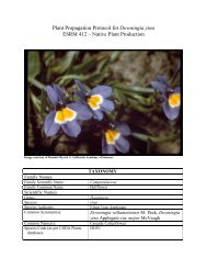
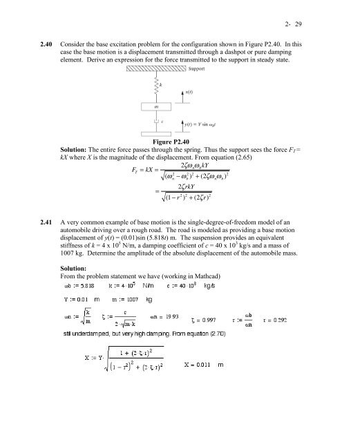
<strong>2.40</strong> <strong>Consider</strong> <strong>the</strong> <strong>base</strong> <strong>excitation</strong> <strong>problem</strong> <strong>for</strong> <strong>the</strong> configuration shown in Figure P<strong>2.40</strong>. In this<br />
case <strong>the</strong> <strong>base</strong> motion is a displacement transmitted through a dashpot or pure damping<br />
element. Derive an expression <strong>for</strong> <strong>the</strong> <strong>for</strong>ce transmitted to <strong>the</strong> support in steady state.<br />
Figure P<strong>2.40</strong><br />
Solution: The entire <strong>for</strong>ce passes through <strong>the</strong> spring. Thus <strong>the</strong> support sees <strong>the</strong> <strong>for</strong>ce FT =<br />
kX where X is <strong>the</strong> magnitude of <strong>the</strong> displacement. From equation (2.65)<br />
F T = kX =<br />
=<br />
2!" n" b kY<br />
2 2 2<br />
(" n # "b ) + (2!" n" b ) 2<br />
2!rkY<br />
(1# r 2 ) 2 + (2!r) 2<br />
2.41 A very common example of <strong>base</strong> motion is <strong>the</strong> single-degree-of-freedom model of an<br />
automobile driving over a rough road. The road is modeled as providing a <strong>base</strong> motion<br />
displacement of y(t) = (0.01)sin (5.818t) m. The suspension provides an equivalent<br />
stiffness of k = 4 x 10 5 N/m, a damping coefficient of c = 40 x 10 3 kg/s and a mass of<br />
1007 kg. Determine <strong>the</strong> amplitude of <strong>the</strong> absolute displacement of <strong>the</strong> automobile mass.<br />
Solution:<br />
From <strong>the</strong> <strong>problem</strong> statement we have (working in Mathcad)<br />
2-<br />
<strong>29</strong>
2.42 A vibrating mass of 300 kg, mounted on a massless support by a spring of stiffness<br />
40,000 N/m and a damper of unknown damping coefficient, is observed to vibrate with a<br />
10-mm amplitude while <strong>the</strong> support vibration has a maximum amplitude of only 2.5 mm<br />
(at resonance). Calculate <strong>the</strong> damping constant and <strong>the</strong> amplitude of <strong>the</strong> <strong>for</strong>ce on <strong>the</strong><br />
<strong>base</strong>.<br />
Solution:<br />
Given: m = 300 kg, k = 40,000 N/m, ! b = ! n (r = 1) , X = 10 mm, Y = 2.5 mm.<br />
Find damping constant (Equation 2.71)<br />
X<br />
Y =<br />
16 =<br />
c =<br />
1+ (2!r) 2<br />
(1" r 2 ) 2 + (2!r) 2<br />
#<br />
&<br />
%<br />
(<br />
$<br />
'<br />
1+ 4! 2<br />
4! 2<br />
4(40,000)(300)<br />
60<br />
1/ 2<br />
)<br />
10<br />
2.5<br />
" ! 2 = 1 c2<br />
=<br />
60 4km or<br />
= 894.4 kg/s<br />
Amplitude of <strong>for</strong>ce on <strong>base</strong>: (equation (2.76))<br />
F = kYr T 2 1+ (2!r) 2<br />
1" r 2 ( ) 2<br />
#<br />
%<br />
%<br />
$ %<br />
+ ( 2!r ) 2<br />
&<br />
(<br />
(<br />
'(<br />
1/ 2<br />
)<br />
"<br />
2<br />
1+ 4!<br />
=<br />
4! 2 $<br />
F = (40,000)(0.0025)(1) T 2<br />
1+ 4 1 * -<br />
+<br />
, 60.<br />
/<br />
4 1<br />
# &<br />
% (<br />
% (<br />
% * - (<br />
%<br />
+<br />
, 60.<br />
/ (<br />
$ '<br />
F = 400 N<br />
T<br />
#<br />
1/ 2<br />
)<br />
%<br />
'<br />
&<br />
1/ 2<br />
(<br />
2-<br />
30
Chapter Three Solutions<br />
Problem and Solutions <strong>for</strong> Section 3.1 (3.1 through 3.14)<br />
3.1 Calculate <strong>the</strong> solution to<br />
and plot <strong>the</strong> response.<br />
Solution: Given:<br />
! n =<br />
Total Solution:<br />
( )<br />
( ) = 1 !x ( 0)<br />
= 0<br />
!!x + 2 !x + 2x = ! t " #<br />
x 0<br />
!!x + 2 !x + 2x = ! ( t " # ) x( 0)<br />
= 1, !x ( 0)<br />
= 0<br />
k<br />
= 1.414 rad/s, " =<br />
m<br />
x t<br />
Homogeneous: From Equation (1.36)<br />
x t h ( ) = Ae !"# nt sin ( # t + $ d )<br />
( v + "# x 0 n 0 ) 2<br />
+ x # 0 d<br />
# d<br />
c<br />
2 km = 0.7071, ! d = ! n 1# " 2 = 1 rad/s<br />
( ) = x t h ( ) + x t p ( )<br />
( ) 2<br />
A =<br />
, $ = tan 2 !1 % x # (<br />
0 d<br />
' * = .785 rad<br />
& v + "# x 0 n 0 )<br />
+ x t h ( ) = 1.414e !t sin( t + .785)<br />
Particular: From Equation. (3.9)<br />
x t p ( ) = 1<br />
e<br />
m! d<br />
"#! n t "$ ( ) 1 t "%<br />
sin! t " $ d ( ) = e"<br />
( 1)<br />
( 1)<br />
( ) sin( t " % )<br />
" t "%<br />
But, sin ( "t)<br />
= "sint So, x t p ( ) = "e ( ) sint &<br />
x( t)<br />
= 1.414e !t sin( t + 0.785)<br />
0 < t < "<br />
x( t)<br />
= 1.414e !t sin( t + 0.785)<br />
! e !(t !" ) sint t > "<br />
This is plotted below using <strong>the</strong> Heaviside function.<br />
3- 1
3- 2
3.2 Calculate <strong>the</strong> solution to<br />
and plot <strong>the</strong> response.<br />
( )<br />
!!x + 2 !x + 3x = sint + ! t " #<br />
( ) = 0 !x ( 0)<br />
= 1<br />
x 0<br />
Solution: Given: !!x + 2 !x + 3x = sint + ! ( t " # ), x( 0)<br />
= 0, !x ( 0)<br />
= 0<br />
! = n<br />
k<br />
c<br />
= 1.732 rad/s, " =<br />
m 2 km = 0.5774, ! d = ! n 1# " 2 = 1.414 rad/s<br />
Total Solution:<br />
x t<br />
0 < t < !<br />
x t<br />
( ) = x h + x p1<br />
( ) = x h + x p1 + x p2 t > !<br />
Homogeneous: Eq. (1.36)<br />
xh t ( ) = Ae !"# nt sin ( # t + $ d ) = Ae !t sin 1.414t + $<br />
Particular: #1 (Chapter 2)<br />
( )<br />
( ), where ! = 1 rad/s . Note that f 0 = F 0<br />
x (t) = X sin !t " #<br />
p1 = 1<br />
m<br />
$ X =<br />
f0 2 2 ( ! " ! n ) 2<br />
+ ( 2%! ! n ) 2<br />
= 0.3536, and # = tan "1 2%! n ! & )<br />
( 2 2 +<br />
'(<br />
! " ! n * + = 0.785 rad<br />
$ x t p1( ) = 0.3536sin ( t " 0.7854)<br />
Particular: #2 Equation 3.9<br />
x t p2 ( ) = 1<br />
e "#! n t "$ ( ) sin! t " % d ( ) =<br />
1<br />
1<br />
t "$<br />
e" ( ) sin1.414( t " $ )<br />
m! d<br />
& x p2 t<br />
( ) = 0.7071e<br />
" t "$<br />
( ) ( 1.414)<br />
( )<br />
( ) sin1.414 t " $<br />
The total solution <strong>for</strong> 0< t
( ) = x h + x p1 + x p2<br />
3- 4<br />
x t<br />
x( t)<br />
= !0.433e !t ! t !"<br />
sin( 1.414t + 0.6155)<br />
+ 0.3536sin ( t ! 0.7854)<br />
! 0.7071e ( ) sin( 1.414t ! " ) t > "<br />
The response is plotted in <strong>the</strong> following (from Mathcad):<br />
3.3 Calculate <strong>the</strong> impulse response function <strong>for</strong> a critically damped system.<br />
Solution:<br />
The change in <strong>the</strong> velocity from an impulse isv0<br />
= ˆ F<br />
m , while x0 = 0. So <strong>for</strong> a critically<br />
damped system, we have from Eqs. 1.45 and 1.46 with x0 = 0:<br />
x(t) = v 0 te !" n t<br />
# x(t) = ˆF<br />
m te!" n t
3- 6<br />
3.6 <strong>Consider</strong> a simple model of an airplane wing given in Figure P3.6. The wing is<br />
approximated as vibrating back and <strong>for</strong>th in its plane, massless compared to <strong>the</strong> missile<br />
carriage system (of mass m). The modulus and <strong>the</strong> moment of inertia of <strong>the</strong> wing are<br />
approximated by E and I, respectively, and l is <strong>the</strong> length of <strong>the</strong> wing. The wing is<br />
modeled as a simple cantilever <strong>for</strong> <strong>the</strong> purpose of estimating <strong>the</strong> vibration resulting from<br />
<strong>the</strong> release of <strong>the</strong> missile, which is approximated by <strong>the</strong> impulse funciton Fδ(t).<br />
Calculate <strong>the</strong> response and plot your results <strong>for</strong> <strong>the</strong> case of an aluminum wing 2 m long<br />
with m = 1000 kg, ζ = 0.01, and I = 0.5 m 4 . Model F as 1000 N lasting over 10 -2 s.<br />
Modeling of wing vibration resulting from <strong>the</strong> release of a missile. (a) system of interest;<br />
(b) simplification of <strong>the</strong> detail of interest; (c) crude model of <strong>the</strong> wing: a cantilevered<br />
beam section (recall Figure 1.24); (d) vibration model used to calculate <strong>the</strong> response<br />
neglecting <strong>the</strong> mass of <strong>the</strong> wing.<br />
Solution: Given:<br />
m = 1000 kg ! = 0.01<br />
l = 4 m I = 0.5 m 4<br />
F = 1000 N "t = 10 -2 s<br />
From Table 1.2, <strong>the</strong> modulus of Aluminum is E = 7.1! 10 10 N/m 2<br />
The stiffness is<br />
( ) ( 0.5)<br />
k = 3EI<br />
! 3 = 3 7.1! 1010<br />
4 3<br />
" n =<br />
= 1.664 ! 10 9 N/m<br />
k<br />
m = 1.<strong>29</strong> ! 103 rad/s (205.4 Hz)<br />
" d = " n 1# $ 2 = 1.<strong>29</strong> ! 10 3
Solution (Eq. 3.6):<br />
( ) = F!t<br />
x t<br />
( )e "#$ n t<br />
m$ d<br />
sin$ t = 7.753 % 10 d "6 e "12.9t sin( 1<strong>29</strong>0t)<br />
m<br />
The following m-file<br />
t=(0:0.0001:0.5);<br />
F=1000;dt=0.01;m=1000;zeta=0.01;E=7.1*10^10;I=0.5;L=4;<br />
wn=sqrt((3*I*E/L^3)/m);<br />
wd=wn*sqrt(1-zeta^2);<br />
x=(F*dt/(m*wd))*exp(-zeta*wn*t).*sin(wd*t);<br />
plot(t,x)<br />
The solution worked out in Mathcad is given in <strong>the</strong> following:<br />
3- 7
3- 8
3- 18<br />
3.16 Calculate <strong>the</strong> response of an underdamped system to <strong>the</strong> <strong>excitation</strong> given in<br />
Figure P3.16.<br />
Plot of a pulse input of <strong>the</strong> <strong>for</strong>m f(t) = F 0sint.<br />
Solution:<br />
x( t)<br />
= F0 e<br />
m! d<br />
"#! nt $<br />
e "#! nt t<br />
x( t)<br />
= 1<br />
m! d<br />
F ( t)<br />
= F sin t 0<br />
)<br />
0<br />
Figure P3.16<br />
F ( $ )e #! n $ %<br />
&<br />
sin! t " $ d ( ) '<br />
( d$<br />
( ) t < * From Figure P3.16<br />
For t + *, x( t)<br />
= F0 m! d<br />
( )<br />
e "#! nt t<br />
)<br />
0<br />
sin$e #! n $ ( sin! t " $ d ( ) )d$<br />
1<br />
e<br />
2<br />
2 % 1+ 2! + ! '<br />
& d n (<br />
#! nt % ( ! " 1 d )sint " #! cost '<br />
&<br />
n ( " ! %<br />
)<br />
{ ( " 1 d )sin! t " #! cos! t<br />
d n d }<br />
)<br />
&<br />
1<br />
+<br />
e<br />
2<br />
2% 1+ 2! + ! '<br />
& d n (<br />
#! nt % ( ! " 1 d )sint " #! cost '<br />
&<br />
n ( + ! { ( " 1 d )sin! t " #! cos! t<br />
d n d } '<br />
*<br />
*<br />
(<br />
t<br />
For ! > ", : # f (! )h(t " ! )d! = # f (! )h(t " ! )d! + #<br />
(0)h(t " ! )d!<br />
0<br />
$<br />
0<br />
t<br />
$
x( t)<br />
= F0 m! d<br />
"<br />
0 1 +<br />
0<br />
* 2<br />
2" #<br />
1+ 2! + ! $<br />
d n<br />
#<br />
% ,+<br />
e "#! n t<br />
%<br />
&<br />
0<br />
sin$e #! n $ ( sin! t " $ d ( ) )d$<br />
= F0 e<br />
m! d<br />
"#! nt '<br />
e &! nt ) " ( ! ' 1 d )sin " ! t ' ( d<br />
#<br />
1 e<br />
+<br />
2<br />
2" 1+ 2! + ! $<br />
# d n %<br />
&! nt )<br />
+<br />
" ! + 1<br />
# d<br />
*<br />
,+<br />
( )<br />
( )<br />
$<br />
# % ' &! n cos ! " t ' ( $ $ -<br />
# d % % +<br />
.<br />
' ( ! ' 1 d )sin! t ' &! cos! t<br />
d n d /+<br />
( )sin " ! t ' 1 d<br />
( )<br />
( )<br />
3- 19<br />
$<br />
# % + &! cos ! " t ' ( $ $ -$<br />
# d % % +<br />
.<br />
2<br />
+ ( ! ' 1 d )sin! t ' &! cos! t<br />
2<br />
d n d /+<br />
%<br />
Alternately, one could take a Laplace Trans<strong>for</strong>m approach and assume <strong>the</strong> under-damped<br />
system is a mass-spring-damper system of <strong>the</strong> <strong>for</strong>m<br />
m!!x ( t)<br />
+ c!x ( t)<br />
+ kx( t)<br />
= F t<br />
The <strong>for</strong>cing function given can be written as<br />
F( t)<br />
= F0 ( H ( t)<br />
! H ( t ! " ) )sin t<br />
( )<br />
Normalizing <strong>the</strong> equation of motion yields<br />
!!x t ( ) + 2!" n !x t ( ) + " 2<br />
n x t<br />
where f 0 = F 0<br />
m<br />
( ) = f0 H t<br />
( ( ) # H ( t # $ ) )sin t<br />
and m, c and k are such that 0 < ! < 1.<br />
Assuming initial conditions, trans<strong>for</strong>ming <strong>the</strong> equation of motion into <strong>the</strong> Laplace domain<br />
yields<br />
X ( s)<br />
=<br />
!" s<br />
f0 ( 1+ e )<br />
2<br />
( )<br />
s 2 ( + 1)<br />
s 2 + 2#$ ns + $ n<br />
The above expression can be converted to partial fractions<br />
!" s ( )<br />
X ( s)<br />
= f0 1+ e<br />
#<br />
$<br />
%<br />
As + B<br />
s 2 + 1<br />
!" s ( )<br />
&<br />
'<br />
( + f0 1+ e<br />
where A, B, C, and D are found to be<br />
( )<br />
( )<br />
Cs + D<br />
s 2 #<br />
&<br />
2<br />
$<br />
% + 2)* ns + * n '<br />
(
A =<br />
B =<br />
C =<br />
!2"# n<br />
2 ( 1 ! # n ) 2<br />
+ 2"# n<br />
2 ( 1 ! # n ) 2<br />
2<br />
# n ! 1<br />
( ) 2<br />
+ ( 2"# n ) 2<br />
2"# n<br />
2 ( 1 ! # n ) 2<br />
+ 2"# n<br />
D = 1 ! # 2<br />
n<br />
2<br />
1! # n<br />
( ) 2<br />
( ) 2<br />
( ) 2<br />
( ) + 2"# n<br />
( ) 2<br />
+ 2"# n<br />
Notice that X ( s)<br />
can be written more attractively as<br />
X ( s)<br />
= f0 #<br />
$<br />
%<br />
= f 0 G s<br />
As + B<br />
s 2 + 1 +<br />
( ) + e )* s ( G( s)<br />
)<br />
Cs + D<br />
s 2 &<br />
2<br />
+ 2!" ns + " n '<br />
( + f0e )* s As + B<br />
%<br />
Per<strong>for</strong>ming <strong>the</strong> inverse Laplace Trans<strong>for</strong>m yields<br />
( ( ) )<br />
x( t)<br />
= f0 g( t)<br />
+ H ( t ! " )g t ! "<br />
where g(t) is given below<br />
g( t)<br />
= Acos( t)<br />
+ Bsin ( t)<br />
+ Ce !"# nt<br />
cos ( # dt ) + D ! C"# n<br />
%<br />
& # d<br />
! d is <strong>the</strong> damped natural frequency,! d = ! n 1" # 2 .<br />
$<br />
s 2 + 1 +<br />
Cs + D<br />
s 2 #<br />
&<br />
2<br />
$<br />
+ 2!" ns + " n '<br />
(<br />
'<br />
) e!"# nt sin # dt<br />
(<br />
( )<br />
3- 20<br />
Let m=1 kg, c=2 kg/sec, k=3 N/m, and F 0=2 N. The system is solved numerically. Both<br />
exact and numerical solutions are plotted below
Below is <strong>the</strong> code used to solve this <strong>problem</strong><br />
% Establish a time vector<br />
t=[0:0.001:10];<br />
Figure 1 Analytical vs. Numerical Solutions<br />
% Define <strong>the</strong> mass, spring stiffness and damping coefficient<br />
m=1;<br />
c=2;<br />
k=3;<br />
% Define <strong>the</strong> amplitude of <strong>the</strong> <strong>for</strong>cing function<br />
F0=2;<br />
% Calculate <strong>the</strong> natural frequency, damping ratio and normalized <strong>for</strong>ce amplitude<br />
zeta=c/(2*sqrt(k*m));<br />
wn=sqrt(k/m);<br />
f0=F0/m;<br />
% Calculate <strong>the</strong> damped natural frequency<br />
wd=wn*sqrt(1-zeta^2);<br />
% Below is <strong>the</strong> common denominator of A, B, C and D (partial fractions<br />
% coefficients)<br />
dummy=(1-wn^2)^2+(2*zeta*wn)^2;<br />
% Hence, A, B, C, and D are given by<br />
A=-2*zeta*wn/dummy;<br />
B=(wn^2-1)/dummy;<br />
C=2*zeta*wn/dummy;<br />
3- 21
D=((1-wn^2)+(2*zeta*wn)^2)/dummy;<br />
3- 22<br />
% EXACT SOLUTION<br />
%<br />
************************************************************************<br />
*<br />
%<br />
************************************************************************<br />
*<br />
<strong>for</strong> i=1:length(t)<br />
% Start by defining <strong>the</strong> function g(t)<br />
g(i)=A*cos(t(i))+B*sin(t(i))+C*exp(-zeta*wn*t(i))*cos(wd*t(i))+((D-<br />
C*zeta*wn)/wd)*exp(-zeta*wn*t(i))*sin(wd*t(i));<br />
% Be<strong>for</strong>e t=pi, <strong>the</strong> response will be only g(t)<br />
if t(i)
% s^2+2*zeta*wn+wn^2<br />
% Define <strong>the</strong> numerator and denominator<br />
num=[1];<br />
den=[1 2*zeta*wn wn^2];<br />
% Establish <strong>the</strong> transfer function<br />
sys=tf(num,den);<br />
% Obtain <strong>the</strong> solution using lsim<br />
xn=lsim(sys,f,t);<br />
% Plot <strong>the</strong> results<br />
figure;<br />
set(gcf,'Color','White');<br />
plot(t,xe,t,xn,'--');<br />
xlabel('Time(sec)');<br />
ylabel('Response');<br />
legend('Forcing Function','Exact Solution','Numerical Solution');<br />
text(6,0.05,'\uparrow','FontSize',18);<br />
axes('Position',[0.55 0.3/0.8 0.25 0.25])<br />
plot(t(6001:6030),xe(6001:6030),t(6001:6030),xn(6001:6030),'--');<br />
3- 23<br />
3.17 Speed bumps are used to <strong>for</strong>ce drivers to slow down. Figure P3.17 is a model of a<br />
car going over a speed bump. Using <strong>the</strong> data from Example 2.4.1 and an<br />
undamped model of <strong>the</strong> suspension system (k = 4 x 10 5 N/m, m = 1007 kg), find<br />
an expression <strong>for</strong> <strong>the</strong> maximum relative deflection of <strong>the</strong> car’s mass versus <strong>the</strong><br />
velocity of <strong>the</strong> car. Model <strong>the</strong> bump as a half sine of length 40 cm and height 20<br />
cm. Note that this is a moving <strong>base</strong> <strong>problem</strong>.
3.22 <strong>Consider</strong> <strong>the</strong> step response described in Figure 3.7. Calculate t p by noting that it<br />
occurs at <strong>the</strong> first peak, or critical point, of <strong>the</strong> curve.<br />
Solution: Assume t 0 = 0. The response is given by Eq. (3.17):<br />
x( t)<br />
= F0 k !<br />
F 0<br />
k 1! " 2<br />
To find t p, compute <strong>the</strong> derivative and let<br />
!x ( t)<br />
=<br />
!F 0<br />
k 1! " 2<br />
!"# e n !"# nt %<br />
&<br />
cos # t ! $ d<br />
e !"# nt cos ( # t ! $ d )<br />
!x ( t)<br />
= 0<br />
) !"# cos # n ( t ! $ d ) ! # sin # t ! $<br />
d d<br />
( ) + e !"# nt ( !# d )sin # t ! $ d<br />
( ) = 0<br />
( )<br />
'<br />
( = 0<br />
3- 32<br />
) tan ( # t ! $ d ) = !"# n<br />
# d<br />
! t " # " $ = tan d "1 "%! & )<br />
n<br />
(<br />
' !<br />
+<br />
d *<br />
(π can be added or subtracted without changing <strong>the</strong><br />
tangent of an angle)<br />
t = 1<br />
" + # + tan<br />
! d<br />
$1 $%! ,<br />
& ) /<br />
n<br />
.<br />
(<br />
' !<br />
+ 1<br />
-.<br />
d * 01<br />
But, ! = tan "1<br />
$<br />
&<br />
%<br />
&<br />
So,<br />
#<br />
1" # 2<br />
'<br />
)<br />
(<br />
)<br />
t = 1<br />
" + tan<br />
! d<br />
#1<br />
+ %<br />
- '<br />
- &<br />
'<br />
,<br />
t = p "<br />
! d<br />
$<br />
1# $ 2<br />
(<br />
*<br />
)<br />
* # tan#1<br />
% $<br />
'<br />
&<br />
'<br />
1# $ 2<br />
( .<br />
* 0<br />
)<br />
* 0<br />
/
3.23 Calculate <strong>the</strong> value of <strong>the</strong> overshoot (o.s.), <strong>for</strong> <strong>the</strong> system of Figure P3.7.<br />
Solution:<br />
The overshoot occurs at t = p !<br />
" d<br />
Substitute into Eq. (3.17):<br />
The overshoot is<br />
Since ! = tan "1<br />
$<br />
&<br />
%<br />
&<br />
( ) = F 0<br />
x t p<br />
k !<br />
F0 k 1! " 2<br />
e !"# n $ /# d cos . # d<br />
.<br />
o.s. = x( t p ) ! x t ss ( )<br />
o.s. = F 0<br />
k !<br />
#<br />
1" # 2<br />
F 0<br />
k 1! " 2<br />
'<br />
)<br />
(<br />
) , <strong>the</strong>n cos! = 1-# 2<br />
o.s. = !<br />
F 0<br />
k 1! " 2<br />
,<br />
-<br />
% $ (<br />
'<br />
& #<br />
*<br />
d )<br />
! +<br />
/<br />
1<br />
01<br />
e !"# n $ /# d ( !cos% ) ! F0 k<br />
e !"# n $ /# d ( ) 1! " 2 ( )<br />
o.s. = F 0<br />
k e!"# n $ /# d<br />
3.24 It is desired to design a system so that its step response has a settling time of 3 s<br />
and a time to peak of 1 s. Calculate <strong>the</strong> appropriate natural frequency and<br />
damping ratio to use in <strong>the</strong> design.<br />
Solution:<br />
Given ts = 3s, t = 1s p<br />
Settling time:<br />
Peak time:<br />
t p = !<br />
" d<br />
t s = 3.5<br />
!" n<br />
= 3 s #!" n = 3.5<br />
3<br />
= 1.1667 rad/s<br />
= 1 s # " d = " n 1$ % 2 = ! rad/s<br />
# " 1$ n 1.1667 & )<br />
( +<br />
' *<br />
# " n<br />
" n<br />
, 2 1.3611/<br />
. 1$ 2 1<br />
-.<br />
" n 0<br />
2<br />
= ! # " n<br />
, & 2 1.1667)<br />
. 1$<br />
.<br />
(<br />
' "<br />
+<br />
n *<br />
-<br />
2<br />
/<br />
1<br />
1<br />
0<br />
= ! 2<br />
1 = ! 2 2 2<br />
# " $ 1.311 = ! # " = 3.35 rad/s<br />
n<br />
n<br />
3- 33
Problems and Solutions <strong>for</strong> Section 3.7 (3.45 through 3.52)<br />
3.45 Using complex algebra, derive equation (3.89) from (3.86) with s = jω.<br />
Solution: From equation (3.86):<br />
Substituting s = j! yields<br />
H ( j! ) =<br />
The magnitude is given by<br />
H ( j! dr ) =<br />
) "<br />
+ $<br />
+<br />
#<br />
$<br />
* +<br />
H ( j! ) =<br />
H ( s)<br />
=<br />
1<br />
m( j! ) 2<br />
+ c j!<br />
1<br />
1<br />
ms 2 + cs + k<br />
( ) + k<br />
m( j! ) 2<br />
+ ( cj! ) + k<br />
1<br />
k " m! 2 ( ) 2<br />
+ ( c! ) 2<br />
1<br />
=<br />
k " m! 2 " cj!<br />
%<br />
'<br />
&<br />
' =<br />
1<br />
k ( m! 2 "<br />
%<br />
,<br />
.<br />
$<br />
'<br />
# ( cj! & .<br />
-.<br />
which is Eq. (3.89)<br />
1/ 2<br />
3- 61<br />
3.46 Using <strong>the</strong> plot in Figure 3.20, estimate <strong>the</strong> system’s parameters m, c, and k, as well as <strong>the</strong><br />
natural frequency.<br />
Solution: From Fig. 3.20<br />
1<br />
k<br />
= 2 ! k = 0.5<br />
k<br />
" = " = 0.25 = ! m = 8<br />
n<br />
m<br />
1<br />
# 4.6 ! c = 0.087<br />
c"
3- 67<br />
3.52 An experimental (compliance) magnitude plot is illustrated in Fig. P3.52. Determine<br />
!,",c,m, and k. Assume that <strong>the</strong> units correspond to m/N along <strong>the</strong> vertical axis.<br />
Solution: Referring to <strong>the</strong> plot, it starts at<br />
1<br />
H(! j) =<br />
k<br />
1<br />
Thus:<br />
0.05 = ! k = 20 N/m<br />
k<br />
At <strong>the</strong> peak, ωn = ω = 3 rad/s. Thus <strong>the</strong> mass can be determined by<br />
m = k<br />
2<br />
! n<br />
" m = 2.22 kg<br />
The damping is found from<br />
1<br />
c<br />
= 0.11 " c = 3.03 kg/s " # =<br />
c! 2 km =<br />
3.03<br />
= 0.227<br />
2 20 $ 2.22
AA-312 Homework # 3 (Solutions)<br />
Problem A<br />
Let a = −1 + i5, b = 6 + i3 and c = −2 − i4,<br />
1. Express <strong>the</strong> complex variables a, b and c in <strong>the</strong> <strong>for</strong>m<br />
a = -1.0000 + 5.0000i<br />
b = 6.0000 + 3.0000i<br />
c = -2.0000 - 4.0000i<br />
abs(a) = 5.0990<br />
angle(a) = 1.7682<br />
abs(b) = 6.7082<br />
angle(b) = 0.4636<br />
abs(c) = 4.4721<br />
angle(c) = -2.0344<br />
a = 5.0990e i1.7682<br />
b = 6.7082e i0.4636<br />
c = 4.4721e −i2.0344<br />
2. Find <strong>the</strong> product z = a ∗ b ∗ c. Show that z is equal to AaAbAce i(θa+θb+θc) .<br />
and<br />
z = 150 + i30 = 152.9706e i0.1974<br />
AaAbAc = 5.0990 ∗ 6.7082 ∗ 4.4721 = 152.9706<br />
θa + θb + θc = 1.7682 + 0.4636 + −2.0344 = 0.1974<br />
3. Find <strong>the</strong> ratio r = a/b. Show that r is equal to Aa<br />
Ab ei(θa−θb)<br />
and<br />
r = 0.2000 + i0.7333 = 0.7601e i1.3045<br />
Aa<br />
Ab<br />
= 5.0990<br />
6.7082<br />
= 0.7601<br />
θa − θb = 1.7682 − 0.4636 = 1.3045<br />
1
2 Uy-Loi Ly<br />
x(t)<br />
Problem B<br />
Let<br />
0.18<br />
0.16<br />
0.14<br />
0.12<br />
0.1<br />
0.08<br />
0.06<br />
0.04<br />
0.02<br />
0<br />
0 2 4 6 8 10<br />
Time (sec)<br />
Figure 1: Problem B<br />
X(s) =<br />
Fo<br />
s (ms 2 + cs + k)<br />
where Fo = 100 N, m = 10 kg, c = 10 N-sec/m and k = 1000 N/m. Find <strong>the</strong> response x(t).<br />
What is <strong>the</strong> steady-state response of x(t)?<br />
X(s) =<br />
100<br />
s(10s 2 + 10s + 1000)<br />
s + 1<br />
= −<br />
10s2 + 10s + 1000<br />
X(s) = − 0.1[(s + 0.5) + 0.5/√ 9.75 ∗ √ 9.75]<br />
(s + 0.5) 2 + 9.75<br />
+ 0.1<br />
s<br />
+ 0.1<br />
s<br />
Taking <strong>the</strong> inverse Laplace trans<strong>for</strong>m,<br />
x(t) = −0.1e −0.5t<br />
�<br />
cos √ 9.75t + 0.5<br />
√ sin<br />
9.75 √ �<br />
9.75t + 0.1<br />
The steady-state response is xss(t) = 0.1. Response x(t) is shown in Figure 1.