1 Precision alignment of the LIGO 4 km arms using ... - LIGO - Caltech
1 Precision alignment of the LIGO 4 km arms using ... - LIGO - Caltech
1 Precision alignment of the LIGO 4 km arms using ... - LIGO - Caltech

Create successful ePaper yourself
Turn your PDF publications into a flip-book with our unique Google optimized e-Paper software.
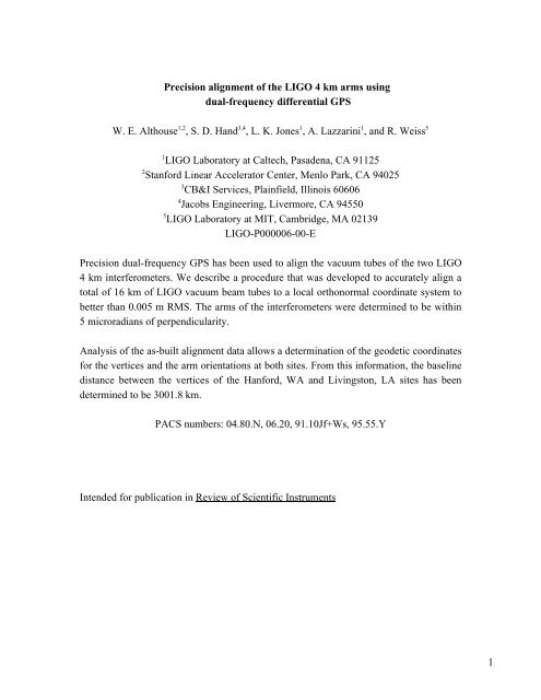
<strong>Precision</strong> <strong>alignment</strong> <strong>of</strong> <strong>the</strong> <strong>LIGO</strong> 4 <strong>km</strong> <strong>arms</strong> <strong>using</strong><br />
dual-frequency differential GPS<br />
W. E. Althouse 1,2 , S. D. Hand 3,4 , L. K. Jones 1 , A. Lazzarini 1 , and R. Weiss 5<br />
1 <strong>LIGO</strong> Laboratory at <strong>Caltech</strong>, Pasadena, CA 91125<br />
2 Stanford Linear Accelerator Center, Menlo Park, CA 94025<br />
3 CB&I Services, Plainfield, Illinois 60606<br />
4 Jacobs Engineering, Livermore, CA 94550<br />
5 <strong>LIGO</strong> Laboratory at MIT, Cambridge, MA 02139<br />
<strong>LIGO</strong>-P000006-00-E<br />
<strong>Precision</strong> dual-frequency GPS has been used to align <strong>the</strong> vacuum tubes <strong>of</strong> <strong>the</strong> two <strong>LIGO</strong><br />
4 <strong>km</strong> interferometers. We describe a procedure that was developed to accurately align a<br />
total <strong>of</strong> 16 <strong>km</strong> <strong>of</strong> <strong>LIGO</strong> vacuum beam tubes to a local orthonormal coordinate system to<br />
better than 0.005 m RMS. The <strong>arms</strong> <strong>of</strong> <strong>the</strong> interferometers were determined to be within<br />
5 microradians <strong>of</strong> perpendicularity.<br />
Analysis <strong>of</strong> <strong>the</strong> as-built <strong>alignment</strong> data allows a determination <strong>of</strong> <strong>the</strong> geodetic coordinates<br />
for <strong>the</strong> vertices and <strong>the</strong> arm orientations at both sites. From this information, <strong>the</strong> baseline<br />
distance between <strong>the</strong> vertices <strong>of</strong> <strong>the</strong> Hanford, WA and Livingston, LA sites has been<br />
determined to be 3001.8 <strong>km</strong>.<br />
PACS numbers: 04.80.N, 06.20, 91.10Jf+Ws, 95.55.Y<br />
Intended for publication in Review <strong>of</strong> Scientific Instruments<br />
1
I. Introduction<br />
The Laser Interferometer Gravitational-wave Observatory (<strong>LIGO</strong>) 1,2,3 is dedicated to <strong>the</strong><br />
direct measurement <strong>of</strong> gravitational waves from astrophysical sources. The project is<br />
funded by <strong>the</strong> National Science Foundation and is operated jointly by <strong>the</strong> California<br />
Institute <strong>of</strong> Technology (<strong>Caltech</strong>) and <strong>the</strong> Massachusetts Institute <strong>of</strong> Technology (MIT).<br />
Gravitational waves are emitted by accelerating masses and are expected to be detectable<br />
at <strong>the</strong> Earth from sufficiently violent events occurring throughout <strong>the</strong> universe 4 . The<br />
formation and collision <strong>of</strong> black holes and <strong>the</strong> coalescence <strong>of</strong> orbiting compact stars, such<br />
as binary neutron stars or black holes, are likely sources. In addition, <strong>the</strong>re is a possible<br />
residue from <strong>the</strong> primeval universal explosion. Einstein's Theory <strong>of</strong> General Relativity<br />
predicts that <strong>the</strong> waves travel at <strong>the</strong> speed <strong>of</strong> light and that <strong>the</strong>y cause a distortion <strong>of</strong><br />
spacetime transverse to <strong>the</strong>ir direction <strong>of</strong> propagation 5,6 .<br />
The direct detection <strong>of</strong> gravitational waves can provide fundamental evidence for <strong>the</strong><br />
behavior <strong>of</strong> spacetime in strong gravitational fields where Newtonian gravitation is no<br />
longer a good approximation. Detection may also yield a new view <strong>of</strong> <strong>the</strong> universe since<br />
gravitational waves emerge from <strong>the</strong> densest regions in astrophysical processes without<br />
attenuation or scattering.<br />
<strong>LIGO</strong> detects <strong>the</strong> gravitational waves by comparing <strong>the</strong> time <strong>of</strong> propagation <strong>of</strong> light in<br />
mutually orthogonal paths in <strong>the</strong> distorted space between freely suspended test masses<br />
separated by 4 <strong>km</strong> <strong>using</strong> laser interferometry 7 . The distortions that need to be measured<br />
are not expected to be larger than a strain <strong>of</strong> 10 -21 . The tubes, aligned by <strong>the</strong> GPS system<br />
described here, provide an evacuated and low scattering path for <strong>the</strong> laser beams (see<br />
Figure 1).<br />
The <strong>LIGO</strong> facilities consist <strong>of</strong> two observatories, one located at <strong>the</strong> DOE Hanford<br />
Nuclear Reservation in Washington State (<strong>LIGO</strong> Hanford Observatory or LHO, see<br />
Figure 2) and <strong>the</strong> o<strong>the</strong>r in Livingston Parish, Louisiana (<strong>LIGO</strong> Livingston Observatory or<br />
LLO). The site-to-site separation is 3002 <strong>km</strong>. This distance corresponds to a gravitational<br />
wave travel time <strong>of</strong> 10 ms. The interferometers located at <strong>the</strong> two sites are operated as a<br />
network. A network <strong>of</strong> detectors enables <strong>the</strong> determination <strong>of</strong> <strong>the</strong> position <strong>of</strong> sources on<br />
<strong>the</strong> sky from arrival time differences <strong>of</strong> <strong>the</strong> wave. It also reduces <strong>the</strong> influence <strong>of</strong> non-<br />
Gaussian environmental noise in <strong>the</strong> individual interferometers and <strong>the</strong>reby increases<br />
detection confidence.<br />
2
II. Method <strong>of</strong> <strong>alignment</strong><br />
CB&I Services, Inc. (CB&I), was contracted by <strong>LIGO</strong> to design, fabricate, install and<br />
align <strong>the</strong> beam tubes. A major concern for <strong>LIGO</strong> was <strong>alignment</strong> <strong>of</strong> <strong>the</strong> 4 <strong>km</strong> beam tubes.<br />
The tubes must have a minimum clear aperture <strong>of</strong> 1 m to accommodate multiple<br />
interferometers operating simultaneously within <strong>the</strong> same vacuum envelope and to<br />
maintain tube scattering and diffraction at an acceptable level for <strong>the</strong> most sensitive<br />
detectors contemplated in <strong>the</strong> facilities. Refer to Figure 3.<br />
The beam tubes are fabricated from 3 mm thick spirally welded 304L stainless steel and<br />
have a nominal aperture diameter <strong>of</strong> 1.24 meters. 9 cm high optical baffles installed in <strong>the</strong><br />
beam tube reduce <strong>the</strong> nominal aperture to 1 m. The difference between <strong>the</strong> required clear<br />
aperture (1 m) and <strong>the</strong> nominal aperture is accounted for by a number <strong>of</strong> design and<br />
fabrication details. These are discussed below. Construction <strong>of</strong> <strong>the</strong> beam tubes was<br />
undertaken in 2 <strong>km</strong> sections, called beam tube modules.<br />
A. Feasibility studies and design<br />
<strong>LIGO</strong> had identified in its 1989 conceptual design 8 <strong>the</strong> use <strong>of</strong> a high precision dualfrequency,<br />
differential Global Positioning System survey (GPS or DGPS) as a technique<br />
to set reference monuments that could be used as millimeter-level optical benchmarks.<br />
However, at <strong>the</strong> time <strong>of</strong> <strong>the</strong> proposal, GPS equipment and procedures were not yet<br />
commercially available.<br />
The introduction <strong>of</strong> commercially available, real time DGPS systems in 1993 permitted<br />
<strong>the</strong> use <strong>of</strong> GPS to be reconsidered by <strong>the</strong> time construction <strong>of</strong> <strong>the</strong> beam tube was to begin.<br />
Trimble Navigation's Site Surveyor Real Time Kinematic (RTK) system was identified as<br />
an <strong>of</strong>f-<strong>the</strong>-shelf system with millimeter-level accuracy that could perform in real time as<br />
needed in <strong>the</strong> field.<br />
A field demonstration was performed to evaluate <strong>the</strong> capability <strong>of</strong> accurately measuring<br />
millimeter displacements <strong>using</strong> <strong>the</strong> dual frequency system. This test was performed by<br />
displacing a GPS receiver antenna vertically and horizontally with a translation stage and<br />
<strong>the</strong>n comparing <strong>the</strong> GPS readout to a mechanical dial indicator. Accuracy and precision<br />
tests were performed with an integration time <strong>of</strong> 10 s. A total <strong>of</strong> ~260 points were<br />
measured for each <strong>of</strong> 3 displacement directions. Post-processing <strong>using</strong> a precise satellite<br />
ephemeris yielded 1σ (1-axis, horizontal) = 0.0009 m and 1σ (1-axis, vertical) = 0.0025<br />
m (see Figure 4). The data also exhibited biases (i.e., non-zeroes means or <strong>of</strong>fsets) in <strong>the</strong><br />
distribution <strong>of</strong> residuals. The horizontal performance conforms very well to a normally<br />
3
distributed set <strong>of</strong> measurements. However, <strong>the</strong> vertical data exhibit a bimodality which in<br />
<strong>the</strong> raw measurement-versus-actual displacement data sets resembles a nonlinearity for<br />
small vertical displacements. This may have come from <strong>the</strong> linear translation stage which<br />
was employed. As a conservative estimate <strong>of</strong> overall measurement uncertainty, <strong>the</strong> root<br />
sum square (RSS) <strong>of</strong> measurement bias and variance was used for both axes. These<br />
results were used in <strong>the</strong> χ 2 analysis described later.<br />
Similar repeatability tests were later conducted for each arm at both sites to confirm that<br />
no systematic effects were present. This also demonstrated that millimeter RMS precision<br />
was achievable along <strong>the</strong> 4 <strong>km</strong> <strong>arms</strong>.<br />
The early field test results were incorporated in <strong>the</strong> final design <strong>of</strong> <strong>the</strong> beam tube. The<br />
nominal beam tube diameter was chosen as a trade between (i) material costs, (ii)<br />
dimensional control <strong>of</strong> <strong>the</strong> fabrication process and (iii) beam tube <strong>alignment</strong> accuracy.<br />
The trade study resulted in <strong>the</strong> allocation <strong>of</strong> errors presented in Table 1.<br />
The beam tube supports were designed to incorporate a heavy stiffener with precision<br />
machined inside and outside surfaces to provide a center reference. By incorporating tight<br />
tolerances for concentricity <strong>of</strong> <strong>the</strong> stiffener rings, <strong>the</strong>ir outside diameter could be used as<br />
a reference to <strong>the</strong> beam tube centerline.<br />
B. GPS equipment<br />
CB&I chose Trimble Navigation’s Site Surveyor System for use on this project 9 . The<br />
following hardware configuration was used:<br />
• GPS Dual Frequency Receivers 4000SSi with OTF and lMB Memory<br />
• Data Collector TDC-1<br />
• Geodetic Ground Plane Antennas<br />
• Trim Talk Radio System<br />
• GPSurvey S<strong>of</strong>tware<br />
• TrimMap S<strong>of</strong>tware<br />
• Pacific Crest 35 W radio system in lieu <strong>of</strong> <strong>the</strong> Trimtalk Systems<br />
• 38 cm (15") Dorn-Margolan Choke Ring antennas to replace <strong>the</strong> Geodetic Ground<br />
Plane Antennas.<br />
The 1MB RAM in <strong>the</strong> receiver was insufficient to accommodate a full day <strong>of</strong> acquired<br />
data at <strong>the</strong> 5 s integration and sampling rate that was used. The field technician was<br />
required to halt data acquisition and to download <strong>the</strong> fixed and roving receiver databases<br />
4
at 4-hour intervals. A minimum <strong>of</strong> 3MB would have greatly improved operational<br />
efficiency in <strong>the</strong> field.<br />
C. Field implementation<br />
1. Layout <strong>of</strong> <strong>the</strong> global coordinate system<br />
The fundamental coordinate system for <strong>the</strong> <strong>alignment</strong> was <strong>the</strong> Earth ellipsoidal model<br />
WGS-84 10,11 . All raw GPS data were referred to this system <strong>using</strong> geodetic coordinates<br />
{height above ellipsoid [h], latitude [φ], longitude [λ]}. Geodetic coordinates were<br />
transformed to <strong>the</strong> standard earth-fixed Cartesian system {X E , Y E , Z E }, where z ˆ E is<br />
aligned along <strong>the</strong> earth’s polar axis and ˆ x E penetrates <strong>the</strong> ellipsoid at <strong>the</strong> intersection <strong>of</strong><br />
<strong>the</strong> Greenwich Meridian with <strong>the</strong> Equator. ˆ y E is perpendicular to both axes (refer to<br />
APPENDIX A).<br />
A global coordinate system (denoted by a subscript "G") specific to each <strong>LIGO</strong> site was<br />
defined in which <strong>the</strong> x ˆ G and y ˆ G are aligned along <strong>the</strong> interferometer <strong>arms</strong> and z ˆ G is<br />
normal to <strong>the</strong>se axes. The interferometer plane was chosen to minimize construction costs<br />
(determined by <strong>the</strong> local topography) such that <strong>the</strong> global coordinate system lies in a<br />
plane that is locally tangent to <strong>the</strong> WGS-84 model at some point within <strong>the</strong> triangle<br />
defined by <strong>the</strong> 4 <strong>km</strong> <strong>arms</strong>. Deviations between local Zenith and ˆ z G can range up to ~0.63<br />
× 10 -3 radian. The global coordinate systems for <strong>the</strong> two sites are fur<strong>the</strong>r described in data<br />
analysis discussion in Section III.<br />
The ends <strong>of</strong> <strong>the</strong> beam tube modules along each arm (i.e., at ~46 m, ~2012 m, ~2022 m, ~<br />
3989 m from <strong>the</strong> vertex) constituted controlled interface points. These points were<br />
identified by benchmarks (monuments) having measured geodetic coordinates that were<br />
provided by an independent surveyor. CB&I used <strong>the</strong>se points toge<strong>the</strong>r with an array <strong>of</strong><br />
five o<strong>the</strong>r <strong>LIGO</strong> primary GPS monuments to calibrate <strong>the</strong>ir GPS instrumentation and<br />
s<strong>of</strong>tware. The installation and survey <strong>of</strong> primary monuments was performed prior to<br />
beginning <strong>of</strong> <strong>the</strong> construction activities at <strong>the</strong> sites. At LHO <strong>the</strong> work was performed by<br />
<strong>the</strong> state Department <strong>of</strong> Transportation (WADOT) and it was performed by a private<br />
surveyor at LLO. The calibration was used by <strong>the</strong> GPS data acquisition system in real<br />
time to provide <strong>alignment</strong> data in global coordinates.<br />
5
Using global coordinates, <strong>the</strong> beam tube centerlines were marked along <strong>the</strong> foundation<br />
slab at points spaced uniformly at ~20 m intervals (<strong>the</strong> unit length <strong>of</strong> beam tube sections<br />
that were welded toge<strong>the</strong>r in <strong>the</strong> field) along both <strong>arms</strong>.<br />
A straight line in space varies in ellipsoidal height by ~1.25 m over a 4 <strong>km</strong> baseline. At<br />
each <strong>of</strong> <strong>the</strong> fiducial points, <strong>the</strong> design ellipsoidal height <strong>of</strong> <strong>the</strong> beam tube centerline was<br />
calculated <strong>using</strong> <strong>the</strong> WGS-84 model with <strong>the</strong> latitude and longitude as inputs. These<br />
heights were used to perform preliminary <strong>alignment</strong> <strong>of</strong> <strong>the</strong> tube sections as <strong>the</strong> supports<br />
were installed during beam tube fabrication on <strong>the</strong> slab.<br />
Fiducial points were surveyed <strong>using</strong> a layout cart (refer to Figure 5). The cart was<br />
equipped with linear bearings and a plumb <strong>alignment</strong> bracket and modified to support a<br />
fixed height antenna rod. Antenna rods, levels and attachment fixtures were periodically<br />
calibrated to better than 0.25 mm accuracy to ensure repeatability <strong>of</strong> measurements.<br />
Antenna rods used a leveling device consisting <strong>of</strong> a coincidence-type bubble level with a<br />
sensitivity <strong>of</strong> 10 arcsec/mm. This arrangement provided acceptable repeatability in a<br />
reasonable set-up time. After a nominal fiducial point was identified, a 15 - 20 minute<br />
static control point measurement was taken to provide a location determination. The<br />
nominal fiducial point was adjusted if required and a scribed mark was made on <strong>the</strong><br />
foundation slab for <strong>the</strong> tube installation crew to use for rough elevation and centering <strong>of</strong><br />
<strong>the</strong> tube section and its support.<br />
2. Final Alignment<br />
At Hanford, supports were aligned for <strong>the</strong> final time after installation had proceeded 3 - 4<br />
sections, i.e. ~80 m from <strong>the</strong> installation activity. This was just before <strong>the</strong> beam tube<br />
became covered by cement enclosures and was thus no longer directly available. At<br />
Livingston, <strong>the</strong> beam tube enclosure sections were core drilled directly over <strong>the</strong> beam<br />
tube supports at ~120 m intervals. This design improvement allowed <strong>alignment</strong> to be<br />
confirmed after fabrication was completed.<br />
The final <strong>alignment</strong> fixtures were similar for both sites (refer to Figure 6). The antenna<br />
rod was longer in Livingston to enable <strong>the</strong> antenna to protrude through <strong>the</strong> cored<br />
enclosure. The fixture was a high accuracy centering head clamped on <strong>the</strong> machined<br />
beam tube support stiffener ring, plumbed <strong>using</strong> a coincidence level and centered relative<br />
to <strong>the</strong> beam tube support stiffening ring. The GPS antenna 12 was attached to a rod <strong>of</strong><br />
calibrated length. The reference distance from <strong>the</strong> beam tube centerline to <strong>the</strong> antenna<br />
was taken as <strong>the</strong> rod length plus <strong>the</strong> radius <strong>of</strong> <strong>the</strong> beam tube support stiffener.<br />
6
With this fixture in place, <strong>the</strong> GPS receiver was set to <strong>the</strong> RTK "stake-out" mode to<br />
position <strong>the</strong> beam tube center to <strong>the</strong> desired position relative to <strong>the</strong> global coordinate<br />
system. Once <strong>the</strong> position was determined to be within a few mm <strong>of</strong> <strong>the</strong> desired location,<br />
<strong>the</strong> support was locked down. A 30 minute control point measurement was <strong>the</strong>n taken<br />
and <strong>the</strong> raw data were logged by <strong>the</strong> receiver for subsequent post processing. The control<br />
measurement was taken in <strong>the</strong> RTK mode to verify position and to allow real-time<br />
adjustment. Whenever an adjustment was required, a repeat 30 minute control<br />
measurement was taken to verify <strong>the</strong> change.<br />
3. GPS reference points outside enclosures<br />
Additional GPS reference points were located (only at LHO) outside <strong>the</strong> beam tube<br />
covers to provide <strong>the</strong> ability to monitor <strong>the</strong> foundation slab for long-term height changes<br />
from settlement. These reference points were placed at <strong>the</strong> edge <strong>of</strong> <strong>the</strong> foundation slab in<br />
line with each support ring. A two axis centering tripod designed to hold and adjust a<br />
fixed length GPS antenna rod was used (refer to Figure 7). A 30 minute static control<br />
point measurement was taken for each point. In addition, a cross-check was made <strong>using</strong><br />
Trimble’s RTK stake-out procedure. These data serve as a reference for future GPS<br />
surveys that are made to assess slab settlement.<br />
4. Post processing and data review in <strong>the</strong> field<br />
Data quality review was incorporated as part <strong>the</strong> daily field <strong>alignment</strong> procedure. Precise<br />
GPS satellite ephemeris data were employed to determine post-processed positions. The<br />
ephemeris data were downloaded from <strong>the</strong> US Coast Guard web site 13 .<br />
Satellite residuals for each data point were determined relative to <strong>the</strong> reference mean for<br />
that point. Residuals were evaluated for consistency with <strong>the</strong> mean to identify and<br />
eliminate outliers. For every point surveyed, <strong>the</strong> time dependence <strong>of</strong> residuals from all<br />
visible satellites were displayed graphically. Typically, outliers arise from data coming<br />
from satellites lying closest to <strong>the</strong> local horizon. Residuals exhibiting non-statistical<br />
fluctuations were eliminated by moving <strong>the</strong> satellite elevation cut<strong>of</strong>f to higher zenith<br />
angles or by eliminating data from suspect satellites. There is a trade-<strong>of</strong>f between<br />
degradation <strong>of</strong> signal-to-noise ratio (SNR), which decreases as satellites are removed<br />
from <strong>the</strong> analysis, and better data repeatability, which improves as data from marginally<br />
visible satellites are removed. After post processing, CB&I determined <strong>the</strong> geodetic<br />
coordinates <strong>of</strong> all points measured along <strong>the</strong> beam tubes. These were provided to <strong>LIGO</strong><br />
for fur<strong>the</strong>r analysis.<br />
7
III. Definition <strong>of</strong> global coordinate systems and analysis <strong>of</strong> beam tube <strong>alignment</strong><br />
data<br />
The as-built <strong>alignment</strong> data provided by CB&I were analyzed by <strong>LIGO</strong> to determine <strong>the</strong><br />
residuals relative to <strong>the</strong> best-fit descriptions for each site <strong>of</strong> <strong>the</strong> local right-handed<br />
coordinate systems that have <strong>the</strong>ir X and Y axes aligned along <strong>the</strong> beam tube <strong>arms</strong>. The<br />
methods employed at each site differed and reflected <strong>the</strong> accrued experience. These are<br />
described below.<br />
A. Hanford, Washington<br />
1. Definition <strong>of</strong> <strong>the</strong> global coordinate axes<br />
The interface benchmarks that are located at <strong>the</strong> termini and midpoints <strong>of</strong> each arm were<br />
used in a non-linear regression analysis to first determine <strong>the</strong> best-fit description for <strong>the</strong><br />
global coordinate axes. The data consisted <strong>of</strong> repeated measurements by independent<br />
surveying contractors for each <strong>of</strong> <strong>the</strong> 8 positions located at nominally {46 m, 2012 m,<br />
2022 m, 3989 m} along <strong>the</strong> two <strong>arms</strong>. The data were used in a χ 2 minimization <strong>of</strong> <strong>the</strong><br />
transverse (2D) residuals <strong>of</strong> <strong>the</strong> benchmark positions to determine <strong>the</strong> best-fit axes. There<br />
are six degrees <strong>of</strong> freedom for <strong>the</strong> fit: 3 translational and 3 rotational. These were chosen<br />
as follows:<br />
• three coordinates for <strong>the</strong> vertex, {X v , Y v , Z v };<br />
• two vector components for <strong>the</strong> ˆ x G axis, {n xx , n xy ,1}; <strong>the</strong> n xz component was kept<br />
fixed. The unit vector was obtained by normalization in a second step.<br />
• one vector component for <strong>the</strong> ˆ y G axis, {n yx ,-(1+n xx n yx )/n xy ,1}; <strong>the</strong> orientation <strong>of</strong><br />
<strong>the</strong> Y axis was constrained to lie in <strong>the</strong> plane normal to <strong>the</strong> X axis. This is achieved by<br />
varying only <strong>the</strong> x component <strong>of</strong> <strong>the</strong> Y axis direction, constraining its y and z<br />
components. The unit vector was obtained by normalization in a second step.<br />
Not all errors associated with <strong>the</strong> measured data points were reported in <strong>the</strong> surveys.<br />
Therefore we used <strong>the</strong> measurement statistics that were shown Figure 4 for all data<br />
points.<br />
8
The RMS residual <strong>of</strong> <strong>the</strong> input data with respect to <strong>the</strong> best fit axes was 0.005 m with a χ 2<br />
statistic <strong>of</strong> 1.5 per DOF for 75 DOFs. This fit yields <strong>the</strong> parameters listed in Table 2.<br />
2. Results for <strong>the</strong> as-built beam tube <strong>arms</strong> at Hanford<br />
The geodetic coordinates for <strong>the</strong> beam tube center positions reported by CB&I were<br />
converted to earth-fixed Cartesian coordinates <strong>using</strong> <strong>the</strong> relationships described in<br />
APPENDIX A. The points were transformed into <strong>the</strong> global coordinate system <strong>of</strong> Table<br />
2. The values for δY G and δZ G along <strong>the</strong> X-arm (or δX G and δZ G along <strong>the</strong> Y-arm) are <strong>the</strong><br />
residual <strong>alignment</strong> errors for each beam tube support position, and include both<br />
measurement errors and actual positioning errors.<br />
Figure 8a presents <strong>the</strong> residuals in <strong>the</strong> transverse directions as a function <strong>of</strong> axial position<br />
along <strong>the</strong> beam tube <strong>arms</strong>. Some periodic and systematic trends are evident; however <strong>the</strong><br />
magnitudes <strong>of</strong> <strong>the</strong> residuals meet <strong>LIGO</strong> specifications. A small amount <strong>of</strong> skewness<br />
(~0.004 m, see Figure 9) is evident between <strong>the</strong> <strong>arms</strong> (i.e., <strong>the</strong> lines which best described<br />
<strong>the</strong> two <strong>arms</strong> individually do not intersect). The X arm was <strong>the</strong> first to be aligned and<br />
exhibits more scatter in <strong>the</strong> data. The better statistical characteristics <strong>of</strong> <strong>the</strong> Y arm are due<br />
to <strong>the</strong> improved <strong>alignment</strong> techniques that evolved with increasing experience in <strong>the</strong><br />
field. Figure 9a, b are scatter plots <strong>of</strong> <strong>the</strong> GPS measurements for both <strong>arms</strong> at Hanford.<br />
These are <strong>the</strong> same data as in Figure 8a, viewed along <strong>the</strong> global coordinate system X or<br />
Y axes<br />
Both beam tubes at Hanford are aligned to <strong>the</strong>ir respective axes to better than 0.005 m<br />
RMS (2-axis). This quality <strong>of</strong> <strong>alignment</strong> comfortably meets <strong>LIGO</strong> requirements. Table 3<br />
presents <strong>the</strong> means and standard deviations for <strong>the</strong> transverse dimensions along both<br />
<strong>arms</strong>. These results comprise a total <strong>of</strong> 404 data points taken at 20 m intervals and<br />
distributed equally between <strong>the</strong> <strong>arms</strong>.<br />
After beam tube <strong>alignment</strong> by CB&I, <strong>LIGO</strong> employed <strong>the</strong> services <strong>of</strong> a surveying<br />
company (Rogers Surveying, Inc., or RSI) to verify <strong>the</strong> GPS based <strong>alignment</strong> data by<br />
independent means. Quality checks <strong>of</strong> <strong>the</strong> CB&I data were performed for a large number<br />
<strong>of</strong> selected points along both <strong>arms</strong>. The checks were performed for both vertical and<br />
horizontal <strong>alignment</strong> by <strong>using</strong> a combination <strong>of</strong> optical and gravimetric techniques. We<br />
present data only for <strong>the</strong> vertical <strong>alignment</strong> verification because this dimension is <strong>the</strong> one<br />
for which GPS accuracies are worse typically by a factor ~3X. We note that <strong>the</strong><br />
horizontal <strong>alignment</strong> data in <strong>the</strong> lower panels <strong>of</strong> Figure 8a exhibit less variability and less<br />
9
evidence <strong>of</strong> systematics, which reflects <strong>the</strong> fact that horizontal positional accuracies are<br />
generally better with GPS.<br />
The follow-up surveys provided orthometric heights relative to <strong>the</strong> geoid (as opposed to<br />
<strong>the</strong> ellipsoidal heights provided by GPS). The geoidal deviations from <strong>the</strong> WGS-84 at<br />
each <strong>of</strong> <strong>the</strong> measurement points were calculated with a s<strong>of</strong>tware package from NGS <strong>using</strong><br />
<strong>the</strong> GEOID96 model 14 . The orthometric height data provided by RSI were presented as<br />
differential data for each arm separately (differences <strong>of</strong> heights as one proceeds along<br />
each arm). In order to obtain absolute data connecting both <strong>arms</strong>, a choice <strong>of</strong> reference<br />
datum was required. Two different datums were selected: (i) <strong>the</strong> first interface point<br />
along <strong>the</strong> X arm at X G = 46 m as determined by RSI and (ii) <strong>the</strong> same datum as<br />
determined earlier by a third independent surveyor, IMTEC. These cross checks are<br />
presented in <strong>the</strong> top two graphs in Figure 8a.<br />
The RSI reference data are denoted as Ref. 1 and Ref. 2 and are indicated by '×' and '∆' in<br />
<strong>the</strong> plots. The overall concordance between CB&I’s reported <strong>alignment</strong> data and <strong>the</strong><br />
quality checks is evident and meets <strong>LIGO</strong> requirements. This established confidence in<br />
CB&I’s quality <strong>of</strong> data so that subsequently fewer cross-checks were deemed necessary.<br />
B. Livingston, Louisiana<br />
The <strong>alignment</strong> <strong>of</strong> <strong>the</strong> Livingston beam tube <strong>arms</strong> proceeded in a different manner from<br />
what was done at Hanford. Experience with <strong>the</strong> quality <strong>of</strong> <strong>alignment</strong> at Hanford led to <strong>the</strong><br />
decision to use CB&I’s <strong>alignment</strong> database as <strong>the</strong> primary basis for determining <strong>the</strong><br />
global coordinate system without relying on independent surveys. Hence, instead <strong>of</strong> <strong>using</strong><br />
only 8 interface points to determine <strong>the</strong> global coordinate system, all available <strong>alignment</strong><br />
data were used.<br />
CB&I core-drilled <strong>the</strong> beam tube enclosures and developed a direct in-situ final<br />
<strong>alignment</strong> procedure with a contacting fixture at 64 control points where GPS<br />
measurements were made directly on <strong>the</strong> as-built beam tubes. We used <strong>the</strong> interface<br />
points in defining <strong>the</strong> module ends, just as at LHO, and <strong>the</strong> rest <strong>of</strong> <strong>the</strong> module was<br />
defined as being in a straight line between those points. The core-drilled control points<br />
were used as a final check <strong>of</strong> <strong>alignment</strong>. We used <strong>the</strong> measurement statistics that were<br />
described earlier for all data points.<br />
The RMS residual for <strong>the</strong> best fit was 0.004 m with a χ 2 statistic <strong>of</strong> 1.9 per DOF for 186<br />
DOFs. Table 4 presents <strong>the</strong> parameters describing <strong>the</strong> best-fit coordinate axes in<br />
Livingston.<br />
10
1. Residuals for <strong>the</strong> as-built beam tube <strong>arms</strong> at Livingston<br />
The 404 <strong>alignment</strong> data points reported by CB&I for every 20 m along <strong>the</strong> beam tubes<br />
were transformed to global coordinates in <strong>the</strong> same manner described for Hanford. Both<br />
beam tubes at Livingston are straight to better than 0.004 m RMS (2-axis). This quality <strong>of</strong><br />
<strong>alignment</strong> comfortably meets <strong>LIGO</strong> requirements. Table 3 presents <strong>the</strong> means and<br />
standard deviations for <strong>the</strong> two transverse dimensions along each arm.<br />
Figure 8b presents <strong>the</strong> residuals in <strong>the</strong> transverse directions as a function <strong>of</strong> axial position<br />
along <strong>the</strong> beam tube <strong>arms</strong>. Systematic trends in <strong>the</strong> horizontal error with axial position<br />
are evident. This indicates that <strong>the</strong> beam tube centerlines are slightly non-orthogonal. In<br />
fact, <strong>the</strong> lines which best describe <strong>the</strong> centerlines subtend an included angle which is<br />
greater than 90° by 5.3 microradians. The small non-orthogonality <strong>of</strong> <strong>the</strong> <strong>arms</strong> resulted<br />
from <strong>the</strong> initial benchmark data provided by <strong>LIGO</strong> to CB&I: subsequent analysis <strong>of</strong> <strong>the</strong><br />
larger data set revealed <strong>the</strong> deviation. If we remove <strong>the</strong> linear trend from <strong>the</strong> residuals<br />
that is caused by this slight non-orthogonality, <strong>the</strong>n <strong>the</strong> best-fit (but non-orthogonal)<br />
centerlines result in RMS residuals <strong>of</strong> 0.002 m (X arm) and 0.001 m (Y arm). Aside from<br />
<strong>the</strong> (acceptably small) non- orthogonality <strong>of</strong> <strong>the</strong> <strong>arms</strong>, <strong>the</strong> quality <strong>of</strong> <strong>alignment</strong> is better<br />
than it was at Hanford: once again, <strong>the</strong> accrued experience and improved procedures <strong>of</strong><br />
<strong>the</strong> CB&I team are evident.<br />
Figure 9c, d show scatter plots <strong>of</strong> <strong>the</strong> GPS measurements for both <strong>arms</strong> at Livingston.<br />
There is no evidence <strong>of</strong> skewness for <strong>the</strong> Livingston site.<br />
IV. Summary<br />
We have described a procedure that was developed to accurately align a total <strong>of</strong> 16 <strong>km</strong> <strong>of</strong><br />
<strong>LIGO</strong> beam tubes to meet required specifications. The techniques described above were<br />
developed by a CB&I senior field engineer and were successfully transferred to skilled<br />
technicians who <strong>the</strong>n executed <strong>the</strong>m repeatedly with consistent results.<br />
The layout <strong>of</strong> <strong>the</strong> beam tubes and <strong>the</strong> orientations determined in <strong>the</strong> manner described<br />
above have been used to erect survey monuments to align <strong>the</strong> laser beams down each<br />
arm. The monuments were erected in <strong>the</strong> vicinity <strong>of</strong> <strong>the</strong> vertex at each site and <strong>the</strong><br />
directions to <strong>the</strong> 2 <strong>km</strong> and 4 <strong>km</strong> distant mirrors were defined. To date, <strong>the</strong> <strong>LIGO</strong> laser<br />
beam has been propagated down <strong>the</strong> first 2 <strong>km</strong> <strong>of</strong> <strong>the</strong> Hanford <strong>arms</strong> and it was found to<br />
be within about 125 microradians <strong>of</strong> <strong>the</strong> desired directions on both <strong>arms</strong>. It was later<br />
11
discovered that a 90 microradian bias in <strong>the</strong> <strong>alignment</strong> equipment was <strong>the</strong> largest<br />
contributor to <strong>the</strong> total error.<br />
The sub-centimeter levels <strong>of</strong> precision achieved demonstrate <strong>the</strong> utility <strong>of</strong> DGPS for<br />
routine applications in <strong>the</strong> field. The effort needed to align large-scale systems such as<br />
<strong>LIGO</strong> was significantly reduced by <strong>using</strong> <strong>the</strong> procedures described above. Although<br />
<strong>LIGO</strong> required rectilinear <strong>alignment</strong>, <strong>the</strong> principles described above can be used to<br />
achieve any desired geometry.<br />
V. Acknowledgements<br />
The authors gratefully acknowledge Pr<strong>of</strong>essor Thomas Herring <strong>of</strong> <strong>the</strong> MIT Department <strong>of</strong><br />
Earth and Planetary Sciences. He provided valuable insights into <strong>the</strong> field use GPS<br />
surveying equipment during <strong>the</strong> early phases <strong>of</strong> <strong>the</strong> project. He suggested <strong>the</strong> use <strong>of</strong><br />
"ECHOSORB" to improve SNR during <strong>the</strong> field measurements.<br />
One <strong>of</strong> <strong>the</strong> authors (S. H.) also wishes to acknowledge Mr. Dennis E. Dickinson, <strong>of</strong><br />
CB&I, who worked in <strong>the</strong> field to acquire GPS data at both sites and who managed <strong>the</strong><br />
final inspections and analysis for <strong>the</strong> Livingston, LA beam tubes. Mr. Hugh L. Johnston,<br />
<strong>of</strong> Trimble Navigation provided <strong>the</strong> initial concepts for adapting RTK GPS techniques to<br />
provide <strong>the</strong> high accuracy needed by <strong>LIGO</strong>. Finally, Mr. Randy E. Melton, <strong>of</strong> GPS<br />
Innovations, Charleston, WV provided training and insight to <strong>the</strong> operation <strong>of</strong> GPS<br />
equipment and s<strong>of</strong>tware.<br />
The <strong>LIGO</strong> Project and <strong>LIGO</strong> Laboratory are supported by <strong>the</strong> National Science<br />
Foundation under cooperative agreement PHY-9210038.<br />
12
APPENDIX A<br />
The Earth-fixed Cartesian system { ˆ x E , ˆ y E , ˆ z E } is used for geodetic work. In this system,<br />
x ˆ E pierces <strong>the</strong> earth surface at {φ,λ} = {000, 000}, y ˆ E pierces <strong>the</strong> earth’s surface at<br />
{φ,λ} = {000, 090E}, and ˆ z E pierces <strong>the</strong> earth’s surface at φ = 090N. The relationship<br />
between <strong>the</strong> coordinates <strong>of</strong> a point {h,φ,λ} and {X E , Y E , Z E } is depicted graphically in<br />
Figure 10.<br />
The functional relationships are given by:<br />
X E = (R[ ] + h)Cos Cos<br />
Y E = (R[ ] + h)Cos Sin<br />
Z E = ((1 −<br />
2 ) R [ ] + h ) Sin<br />
The earth model WGS-84, is described by an oblate ellipsoid with its semi-minor axis, b<br />
= 6356752.314 m, along ˆ z E<br />
, semi-major axis with value a = 6378137 m, and eccentricity<br />
given by (1 - ε 2 ) = 0.993306. R[φ] is <strong>the</strong> local radius <strong>of</strong> curvature <strong>of</strong> <strong>the</strong> ellipsoid at<br />
latitude φ:<br />
a 2<br />
R[ ] =<br />
a 2 Cos 2 + b 2 Sin 2<br />
Note that in <strong>the</strong> geodetic model <strong>the</strong> vector h is aligned along <strong>the</strong> local surface normal.<br />
Consequently, its extension to <strong>the</strong> equatorial plane will not in general intersect <strong>the</strong> origin.<br />
13
Table 1: Allocation <strong>of</strong> budgeted tolerances for <strong>the</strong> beam tube clear aperture<br />
Description Value a Unit<br />
Fabricated beam tube aperture 1.238 m<br />
Optical baffling system b 0.202 m<br />
Sources <strong>of</strong> aperture degradation during fabrication<br />
Straightness c 0.010 m<br />
Diameter variability due to circumferential variations 0.010 m<br />
Ellipticity <strong>of</strong> beam tube cross section 0.006 m<br />
Alignment straightness over 4 <strong>km</strong> 0.018 m<br />
Net clear aperture 0.992 m<br />
a. Errors are given as peak-to-peak values on <strong>the</strong> diameter and are added algebraically<br />
to compute total allowed error.<br />
b. To control stray scattered light, <strong>the</strong> beam tubes are lined with strategically placed<br />
sheet metal baffles which protrude radially into <strong>the</strong> beam tube by 0.090 m.<br />
Tolerances on <strong>the</strong> design result in an allotment <strong>of</strong> 0.101 m for <strong>the</strong> total radial<br />
projection.<br />
c. Includes "corkscrewing" due to fabrication (0.006 m), <strong>the</strong>rmal warping and sagging<br />
due to weight <strong>of</strong> <strong>the</strong> tube material (0.004 m).<br />
14
Table 2:Parameters <strong>of</strong> global coordinate system for Hanford, WA<br />
Parameter Value Estimated<br />
Error<br />
Vertex<br />
Geodetic {h,φ,λ}:<br />
{142.555,{46,27,18.527841},{-119,24,27.565681}}<br />
Earth-fixed {X E , Y E , Z E }:<br />
{-2.161414928 × 10 6 , -3.834695183 × 10 6 , 4.600350224 × 10 6 }<br />
Units<br />
- {m, {dms}, {dms}}<br />
m<br />
{0.006, 0.006, 0.005} a<br />
ˆ x G<br />
ˆ y G<br />
ˆ z G<br />
Earth-fixed { ˆ x E , ˆ y E , ˆ z E<br />
}:<br />
{-0.223891216, 0.799830697, 0.556905359}<br />
Compass Direction:<br />
N35.9993°W (ref. geodetic north) b 2 × 10 -6 radian<br />
Angle below local horizontal at Vertex:<br />
6.196 × 10 -4 3 × 10 -6 radian<br />
Earth-fixed { ˆ x E , ˆ y E , ˆ z E<br />
}:<br />
{-0.913978490, 0.0260953206, -0.404922650}<br />
Compass Direction:<br />
S54.0007°W (see footnote b) 2 × 10 -6 radian<br />
Angle above local horizontal at Vertex:<br />
1.24 × 10 -5 3 × 10 -6 radian<br />
Earth-fixed { ˆ x E , ˆ y E , ˆ z E<br />
}:<br />
{-0.338402190,-0.599658144, 0.725185541}<br />
Deviation from zenith at vertex:<br />
6.195 × 10 -4 , toward ˆ x G<br />
3 × 10 -6 radian<br />
-<br />
-<br />
a With respect to <strong>the</strong> physical location <strong>of</strong> <strong>the</strong> benchmarks.<br />
b. Site drawings call for <strong>the</strong> <strong>arms</strong> to run N36.8°W and S53.2°W; <strong>the</strong>se are referenced to <strong>the</strong> WA State Plane Lambert<br />
South Zone NAD 83/91. Geodetic North is 47'39'' (~ 0.8°) W <strong>of</strong> grid north at <strong>the</strong> vertex.<br />
Table 3: Statistical description <strong>of</strong> <strong>the</strong> residuals for both sites..<br />
Quantity Mean, Std. Dev.,<br />
Hanford, WA<br />
X arm, δZ 0.0007 m 0.003 m<br />
X arm, δY 0.00006 m 0.003 m<br />
Y arm, δZ 0.005 m 0.002 m<br />
Y arm, δX 0.0003 m 0.002 m<br />
Livingston, LA<br />
X arm, δZ 0.0002 m 0.002 m<br />
X arm, δY -0.0006 m 0.003 m<br />
Y arm, δZ 0.002 m 0.002 m<br />
Y arm, δX -0.0008 m 0.003 m<br />
15
Table 4:Parameters <strong>of</strong> <strong>the</strong> global coordinate system for Livingston, LA<br />
Parameter Value Estimated<br />
Error<br />
Vertex<br />
Geodetic {h,φ,λ}:<br />
{-6.574, {30,33,46.419531}, {-90,46,27.265294}}<br />
Earth-fixed {X E , Y E , Z E }:<br />
{-74276.04192, -5.496283721 × 10 6 , 3.224257016 × 10 6 }<br />
Units<br />
- {m, {dms}, {dms}}<br />
m<br />
{0.006, 0.006, 0.004} a<br />
ˆ x G<br />
ˆ y G<br />
ˆ z G<br />
Earth-fixed { ˆ x E , ˆ y E , ˆ z E<br />
}:<br />
{-0.954574615, -0.141579994, -0..262187738}<br />
Compass Direction:<br />
S72.2836°W (ref. geodetic north) b 2 × 10 -6 radian<br />
Angle below local horizontal at Vertex:<br />
3.121 × 10 -4 2 × 10 -6 radian<br />
Earth-fixed { ˆ x E , ˆ y E , ˆ z E<br />
}:<br />
{0.297740169,-0.487910627,-0.820544948}<br />
Compass Direction:<br />
S17.7164°E (see footnote b) 2 × 10 -6 radian<br />
Angle below local horizontal at Vertex:<br />
6.107 × 10 -4 2 × 10 -6 radian<br />
Earth-fixed { ˆ x E , ˆ y E , ˆ z E<br />
}:<br />
{-0.011751435,-0.861335199,0.507901150}<br />
Deviation from zenith at vertex:<br />
3.121 × 10 -4 , toward x ˆ G<br />
2 × 10 -6 radian<br />
6.107 × 10 -4 , toward y ˆ G<br />
-<br />
-<br />
a With respect to <strong>the</strong> physical location <strong>of</strong> <strong>the</strong> benchmarks.<br />
b. Site drawings call for <strong>the</strong> <strong>arms</strong> to run S72°W and S18°E; <strong>the</strong>se are referenced to Lambert Grid coordinates, NAD<br />
83/92, Louisiana South Zone (1702). Geodetic North is 17'01'' (~ 0.28°) W <strong>of</strong> grid north at <strong>the</strong> vertex.<br />
16
LIST OF FIGURES<br />
Figure 1: A perspective schematic view <strong>of</strong> <strong>the</strong> <strong>LIGO</strong> Hanford Observatory (LHO)<br />
site showing <strong>the</strong> beam tube <strong>arms</strong> and <strong>the</strong> 2 <strong>km</strong> modules <strong>of</strong> which <strong>the</strong>y are composed.<br />
Figure 2: Aerial view <strong>of</strong> <strong>LIGO</strong> Hanford Observatory toward <strong>the</strong> SW along <strong>the</strong> Y<br />
arm. The arm is 4 <strong>km</strong> long and has a mid-station located at 2 <strong>km</strong>.<br />
Figure 3: A sectional view through <strong>the</strong> beam tube enclosure showing <strong>the</strong> relative<br />
scale <strong>of</strong> <strong>the</strong> beam tube and its structure.<br />
Figure 4: Measured precision <strong>of</strong> differential GPS measurements taken during <strong>the</strong><br />
<strong>alignment</strong> process. Horizontal: = 0.00036 m; = 0.0009 m; RSS = 0.00096 m.<br />
Vertical: = 0.0018 m; = 0.0025 m; RSS = 0.0030 m. Horizontal precision was 3X<br />
better than vertical precision. The vertical data have evidence <strong>of</strong> a bimodal<br />
distribution (one component with '~0.000 m and one with '~-0.003 m). Assuming<br />
a single broader distribution provides a conservative estimate <strong>of</strong> <strong>the</strong> precision.<br />
Figure 5: Schematic <strong>of</strong> <strong>the</strong> field layout cart with positioning system and choke ring<br />
antenna. A layer <strong>of</strong> "ECHOSORB" material was placed below <strong>the</strong> antenna to limit<br />
spurious multi-path reflections from <strong>the</strong> nearby concrete enclosure and beam tube<br />
during <strong>the</strong> installation and measurement phases.<br />
Figure 6: Schematic showing <strong>the</strong> final <strong>alignment</strong> centering fixture with antenna in<br />
place over a support ring <strong>of</strong> <strong>the</strong> beam tube.<br />
Figure 7: Schematic <strong>of</strong> <strong>the</strong> modified tripod set-up for reference point measurements<br />
at LHO.<br />
Figure 8: Plots <strong>of</strong> <strong>the</strong> dependence <strong>of</strong> residuals on distance along <strong>the</strong> <strong>arms</strong>, (a)<br />
Hanford, WA and (b) Livingston, LA. The +/-1 GPS measurement errors are<br />
indicated.<br />
Figure 9: Scatter plots <strong>of</strong> transverse residuals from <strong>the</strong> best-fit global axes for both<br />
Hanford, WA (labels a and b) and Livingston, LA (labels c and d). Refer to Table 3<br />
for statistics <strong>of</strong> <strong>the</strong> distributions. The histograms give <strong>the</strong> number <strong>of</strong> points falling<br />
within 2 mm bins.<br />
Figure 10: Schematic showing <strong>the</strong> relationship between Geodetic and Earth-Fixed<br />
Coordinate Systems<br />
17
LIST OF REFERENCES<br />
1 Abramovici, A. et al. Science 256, 325 (1992).<br />
2 Barish, B.C. and Weiss, R. Phys. Today, 52, 44 (1999)<br />
3 http://www.ligo.caltech.edu/<br />
4 Thorne, K.S., in 300 Years <strong>of</strong> Gravitation, edited by S. Hawking and W. Israel,<br />
(Cambridge University, Cambridge, 1987) Ch. 9.<br />
5<br />
Einstein, A., "Naherungsweise Integration der Feldgleichingen der Gravitation,"<br />
Sitzungberichte der Koeniglichen Preusissichen Akandemie der Wissenschaften, Sitzung<br />
der physikalish-ma<strong>the</strong>matischen Klasse, p. 688 (1916).<br />
6<br />
Einstein, A., "Ueber Gravitationswellen," Sitzungberichte der Koeniglichen<br />
Preusissichen Akandemie der Wissenschaften, Sitzung der physikalish-ma<strong>the</strong>matischen<br />
Klasse, p. 154 (1918).<br />
7 Saulson, P.R., Fundamentals <strong>of</strong> Interferometric Gravitational Wave Detectors (World<br />
Scientific, Singapore, 1994).<br />
8 "A Laser Interferometer Gravitational-Wave Observatory (<strong>LIGO</strong>)", Proposal to <strong>the</strong><br />
National Science Foundation, December 1989.<br />
9 CB&I, as <strong>the</strong> contractor, had sole responsibility for <strong>the</strong> choice <strong>of</strong> hardware for <strong>the</strong><br />
project. This information is provided for technical communication purposes only and<br />
does not constitute an endorsement by ei<strong>the</strong>r <strong>the</strong> National Scientce Foundation or <strong>the</strong><br />
California Institute <strong>of</strong> Technology.<br />
10 B. H<strong>of</strong>fman-Wellenhog, H. Lichtenegger, and J. Collins, GPS Theory and Practice, 3 rd<br />
Ed., (Springer-Verlag, Wien, New York, 1994).<br />
11 A. Leick, GPS Satellite Surveying, 2 nd Ed., (J. Wiley & Sons, New York, 1995).<br />
18
12 One source <strong>of</strong> systematic error is multi-path interference. <strong>LIGO</strong>'s geometry and<br />
conducting beam tubes posed a concern. To eliminate this source <strong>of</strong> error, a 61 cm × 61<br />
cm square <strong>of</strong> "ECHOSORB" material was placed a distance 0.095 m (λ L1 /2) beneath <strong>the</strong><br />
GPS antenna. This material served to define <strong>the</strong> GPS antenna's field <strong>of</strong> view to include<br />
only <strong>the</strong> upper hemisphere viewing <strong>the</strong> sky. This improved SNR from 10% to 25%.<br />
13 http://www.navcen.uscg.mil/PGS/precise/<br />
14 http://www.ngs.noaa.gov/GEOID/geoid.html<br />
http://www.cs.umt.edu/GEOLOGY/classes/Enviro_Geophys/geoid96.html<br />
19
SEE SECTIONAL<br />
VIEW (Figure 3)<br />
BEAM TUBE<br />
MODULE<br />
2 <strong>km</strong> length<br />
(4 ea per site)<br />
BEAM TUBE ARM<br />
4 <strong>km</strong> length<br />
(2 ea per site)<br />
Figure 1<br />
Althouse, Hand, Jones, Lazzarini & Weiss
CONCRETE BEAM<br />
TUBE COVER<br />
BEAM TUBE<br />
BEAM TUBE<br />
SUPPORT<br />
Figure 3<br />
Althouse, Hand, Jones, Lazzarini & Weiss
Figure 4<br />
Althouse, Hand, Jones, Lazzarini & Weiss
K&E PLUMB ALIGNER<br />
BRACKET WITH<br />
COINCIDENCE LEVEL<br />
CHOKE RING ANTENNA<br />
LINEAR BEARINGS AND<br />
BALL SCREW POSITIONERS<br />
CART LEVELERS<br />
Figure 5<br />
Althouse, Hand, Jones, Lazzarini & Weiss
ALIGNMENT FIXTURE<br />
WITH COINCIDENCE<br />
LEVEL<br />
BEAM TUBE<br />
SUPPORT RING<br />
Figure 6<br />
Althouse, Hand, Jones, Lazzarini & Weiss
LATERAL ADJUSTER<br />
CALIBRATED FIXED<br />
HEIGHT<br />
ROD<br />
MODIFIED<br />
TRIPOD<br />
COINCIDENCE<br />
LEVEL<br />
ASSEMBLY<br />
ADDITIONAL<br />
REFERENCE<br />
POINT<br />
Figure 7<br />
Althouse, Hand, Jones, Lazzarini & Weiss
LHO X Arm<br />
LHO Y Arm<br />
Ref. 1<br />
Ref. 2<br />
CB&I<br />
+/- 1σ +/- 1σ<br />
δY[m]<br />
δX[m]<br />
δZ[m]<br />
δZ[m]<br />
a)<br />
X[m]<br />
+/- 1σ<br />
Y[m]<br />
+/- 1σ<br />
LLO X Arm<br />
LLO Y Arm<br />
+/- 1σ +/- 1σ<br />
δY[m]<br />
δX[m]<br />
δZ[m]<br />
δZ[m]<br />
b)<br />
X[m]<br />
+/- 1σ<br />
Y[m]<br />
+/- 1σ<br />
Figure 8<br />
Althouse, Hand, Jones, Lazzarini & Weiss
Figure 9<br />
Althouse, Hand, Jones, Lazzarini & Weiss<br />
# per 2 mm bin # per 2 mm bin<br />
b<br />
LHO Y Arm<br />
d<br />
LLO Y Arm<br />
m<br />
m<br />
# per 2 mm bin # per 2 mm bin<br />
a<br />
LHO X Arm<br />
m<br />
m<br />
# per 2 mm bin # per 2 mm bin<br />
c<br />
LLO X Arm<br />
m<br />
m<br />
m<br />
# per 2 mm bin # per 2 mm bin<br />
m
Z E<br />
X E<br />
λ<br />
φ<br />
h<br />
Y E<br />
Figure 10<br />
Althouse, Hand, Jones, Lazzarini & Weiss
CALIFORNIA INSTITUTE OF TECHNOLOGY<br />
<strong>LIGO</strong> Laboratory, M/C 18-34, Pasadena, California 91125<br />
626-395-2129, Fax 626-304-9834<br />
Editor<br />
Review <strong>of</strong> Scientific Instruments<br />
Argonne National Laboratory<br />
9700 South Cass Avenue, 8293<br />
Argonne, IL 60439-4871<br />
Dear Sir:<br />
We wish to submit for publication in Review <strong>of</strong> Scientific Instruments <strong>the</strong> enclosed manuscript,<br />
entitled “<strong>Precision</strong> <strong>alignment</strong> <strong>of</strong> <strong>the</strong> <strong>LIGO</strong> 4 <strong>km</strong> <strong>arms</strong> <strong>using</strong> dual-frequency differential GPS.” The<br />
authors are William E. Althouse, Steven D. Hand, Larry K. Jones, Albert Lazzarini, and Rainer<br />
Weiss. We prefer to submit <strong>the</strong> paper electronically when it is accepted for publication.<br />
Please consider me as <strong>the</strong> point <strong>of</strong> contact for communications regarding this manuscript. I may<br />
be reached as follows.<br />
Dr. Albert Lazzarini<br />
<strong>LIGO</strong> Laboratory at <strong>Caltech</strong><br />
M/C 18-34<br />
1200 E. California Blvd.<br />
Pasadena, CA 91125<br />
Office: 1-626-395-8444<br />
FAX: 1-626-304-9834<br />
email: lazz@ligo.caltech.edu<br />
Date: August 29, 2000<br />
Refer to: <strong>LIGO</strong>-L000199-00-E<br />
Sincerely,<br />
Albert Lazzarini<br />
<strong>LIGO</strong> Data and Computing Group<br />
Al:al<br />
cc:<br />
A. Lazzarini Document Control Center<br />
B. Barish Chronological File<br />
Laser Interferometer Gravitational Wave Observatory