New RSA Vulnerabilities Using Lattice Reduction Methods
New RSA Vulnerabilities Using Lattice Reduction Methods
New RSA Vulnerabilities Using Lattice Reduction Methods

You also want an ePaper? Increase the reach of your titles
YUMPU automatically turns print PDFs into web optimized ePapers that Google loves.
<strong>New</strong> <strong>RSA</strong> <strong>Vulnerabilities</strong> <strong>Using</strong><br />
<strong>Lattice</strong> <strong>Reduction</strong> <strong>Methods</strong><br />
Dissertation Thesis<br />
by<br />
Alexander May<br />
October 19, 2003
Reviewer: Prof. Dr. Johannes Blömer (University of Paderborn)<br />
Prof. Dr. Joachim von zur Gathen (University of Paderborn)<br />
Prof. Dr. Claus-Peter Schnorr (University of Frankfurt/Main)<br />
2
Acknowledgments:<br />
“Human ingenuity cannot concoct a cipher<br />
which human ingenuity cannot resolve.”<br />
Edgar Allan Poe<br />
First of all, I want to thank my advisor Johannes Blömer for his support in all stages of<br />
this thesis.<br />
I had the chance to meet many other researchers in the cryptographic community<br />
who also influenced this work. Especially, I want to thank Nick Howgrave-Graham,<br />
Phong Nguyen, Jean-Pierre Seifert, Joe Silverman and Damien Stehlé.<br />
Furthermore, I want to thank the International Association for Cryptologic Research<br />
(IACR) that offered me stipends for the conferences CRYPTO 2002 and CRYPTO 2003.<br />
For proof reading and many useful comments, I want to thank Birgitta Grimm,<br />
Martin Otto, Harald Räcke, Kay Salzwedel, Christian Sohler and Manuela Thygs.<br />
Further, I want to thank Friedhelm Meyer auf der Heide and Emo Welzl for giving<br />
me the opportunity to join their research groups.<br />
Enjoy the thesis!<br />
3
Contents<br />
1 Introduction 6<br />
2 <strong>RSA</strong> and <strong>Lattice</strong>s 13<br />
2.1 The <strong>RSA</strong> cryptosystem . . . . . . . . . . . . . . . . . . . . . . . . . . . . 13<br />
2.2 Preliminaries on lattices . . . . . . . . . . . . . . . . . . . . . . . . . . . . 21<br />
3 Coppersmith’s method 24<br />
3.1 Introduction . . . . . . . . . . . . . . . . . . . . . . . . . . . . . . . . . . . 24<br />
3.2 The univariate case . . . . . . . . . . . . . . . . . . . . . . . . . . . . . . . 27<br />
3.3 Applications of Coppersmith’s method in the univariate case . . . . . . . 39<br />
3.4 The multivariate case . . . . . . . . . . . . . . . . . . . . . . . . . . . . . 44<br />
4 Weak Keys in <strong>RSA</strong> 49<br />
4.1 Introduction . . . . . . . . . . . . . . . . . . . . . . . . . . . . . . . . . . . 49<br />
4.2 Wiener’s attack . . . . . . . . . . . . . . . . . . . . . . . . . . . . . . . . . 54<br />
4.3 Generalizing Wiener’s attack . . . . . . . . . . . . . . . . . . . . . . . . . 59<br />
4.4 An application – Cryptanalysis of the YKLM-scheme . . . . . . . . . . . . 66<br />
4.5 There are N 3<br />
4 −ǫ weak keys . . . . . . . . . . . . . . . . . . . . . . . . . . . 69<br />
5 Unbalanced <strong>RSA</strong> with Small CRT-Exponent 77<br />
5.1 Introduction . . . . . . . . . . . . . . . . . . . . . . . . . . . . . . . . . . . 77<br />
5.2 An approach for q < N 1<br />
3 . . . . . . . . . . . . . . . . . . . . . . . . . . . . 81<br />
5.3 Improving the bound to q < N0.382 . . . . . . . . . . . . . . . . . . . . . . 85<br />
5.4 An approach that allows larger values of dp . . . . . . . . . . . . . . . . . 89<br />
5.5 Comparison of the methods . . . . . . . . . . . . . . . . . . . . . . . . . . 93<br />
6 Knowing A Fraction of the Secret Key Bits 95<br />
6.1<br />
6.2<br />
Introduction . . . . . . . . . . . . . . . . . . . . . . . . . . . . . . . . . . . 95<br />
MSBs known: A method for e ∈ [N 1<br />
√<br />
6−1<br />
2,N 2 ) . . . . . . . . . . . . . . . . 105<br />
6.3 LSBs known: A provable method for e < N 1<br />
2 . . . . . . . . . . . . . . . . 111<br />
6.4 LSBs known: A method for all e with e < N 7<br />
8 . . . . . . . . . . . . . . . . 115<br />
6.5 Known MSBs/LSBs and Chinese Remaindering . . . . . . . . . . . . . . . 119<br />
4
6.6 Considering moduli of the form N = p r q . . . . . . . . . . . . . . . . . . . 121<br />
6.6.1 Partial key exposure attacks from new attacks for small d . . . . . 122<br />
6.6.2 Attacks for small d modulo p − 1 . . . . . . . . . . . . . . . . . . . 129<br />
7 Improved <strong>Lattice</strong> Bases 132<br />
7.1 Introduction . . . . . . . . . . . . . . . . . . . . . . . . . . . . . . . . . . . 132<br />
7.2 The Boneh-Durfee lattice . . . . . . . . . . . . . . . . . . . . . . . . . . . 135<br />
7.3 A new method for selecting basis vectors . . . . . . . . . . . . . . . . . . . 137<br />
7.4 Application of the method . . . . . . . . . . . . . . . . . . . . . . . . . . . 146<br />
7.5 A case where the resultant heuristic fails . . . . . . . . . . . . . . . . . . . 151<br />
5
1 Introduction<br />
“The mathematician’s patterns, like the painter’s or the<br />
poet’s, must be beautiful; the ideas, like the colors or the<br />
words must fit together in a harmonious way. Beauty is the<br />
first test; there is no permanent place in this world for ugly<br />
mathematics.”<br />
G.H. Hardy (1877-1947)<br />
Public Key Cryptography – A concept straight from the Book<br />
In 1976, Whitfield Diffie and Martin Hellman [26] came up with a new idea that lead<br />
to a revolution in the field of cryptography: They designed a protocol, in which two<br />
people can agree on a common secret key over an insecure channel like the internet.<br />
This so-called key exchange protocol is named the Diffie-Hellman key exchange. The<br />
basic principle in their protocol is the use of a so-called one-way function. Informally,<br />
this is a mathematical function that is easy to compute but computationally infeasible<br />
to invert.<br />
As a candidate for such an one-way function, Diffie and Hellman proposed the discrete<br />
exponentiation function. Let n be an integer and denote by�n := {0,1,... ,n − 1} the<br />
ring of integers modulo n. Furthermore, let p be a prime. It is not hard to see that�p<br />
together with the multiplication forms an abelian, cyclic group G of order p − 1. Let<br />
g ∈ G be a generator of G. Then the function f(g,x) = g x mod p is called the discrete<br />
exponentiation function.<br />
Assume now that two persons, Alice and Bob, want to commit to a secret key k.<br />
In the Diffie-Hellman protocol, Alice chooses a secret number a ∈�p−1, applies the<br />
discrete exponentiation function f(g,a) = g a mod p and sends the value g a mod p to Bob.<br />
Likewise, Bob chooses a secret number b ∈�p−1 and sends the value of f(g,b) = g b mod p<br />
to Alice. Now, Alice can compute the value k = f(g b ,a) = g ab mod p and Bob can<br />
compute the same value k = f(g a ,b) = g ab mod p.<br />
On the other hand, an eavesdropper, Eve, who listens to Alice’s and Bob’s communication<br />
only learns the values g a and g b . The problem of computing the value g ab on<br />
input (g,g a ,g b ) is known as the Diffie-Hellman problem. Obviously, one can reduce the<br />
Diffie-Hellman problem to the computation of the inverse of the discrete exponentiation<br />
function: On input (g,g x ), compute the value of x. This inversion problem is also<br />
6
Introduction<br />
called the discrete logarithm problem. If Eve could solve the discrete logarithm problem<br />
efficiently, then she could compute Alice’s secret number a and k = f(gb ,a).<br />
However, it is not known in general whether Eve really has to solve the discrete<br />
logarithm problem in order to solve the Diffie-Hellman problem. In other words, it<br />
is unknown whether the Diffie-Hellman problem is polynomial time equivalent to the<br />
discrete logarithm problem. Polynomial time equivalence of both problems means that<br />
every algorithm that solves the Diffie-Hellman problem in polynomial time can be turned<br />
into an algorithm that solves the discrete logarithm problem in polynomial time and<br />
vice versa. For some special kinds of groups G, the polynomial time equivalence of both<br />
problems has been shown by Maurer and Wolf [47].<br />
The discovery of Diffie and Hellman was the foundation of a new field in cryptography:<br />
the public key cryptography. With the Diffie-Hellman protocol, people are able to securely<br />
exchange a secret key k over an insecure channel that may be eavesdropped. After the<br />
key exchange, they can use the key k in a so-called symmetric key cryptosystem to<br />
communicate to each other. A cryptosystem is called symmetric if the same key is used<br />
for both: encryption and decryption.<br />
However, there is a drawback in this method: Assume that we have n users in an<br />
insecure network and we want to allow each user to communicate securely to each other.<br />
Then, we have to run the Diffie-Hellman protocol �n� 2 times to establish a secret key for<br />
each pair of users. Even more, every user has to store n − 1 secret keys. Clearly, for<br />
networks like the internet with millions of users this is not practical.<br />
<strong>RSA</strong> – An asymmetric cryptosystem<br />
In 1978, Ron Rivest, Adi Shamir and Leonard Adleman [56] came up with a very elegant<br />
solution for the key exchange problem: They invented the first public key cryptosystem,<br />
called the <strong>RSA</strong> scheme. The fundamental improvement compared with Diffie-Hellman<br />
is that every user needs only one pair of keys in order to communicate to each other in<br />
the network: the public key/secret key pair.<br />
The new idea in the <strong>RSA</strong> scheme is that different keys are used for encryption and<br />
decryption of a message: The public key is used for encrypting messages whereas the<br />
secret key is used for the decryption. Therefore, <strong>RSA</strong> is also called an asymmetric<br />
cryptosystem. Actually, the idea of asymmetric cryptography was already due to Whitfield<br />
Diffie but Rivest, Shamir and Adleman were the first who designed an asymmetric<br />
cryptosystem 1 . The idea of an asymmetric scheme is as follows:<br />
Assume that Alice has a public key kp and a secret key ks. She publishes kp on the<br />
network, such that everyone can access her public key. Now, if Bob wants to send a<br />
1 In the late 90s, it became public knowledge that the principle of asymmetric cryptography had been<br />
first mentioned 1969 in a work by James Ellis who worked for the GCHQ, a top-secret English agency.<br />
In 1973, Clifford Cocks from GCHQ developed a cryptosystem which is completely analogous to the<br />
<strong>RSA</strong> scheme. One year later, Malcolm Williamson (also from GCHQ) discovered a key exchange<br />
protocol similar to the Diffie-Hellman protocol. But due to the agency’s secrecy policy the reseachers<br />
could not publish their results.<br />
7
Introduction<br />
message m to Alice, he encrypts m with Alice’s public key kp. In order to recover m<br />
from the ciphertext, Alice uses her secret key ks in the decryption process.<br />
In the case of the <strong>RSA</strong> scheme, the idea of an asymmetric scheme is realized in the<br />
following way. Alice chooses two large primes p and q and computes the product N = pq.<br />
Then she selects a pair of integers (e,d), e · d > 1 which satisfies a certain relation:<br />
m ed = m mod N for all messages m ∈�N,<br />
where�N denotes the ring of integers modulo N. In fact, ed = 1 mod φ(N) where<br />
φ(N) := (p − 1)(q − 1) is Euler’s totient function. Alice is able to compute a pair (e,d)<br />
satisfying such a relation since she knows the prime factorization of N. She publishes<br />
the tuple (N,e) which serves as her public key kp and she keeps the key ks = d secret.<br />
Now anyone who wants to send a message m ∈�N to Alice takes her public key<br />
(N,e) and computes the ciphertext m e mod N. Similar to the Diffie-Hellman protocol,<br />
the so-called <strong>RSA</strong> encryption function f(x) = x e mod N is assumed to be a one-way<br />
function. Hence an attacker who knows the ciphertext m e mod N together with the<br />
public key (N,e) should not be able to compute the value of m.<br />
But in contrast to the Diffie-Hellman protocol, Alice wants to invert the <strong>RSA</strong> encryption<br />
function in order to read the message m, i.e., she wants to compute the e th root<br />
of m e modulo N. She can decrypt by using her secret key ks = d, namely she simply<br />
computes (m e ) d = m mod N. That means Alice possesses a trapdoor that allows her to<br />
invert the encryption function: the secret key d or likewise the factorization of N from<br />
which d can be derived. Therefore, we also call the <strong>RSA</strong> encryption function a trapdoor<br />
one-way function.<br />
Unfortunately, it is not known whether the discrete exponentiation function or the<br />
<strong>RSA</strong> encryption function are indeed one-way functions. Even worse, one does not even<br />
know whether one-way functions exist at all. On the other hand, in the standard computational<br />
model there are no algorithms known that invert the discrete exponentiation<br />
function or the <strong>RSA</strong> encryption function in polynomial time. Hence, these functions are<br />
often referred to as candidate one-way functions. We want to remark that an algorithm<br />
of Shor [61] solves both problems on a quantum computer in polynomial time, but it<br />
seems to be a very hard task to build quantum computers in practice.<br />
In the <strong>RSA</strong> scheme, we have an analogy to the relation between the Diffie-Hellman<br />
problem and the discrete logarithm problem: Inverting the <strong>RSA</strong> encryption function<br />
can be reduced to the problem of factoring N. However, it is not known whether these<br />
two problems are polynomial time equivalent. In the literature it is often (misleadingly)<br />
stated that the security of <strong>RSA</strong> is based on the hardness of factoring. This means that<br />
<strong>RSA</strong> cannot be secure if factoring is feasible. On the other hand, one should be aware<br />
that <strong>RSA</strong> must not be secure if factoring is computationally infeasible: There may be<br />
other ways to compute e th roots modulo N, i.e., other ways to invert the <strong>RSA</strong> encryption<br />
function without factoring.<br />
8
Introduction<br />
In todays public key cryptography, the security of the theoretically and practically<br />
most important systems relies either on the hardness of inverting the discrete exponentiation<br />
function or on the hardness of inverting the <strong>RSA</strong> encryption function (respectively<br />
the hardness of factoring). Unfortunately, public key cryptosystems that are based on<br />
the discrete exponentiation function like the ElGamal scheme [29] and the Cramer-Shoup<br />
scheme [24] suffer from the fact that they have message expansion rate of at least two.<br />
That means, the ciphertext is at least twice as long as the underlying plaintext. This<br />
might be the main reason that these schemes are used far less in practice than <strong>RSA</strong>.<br />
In this thesis we will concentrate on the <strong>RSA</strong> encryption function. The <strong>RSA</strong> scheme<br />
is the most popular and best studied public key cryptosystem. Since its invention 25<br />
years ago, it has received a lot of attention in both academia and industry. The <strong>RSA</strong><br />
scheme is implemented as a standard in every web browser and it is commonly used<br />
to secure financial transactions. The big impact of the <strong>RSA</strong> scheme on many real-life<br />
applications is one of the reasons that Rivest, Shamir and Adleman received in 2003 the<br />
famous Turing Award for their invention of the scheme.<br />
Due to its importance and its beautiful, simple structure the <strong>RSA</strong> scheme has also attracted<br />
many cryptanalysts (for a survey see [9]). But despite intensive research efforts,<br />
from a mathematical point of view the only known method to break the <strong>RSA</strong> scheme is<br />
the most obvious one: Find the factorization of N. There are numerous other so-called<br />
side channel attacks on the scheme, but these attacks do not directly try to break the<br />
scheme itself. Instead, an attacker in a side-channel attacks tries to learn information<br />
about the secret key d by attacking physical implementations of <strong>RSA</strong>.<br />
“The source of all great mathematics is the special case, the<br />
concrete example. It is frequent in mathematics that every<br />
instance of a concept of seemingly great generality is in essence<br />
the same as a small and concrete special case.”<br />
Paul R. Halmos<br />
Our Goal<br />
In this thesis we try to invert the <strong>RSA</strong> encryption function by solving the factorization<br />
problem. Our goal is to design algorithms that factor an <strong>RSA</strong> modulus N = pq in<br />
time polynomial in the bit-size of N. Unfortunately, as stated before, it is not known<br />
whether there exists a polynomial time algorithm that factors a composite integer N.<br />
The asymptotically best algorithm, the Number Field Sieve, has running time subexponential<br />
in the bit-size of N. On the other hand, this does not imply that there<br />
are no practically interesting special cases for which the factoring problem turns out to<br />
be efficiently solvable. Therefore, we try to relax the factorization problem in order to<br />
obtain polynomial time algorithms.<br />
Goal: Identify special instances of the factorization problem that can be solved in<br />
polynomial time.<br />
9
Introduction<br />
There are many interesting scenarios in practice, where an attacker might be able to get<br />
some additional information about the factorization of N from the parameters that are<br />
used in the <strong>RSA</strong> scheme. One can view this additional information as a hint how to find<br />
the factorization of N. In this thesis, we mainly deal with two sorts of hints in the <strong>RSA</strong><br />
parameters that turn our factorization problem into an efficiently solvable problem:<br />
Information encoded in the public exponent e: The main drawback of <strong>RSA</strong> is its efficiency.<br />
Therefore, it is tempting for crypto-designers to speed up the <strong>RSA</strong> encryption/decryption<br />
process by choosing key tuples (e,d) of a special structure. But then,<br />
the public exponent e may contain useful information how to factor the modulus N.<br />
Partial knowledge of the secret exponent d: In many side-channel attacks on <strong>RSA</strong>, an<br />
attacker gets knowledge of the bits of d. We study the following question: How many<br />
bits of d are sufficient in order to find the factorization of N.<br />
All of the factorization algorithms that we design in this thesis will run on input N<br />
and the additional information of our hint and will output the prime factors p, q in<br />
time polynomial in the bit-size of N. The main method that we use in order to design<br />
our algorithms is an elegant approach proposed by Coppersmith [20] for finding small<br />
roots of modular polynomial equations. This approach in turn is based on the famous<br />
L 3 -algorithm by Lenstra, Lenstra and Lovász [44] for finding short lattice vectors.<br />
An Overview of our results<br />
We briefly describe the organization of the thesis and present the main results.<br />
Chapter 2: In this chapter, we define the notion of a public key cryptosystem. We<br />
present the <strong>RSA</strong> scheme and discuss its efficiency and security. Furthermore, we<br />
define some basics of lattice theory.<br />
Chapter 3: We introduce Coppersmith’s method [20] for finding small roots of modular<br />
polynomial equations. We slightly generalize Coppersmith’s theorem for the univariate<br />
polynomial case. To our knowledge, this new formulation of Coppersmith’s<br />
method covers all applications of the univariate case given in the literature. We<br />
present some of the most important applications:<br />
• Attacking <strong>RSA</strong> with small e by knowing parts of the message.<br />
• Factoring N = pq by knowing half of the bits of p.<br />
• Factoring N = p r q for large r.<br />
Finally, we explain how Coppersmith’s method can be extended (heuristically) to<br />
multivariate polynomial equations.<br />
(Parts of the results in this chapter were published at PKC 2004 [49].)<br />
10
Introduction<br />
Chapter 4: We introduce a generalization of Wiener’s famous attack [71] on the <strong>RSA</strong><br />
scheme. In 1990, Wiener observed that information encoded in the public exponent<br />
e may help to factor N. Namely, he showed that every e that corresponds to a secret<br />
exponent d ≤ N 1<br />
4 yields the factorization of N in polynomial time.<br />
We extend Wiener’s result by showing that every e which corresponds to some d =<br />
mod φ(N) with<br />
d1<br />
d2<br />
d1 ≤ N 1<br />
4 and |d2| ≤ N 1<br />
4d1<br />
yields the factorization of N. That means, not only small secret exponents d lead<br />
to the factorization of N but also exponents d that have a “small decomposition”<br />
in d1 and d2. As an application of our new attack, we cryptanalyze an <strong>RSA</strong>-type<br />
cryptosystem that was proposed in 2001 by Yen, Kim, Lim and Moon [73, 74].<br />
Furthermore, we introduce the notion of weak public keys. Informally, a key (N,e)<br />
is weak if it yields the factorization of N in polynomial time. We prove that our new<br />
attack indentifies Ω(N 3<br />
4 −ǫ ) weak <strong>RSA</strong> keys (N,e).<br />
(Parts of the results in this chapter were published at PKC 2004 in a joint work with<br />
Johannes Blömer [6].)<br />
Chapter 5: In this chapter, we address an open problem that was raised in the work<br />
of Wiener [71]: Is it possible to factor N if not d itself is small but if the value<br />
dp := d mod p − 1 is small? The value dp is often used in fast variants of the <strong>RSA</strong><br />
decryption process. It is tempting to use small values of dp in order to speed up the<br />
decryption process even further.<br />
We derive attacks for small dp but unfortunately our attacks are restricted to the<br />
case of unbalanced prime factors p and q. In our scenario, the bit-size of the prime<br />
factor q has to be significantly smaller than the bit-size of p.<br />
Our first method works whenever q ≤ N0.382 . Our second approach works for prime<br />
factors q ≤ N 3<br />
8. This bound is slightly worse than the bound of the first method,<br />
but for small q the second approach yields better results: It allows an attacker to<br />
factor N for larger values of dp.<br />
(Parts of the results in this chapter were published at Crypto 2002 [48].)<br />
Chapter 6: We present new partial key exposure attacks on the <strong>RSA</strong> scheme. Partial<br />
key exposure attacks on <strong>RSA</strong> are attacks where an adversary knows a fraction of<br />
the bits of d — for instance he may use side-channel attacks to learn some bits of<br />
d. These partial key exposure attacks were introduced in a work of Boneh, Durfee<br />
and Frankel [14] in 1999, where the authors raised the question whether there exist<br />
attacks on <strong>RSA</strong> beyond the bound e = O( √ N).<br />
We answer this question in the two most interesting cases, where an attacker knows<br />
either the most significant bits (MSBs) of d or the least significant bits (LSBs) of d.<br />
11
Introduction<br />
For the MSBs, we present an attack that works up to the bound e < N0.725 . In the<br />
case of LSBs, our new attack even works up to e < N 7<br />
8.<br />
Furthermore, we design partial key exposure attacks when an attacker knows bits<br />
of the value dp := d mod p − 1 (or symmetrically of dq := d mod q − 1). As noticed<br />
before, dp is often used in fast variants of the decryption process. Our results are<br />
strong when the public exponent is small: We need only half of the bits of dp (either<br />
MSBs or LSBs) in order to factor N. Since normally the bit-size of p is half of the<br />
bit-size of N, this is only an amount of a quarter of the bits of N.<br />
Furthermore, we extend our attacks to moduli of the form N = p r q for some r > 1.<br />
These moduli have recently found different applications in cryptography. Our results<br />
show that moduli N = p r q are more susceptible to partial key exposure attacks than<br />
the original <strong>RSA</strong> moduli N = pq.<br />
(Parts of the results in this chapter were published at Crypto 2003 in a joint work<br />
with Johannes Blömer [5] and at PKC 2004 [49].)<br />
Chapter 7: Many of our new attacks in the Chapters 4–6 rely on Coppersmith’s method<br />
for modular multivariate polynomial equations. In order to apply this method, one<br />
has to construct a lattice basis. However, this construction is a non-trivial task: It<br />
is not clear, which choice of the lattice basis is optimal and how to analyze certain<br />
properties of the lattice basis.<br />
In Chapter 7, we present a method for optimizing lattice bases. Our method applies<br />
to modular bivariate polynomials of a special form but may be extended to other<br />
polynomials. The new approach can be seen as an alternative method to the so-called<br />
geometrically progressive matrices that were introduced by Boneh and Durfee [12]<br />
in 1999.<br />
(Parts of the results in this chapter were published at the “Cryptography and <strong>Lattice</strong>s<br />
Conference 2001” in a joint work with Johannes Blömer [7].)<br />
To conclude, we derive several polynomial time attacks on <strong>RSA</strong> using Coppersmith’s<br />
method for finding small roots of modular polynomial equations. Interestingly, none of<br />
these attacks seems to be applicable for cryptosystems that are based on the hardness of<br />
the discrete logarithm problem. In fact, to our knowledge there are also no other attacks<br />
of this type mentioned in the cryptographic literature. At the moment, it seems that<br />
discrete logarithm based schemes are less vulnerable to these attacks. This resistance is<br />
a good reason to select discrete logarithm based schemes more often for cryptographic<br />
applications in the future.<br />
12
2 <strong>RSA</strong> and <strong>Lattice</strong>s<br />
”A <strong>New</strong> Kind of Cipher that would Take Millions of Years to break”<br />
Martin Gardner, Scientific American, 1977<br />
”The Magic Words Are Squeamish Ossifrage”<br />
Derek Atkins, Michael Graff, Arjen K. Lenstra, Paul C. Leyland, 1994<br />
2.1 The <strong>RSA</strong> cryptosystem<br />
The <strong>RSA</strong> cryptosystem has been published by Rivest, Shamir and Adleman [56] in<br />
1978. It is the first public key cryptosystem (PKCS) in the literature and since its<br />
invention it has attracted a lot of attention both from the practice and from the theory<br />
of cryptography.<br />
Let us first define the notion of a public key cryptosystem.<br />
Definition 1 (PKCS) A public key cryptosystem is a five-tuple (P, C, K, E, D) satisfying<br />
the following conditions:<br />
1. P is a finite set of possible plaintexts.<br />
2. C is a finite set of possible ciphertexts.<br />
3. The keyspace K is a finite set of possible keys.<br />
4. For each K ∈ K, there is an encryption rule eK ∈ E, eK : P → C and a corresponding<br />
decryption rule dK ∈ D, dK : C → P such that<br />
for every plaintext m ∈ P.<br />
dK(eK(m)) = m<br />
5. The encryption function eK is public, whereas the decryption function dK is secret.<br />
Notice that the fourth condition tells us that the decryption function dK is the inverse of<br />
the encryption function eK, i.e., an application of dK yields for every ciphertext eK(m)<br />
the underlying plaintext message m.<br />
13
The <strong>RSA</strong> cryptosystem<br />
Furthermore, we are only interested in efficient public key cryptosystems, i.e., the key<br />
K ∈ K as well as the functions eK and dK should be efficiently computable. One of these<br />
efficient cryptosystems is the <strong>RSA</strong> cryptosystem which we describe in the following.<br />
Let us therefore introduce some useful notation. Let N be a positive integer. We<br />
denote by�N := {0,1,... ,N − 1} the ring of integers modulo N. The set�∗ N ⊂�N<br />
consists of all integers in�N that are coprime to N, i.e.,�∗ N = {x ∈�N | gcd(x,N) = 1}.<br />
It is not hard to see that the set�∗ N forms an abelian group under multiplication. Here,<br />
we only want to argue that every x ∈�∗ N has a multiplicative inverse. It is well-known<br />
that the Extended Euclidean Algorithm (see for instance [32], Section 3.2) computes<br />
integers a, b such that<br />
ax + bN = gcd(x,N) = 1.<br />
Reducing this equation modulo N gives us the congruence ax = 1 mod N and therefore<br />
a is the multiplicative inverse of x modulo N.<br />
Furthermore, we denote the number of elements in�∗ N by φ(N). The function φ(N)<br />
will also be called the Euler totient function. Notice that φ(N) is a multiple of the group<br />
order of�∗ N .<br />
Now, we can describe the <strong>RSA</strong> scheme.<br />
✬<br />
The <strong>RSA</strong> crypto-system<br />
Let N = pq, where p and q are primes. Let P = C =�N. We define the keyspace K<br />
as<br />
K := {(N,e,d) | ed = 1 mod φ(N)}.<br />
The public encryption function eK :�N →�N is defined by<br />
eK(m) := m e mod N.<br />
The secret decryption function dK :�N →�N is defined similarly:<br />
dK(c) := c d mod N.<br />
✩<br />
Since eK is determined by N and e, we call (N,e) the <strong>RSA</strong> public key tuple. N is<br />
called an <strong>RSA</strong> modulus and e is called the public exponent. The secret value d is<br />
called the secret key or the secret exponent.<br />
✫<br />
✪<br />
In order to show that the <strong>RSA</strong> system is really a PKCS, we must show that the decrypting<br />
function inverts the encryption function. Let us rewrite the equation that defines the<br />
keyspace K — which is also called the <strong>RSA</strong> key equation — as<br />
ed = 1 + kφ(N) for some k ∈Æ.<br />
14
The <strong>RSA</strong> cryptosystem<br />
Let m ∈�∗<br />
N . Since φ(N) = |�∗<br />
N |, we know by Euler’s Theorem (see for instance [40],<br />
Proposition I.3.5) that mφ(N) = 1 mod N. Therefore, we have<br />
dK(eK(m)) = m ed = m 1+kφ(N) �<br />
= m · m φ(N)� k<br />
= m mod N.<br />
<strong>Using</strong> the Chinese Remainder Theorem one can show that the above equation holds also<br />
for every m ∈�N \�∗ N . Thus, the <strong>RSA</strong> cryptosystem satisfies all conditions for a PKCS<br />
that are given in Definition 1.<br />
Remark (Signatures with <strong>RSA</strong>): The <strong>RSA</strong> cryptosystem has the nice property that<br />
the functions eK and dK are commutative. This means that for all m ∈�N:<br />
eK(dK(m)) = m.<br />
Therefore, one can use <strong>RSA</strong> also as a signature scheme. It works in the following way:<br />
A user signs a message m by computing the signature dK(m) with his secret key. Now,<br />
everyone can check the validity of the signature by inverting dK(m) with the help of the<br />
public encryption function eK and a comparison with m.<br />
Efficiency of <strong>RSA</strong><br />
In order for a PKCS to be useful, we need that K ∈ K and that the functions eK and<br />
dK are efficiently computable. For the computation of K, we need that <strong>RSA</strong> moduli<br />
N = pq can be efficiently computed, i.e., that one can efficiently select prime factors p<br />
and q. For this topic, we refer to the common textbooks on cryptography (see [50, 65]).<br />
Instead, we want to show that eK and dK can be computed efficiently.<br />
Hence, we have to show that raising a message m to the eth power modulo N can<br />
be done in time polynomial in log N. The following algorithm is known as the Repeated<br />
Squaring Method and computes the term me mod N in time O(log elog 2 N). Here we<br />
write an n-bit exponent e = �n−1 i=0 ei2i in form of its binary representation en−1 ...e0.<br />
✬<br />
✩<br />
Algorithm Repeated Squaring Method<br />
INPUT: m,N,e = en−1 ... e0<br />
1. Set z := 1.<br />
2. For i = 0 to n − 1<br />
a) If (ei = 1) set z := z · m mod N.<br />
b) If (i < n−1) set m := m 2 mod N.<br />
OUTPUT: z = m<br />
✫<br />
e mod N<br />
15<br />
✪
The <strong>RSA</strong> cryptosystem<br />
Each multiplication and squaring modulo N takes time O(log2 N). The number of<br />
squarings is n −1 = ⌊log e⌋ and the number of multiplications is identical to the number<br />
of ones in the binary representation of e.<br />
Therefore for efficiency reasons, one often uses <strong>RSA</strong> with public exponent e = 3 and<br />
e = 216 + 1: The choice e = 3 requires 1 squaring and 2 multiplications, whereas the<br />
choice e = 216 + 1 requires 16 squarings and 2 multiplications.<br />
Analogous to eK, the decryption function dK can be computed in time O(log dlog 2 N).<br />
However, in situations were decryptions/signatures are computed more often than encryptions,<br />
it would be preferable to use small decryption exponents d in order to speed<br />
up the decryption/signature computation. In another reasonable scenario, the encryptions<br />
might be done by a fast computing device (e.g. a server), whereas the decryptions/signatures<br />
are computed by a slow device (for instance a smart-card). Then, it<br />
would be preferable to shift some load to the fast device by choosing a small d with<br />
corresponding large e.<br />
However in 1990, Wiener [71] showed that a secret key d < 1<br />
1<br />
3N 4 yields the factorization<br />
of N in polynomial time (see also Chapter 4). Therefore, one cannot use small<br />
values of d directly.<br />
In 1982, Quisquater and Couvreur [55] suggested an alternative fast decryption algorithm<br />
for <strong>RSA</strong>. Their trick is to compute md modulo p and q separately and then to<br />
combine both results using the Chinese Remainder Theorem to the value md mod N.<br />
Since the group order of�∗<br />
p is p − 1, we know that md = md mod p−1 mod p. Therefore,<br />
it suffices to use the value dp := d mod p − 1 in the exponent (and symmetrically<br />
dq := d mod q − 1 for the computation modulo q).<br />
✬<br />
✩<br />
OUTPUT: m<br />
✫<br />
d mod N<br />
Quisquater-Couvreur Method<br />
INPUT: m,N,p,q,dp := d mod p − 1,dq := d mod q − 1<br />
1. Compute m dp mod p with the Repeated Squaring Method.<br />
2. Compute m dq mod q with the Repeated Squaring Method.<br />
3. Compute m d mod N by Chinese Remaindering.<br />
✪<br />
Let us compare the Quisquater-Couvreur approach with the Repeated Squaring Method<br />
that computes m d mod N directly. Here we assume that p and q are of the same bitsize,<br />
which is the normal case in <strong>RSA</strong>. For the computation m dp mod p, the modulus<br />
p has roughly half of the bits of N. Since multiplications and squarings can be done<br />
in quadratic time, they can be performed modulo p four times faster than modulo N.<br />
16
The <strong>RSA</strong> cryptosystem<br />
Additionally, dp has roughly half of the bits of d. Hence, the computation of m dp mod p<br />
is about eight times faster than the computation of m d mod N. Similarly, we can argue<br />
for the computation of m dq mod q. The running time for the Chinese Remainder step<br />
can be neglected. Hence, the Quisquater-Couvreur method is about four times faster<br />
than normal repeated squaring.<br />
Furthermore for the Quisquater-Couvreur method, d can be chosen in�∗ φ(N) such<br />
that both values dp and dq are small. This speeds up the method even further. Therefore,<br />
small values of dp and dq are often used in practice. There is no polynomial time<br />
attack known if dp and dq are both small and the prime factors p and q have the same<br />
bit-size. However, we will present an attack for unbalanced prime factors in Chapter 5.<br />
“We can factor the number 15 with quantum computers. We<br />
can also factor the number 15 with a dog trained to bark three<br />
times”.<br />
Robert Harley, Sci.crypt.<br />
“The obvious mathematical breakthrough would be the development<br />
of an easy way to factor large prime numbers.”<br />
Bill Gates, The Road Ahead, p.265<br />
Security of <strong>RSA</strong>:<br />
The security of <strong>RSA</strong> is based on the assumption that one cannot invert the encryption<br />
function eK(m) = m e mod N in time polynomial in log N. That means, the security<br />
of <strong>RSA</strong> relies on the difficulty of taking e th roots modulo some number N of unknown<br />
factorization. The hope is that eK is a so-called one-way permutation. Let us define<br />
one-way permutations via one-way functions. Informally speaking, one-way functions<br />
are functions that are easy to compute but computationally infeasible to invert. Then<br />
a one-way permutation is a bijective one-way function from a set X to itself. There are<br />
many candidates for one-way functions proposed in the literature, but no function has<br />
been proven to be one-way.<br />
An obvious way to invert eK(m) is to compute the Euler totient function φ(N): From<br />
φ(N), one can compute the secret d, which in turn determines dK. Notice that<br />
φ(N) = |�∗ N | = |�N \ {0,p,2p,... ,(q − 1)p,q,2q,... ,(p − 1)q}|<br />
= N − q − (p − 1) = (p − 1)(q − 1).<br />
Thus, if we knew the factors p and q, we could decrypt every message. In other words:<br />
The knowledge of the factorization of N yields φ(N) in polynomial time. Therefore, eK<br />
is also called a candidate trapdoor one-way permutation. We assume that inverting eK is<br />
computationally infeasible but with the knowledge of the trapdoor, i.e., the knowledge<br />
of the factorization of N, the inversion is easy.<br />
17
The <strong>RSA</strong> cryptosystem<br />
The converse reduction is also true: The knowledge of φ(N) yields the factorization<br />
of N. Suppose we know φ(N) and N, then we have the following system of two equations<br />
�<br />
�<br />
�<br />
�<br />
(p − 1)(q − 1) = φ(N)<br />
pq = N<br />
We can easily solve this system of equations in the unknown parameters p and q. Thus<br />
the problem of determining φ(N) and the problem of factoring N are polynomial time<br />
equivalent, i.e., a polynomial time algorithm for the first problem implies a polynomial<br />
time algorithm for the second problem and vice versa.<br />
Up to now, there is no known algorithm that computes the factorization of N in time<br />
polynomial in the bit-size of N. The best algorithm which is due to Lenstra, Lenstra<br />
and Manasse and Pollard [45] is called the Number Field Sieve and has an asymptotical<br />
running time of<br />
�<br />
�<br />
�<br />
�<br />
�<br />
O e (1.92+o(1))(ln N)1 3 (ln lnN) 2 �<br />
3<br />
.<br />
It is worth noticing that for quantum computers, Shor [61] presented a polynomial time<br />
algorithm for factoring N. Unfortunately (or fortunately for cryptographers!), one does<br />
not know how to build quantum computers with sufficiently many quantum bits in<br />
practice.<br />
It is often stated in the literature that <strong>RSA</strong> is based on the factorization problem.<br />
This means that if factoring can be done in polynomial time then inverting the <strong>RSA</strong><br />
encryption function eK can also be done in polynomial time. However, the converse is<br />
not known: One does not know whether computing e th roots modulo N is polynomial<br />
time equivalent to the factorization problem.<br />
In 1996, Boneh and Venkatesan [17] posed some doubt whether there is a polynomial<br />
time equivalence between these problems. Namely, they showed that under so-called<br />
algebraic reductions every algorithm that factors N by using an oracle for e th roots can<br />
be turned into an algorithm that does not need such an e th -root oracle. Thus, the oracle<br />
does not seem to help in factoring N. The conclusion is that factoring may be harder<br />
than inverting the <strong>RSA</strong> encryption function. But at the moment one does not know how<br />
to invert <strong>RSA</strong> encryptions without knowing the factorization of N.<br />
However, despite intensive research in the last 25 years from a mathematical point<br />
of view one does not know a more efficient way to break the <strong>RSA</strong> scheme than factoring<br />
the modulus N. Although many other attacks on <strong>RSA</strong> – which include different forms<br />
of side-channel attacks – were proposed, these approaches do not attack <strong>RSA</strong> itself but<br />
physical implementations of the <strong>RSA</strong> scheme. For instance in fault attacks, one tries to<br />
induce faults during the signature computation on the computing unit (computer, smart<br />
card, etc.). The idea behind all side channel attacks is: Since the secret key is used<br />
in the decryption/signature process, one can learn some secret information by studying<br />
the decryption/signature generation. We will give an example of a side-channel attack<br />
18
The <strong>RSA</strong> cryptosystem<br />
where an attacker learns bits of d in Section 6.1.<br />
Let us define the following transitive relation: A ⇒ B means that if there exists a<br />
(probabilistic) polynomial time algorithm for A, then there also exists a polynomial<br />
time algorithm for B. Up to now we have the situation<br />
Taking e th roots modulo N ⇐ Factoring N ⇔ Computing φ(N) ⇒ Computing d<br />
The following theorem proves that also<br />
Computing d ⇒ Factoring N.<br />
That means we reduce the problem of factoring N in probabilistic polynomial time to<br />
the problem of determining the secret key d. However, this does not imply that taking<br />
e th roots modulo N is equivalent to factoring, since there might be a way to take e th<br />
roots without knowing d.<br />
We state the following theorem for moduli N = p r q for some constant r ≥ 1, since<br />
we will use the theorem in this form in Section 6.6. The special case r = 1 is the normal<br />
<strong>RSA</strong> case.<br />
Theorem 2 Let N = p r q with p, q prime and r ≥ 1. Suppose we are given positive<br />
integers e,d > 1 satisfying<br />
ed = 1 mod φ(N).<br />
Then the factorization of N can be found in probabilistic polynomial time.<br />
Proof: A complete proof of Theorem 2 for the special case r = 1 can be found in the<br />
book of Stinson [65]. A generalization to arbitrary r is straight-forward. Here, we only<br />
want to outline the idea of the proof.<br />
Let ed = 2 k t for some odd t ∈Æ. Furthermore, let us randomly choose some m ∈�N.<br />
We know that m 2k t = 1 mod N. Therefore, m 2 k−1 t is a square-root of 1 modulo N. But<br />
there are four different square roots of 1 modulo N that correspond to the solutions of<br />
the congruences � ��� x 2 p<br />
= 1 mod pr<br />
x 2 q = 1 mod q<br />
The four solutions are (xp,xq) = (±1, ±1). The solutions (1,1),(−1, −1) correspond to<br />
the two square roots 1,−1 of 1 modulo N, respectively. However, the square roots corresponding<br />
to the solutions (1, −1) and (−1,1) give us the factorization of N: Consider<br />
for instance an integer b corresponding to (1, −1). Then<br />
�<br />
�<br />
�<br />
� .<br />
b − 1 = 0 mod p r and<br />
b − 1 = −2 mod q.<br />
Therefore, we have gcd(N,b −1) = p r which gives us p. Alternatively, we could compute<br />
gcd(N,b + 1) = q.<br />
19
The <strong>RSA</strong> cryptosystem<br />
Hence, if m2k−1t �= ±1 mod N, then a greatest common divisor computation yields<br />
the factorization of N. If m2k−1t = 1 mod N then we can look at the next square root<br />
m2k−2t = 1 mod N, and so on. This approach will only fail if one of the square roots<br />
is −1 or if the last square root mt mod N is still 1. A careful analysis shows that this<br />
case happens with probability at most 1<br />
2 where the probability is taken over the random<br />
choices of m.<br />
It is worth noticing that the hardness of inverting the <strong>RSA</strong> encryption function eK<br />
is not sufficient at all to make <strong>RSA</strong> a cryptographically secure system. For instance,<br />
this does not exclude that it might be easy for an attacker to learn from eK(M) certain<br />
parts of the underlying message m. A convenient security requirement for public key<br />
cryptosystems is the notion of semantic security. Informally this means that an adversary<br />
is unable to distinguish between an encryption of a given plaintext and a random string.<br />
The <strong>RSA</strong> cryptosystem as described in this chapter is not semantically secure, since<br />
the scheme is deterministic, i.e., each plaintext m has exactly one ciphertext eK(m).<br />
Furthermore, every encryption leaks the Jacobi symbol of the underlying message. However,<br />
Bellare and Rogaway [2] proposed a method called Optimal Asymmetric Encryption<br />
Padding (OAEP) that can be used in order to turn <strong>RSA</strong> into a semantically secure PKCS<br />
in the so-called Random Oracle Model, provided that eK is a one-way permutation ([31],<br />
see also [10, 62]).<br />
We do not consider semantically secure versions of <strong>RSA</strong> in this thesis, since in the<br />
subsequent chapters we will study only attacks that completely break the <strong>RSA</strong> system for<br />
keys K ∈ K of a special form. In these cases, eK is not a trapdoor one-way permutation<br />
since the factorization of N can be found in polynomial time.<br />
Parameter choices in <strong>RSA</strong> and useful estimates<br />
Here, we will make a few conventions about the parameters of <strong>RSA</strong>. If not explicitly<br />
stated otherwise, we will always assume that N is a product of two different prime<br />
numbers p and q, which are of the same bit-size. This is a reasonable assumption, since<br />
for the fastest known special purpose factorization algorithm, the Elliptic Curve Method<br />
due to Lenstra [43], the running time on input N depends on the minimum of p and q.<br />
Therefore, choosing p and q of the same bit-size is a worst-case scenario for the Elliptic<br />
Curve Method.<br />
Furthermore, we will assume without loss of generality that p > q. With our assumptions<br />
so far, we can conclude that<br />
q < √ N < p < 2q < 2 √ N.<br />
This gives us an easy estimate for the term p + q which will be frequently used in the<br />
subsequent chapters<br />
p + q ≤ 3 √ N. (2.1)<br />
20
Preliminaries on lattices<br />
Sometimes, we will need a tighter approximation of p + q. Let p = c √ N and q = 1<br />
√<br />
c N<br />
for some c > 1. It is not hard to see that p + q is maximal for c as large as possible. But<br />
p<br />
q < 2 implies that c < √ 2. Therefore, we get the more refined bound<br />
p + q ≤ 3 √<br />
√ N. (2.2)<br />
2<br />
In order to lower bound the value p + q, we observe that p + q > p > √ N. We obtain<br />
a better bound if we use the same reasoning as before: Let p = c √ N and q = 1<br />
√<br />
c N for<br />
some c > 1. The sum p + q is minimal for c as small as possible. Thus, we obtain<br />
p + q ≥ 2 √ N.<br />
Since p and q are of the same bit-size and q < √ N < p, the value √ N must be of the<br />
same bit-size as p and q. Thus<br />
p − q ≤ √ N.<br />
If not stated otherwise, we will always assume that e ∈�∗ φ(N) which implies e < φ(N).<br />
Furthermore, we will use the inequality<br />
2.2 Preliminaries on lattices<br />
1<br />
N < φ(N) < N.<br />
2<br />
“God made the integers, all else is the work of man.”<br />
Leopold Kronecker (1823-1891)<br />
In the following, we state a few basic facts about lattices and lattice basis reduction<br />
and refer to the textbooks [22, 33, 46, 58] for a thorough introduction into the theory of<br />
lattices. In this thesis, we only use lattices that are defined over the integers but all of<br />
our definitions in this section are also valid for the real numbers.<br />
Let v1,... ,vn ∈�m , m ≥ n be linearly independent vectors. A lattice L spanned by<br />
{v1,... ,vn} is the set of all integer linear combinations of v1,...,vn<br />
L =<br />
�<br />
v ∈�m<br />
�<br />
�<br />
� v =<br />
n�<br />
aivi with ai ∈��<br />
.<br />
i=1<br />
If m = n, the lattice is called a full rank lattice. The set of vectors B = {v1,... ,vn} is<br />
called a basis for L. We also say that L is spanned by the vectors of the basis B. We<br />
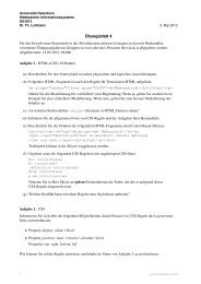
call dim(L) := n the dimension of L. For an example of a two-dimensional lattice with<br />
basis B = {(0,2),(1,1)}, see Figure 2.1.<br />
21
Preliminaries on lattices<br />
000000000000000000000000000000000<br />
111111111111111111111111111111111<br />
00000000000000000000000<br />
11111111111111111111111<br />
0000000000000<br />
1111111111111<br />
000 111<br />
000000000000000000000000000000000<br />
111111111111111111111111111111111<br />
000000000000000000000000000000000<br />
111111111111111111111111111111111<br />
00000000000000000000000<br />
11111111111111111111111<br />
0000000000000<br />
1111111111111<br />
000 111<br />
000000000000000000000000000000000<br />
111111111111111111111111111111111<br />
000000000000000000000000000000000<br />
111111111111111111111111111111111<br />
00000000000000000000000<br />
11111111111111111111111<br />
0000000000000<br />
1111111111111<br />
000 111<br />
000000000000000000000000000000000<br />
111111111111111111111111111111111<br />
000000000000000000000000000000000<br />
111111111111111111111111111111111<br />
00000000000000000000000<br />
11111111111111111111111<br />
0000000000000<br />
1111111111111<br />
000 111<br />
000000000000000000000000000000000<br />
111111111111111111111111111111111<br />
000000000000000000000000000000000<br />
111111111111111111111111111111111<br />
00000000000000000000000<br />
11111111111111111111111<br />
0000000000000<br />
1111111111111 000000000000000000000000000000000<br />
111111111111111111111111111111111<br />
000000000000000000000000000000000<br />
111111111111111111111111111111111<br />
00000000000000000000000<br />
11111111111111111111111<br />
0000000000000<br />
1111111111111 000000000000000000000000000000000<br />
111111111111111111111111111111111<br />
000000000000000000000000000000000<br />
111111111111111111111111111111111<br />
00000000000000000000000<br />
11111111111111111111111<br />
0000000000000<br />
1111111111111 000000000000000000000000000000000<br />
111111111111111111111111111111111<br />
000000000000000000000000000000000<br />
111111111111111111111111111111111<br />
00000000000000000000000<br />
11111111111111111111111<br />
0000000000000<br />
1111111111111 000000000000000000000000000000000<br />
111111111111111111111111111111111<br />
000000000000000000000000000000000<br />
111111111111111111111111111111111<br />
00000000000000000000000<br />
11111111111111111111111<br />
0000000000000<br />
1111111111111 000000000000000000000000000000000<br />
111111111111111111111111111111111<br />
000000000000000000000000000000000<br />
111111111111111111111111111111111<br />
00000000000000000000000<br />
11111111111111111111111<br />
0000000000000<br />
1111111111111 000000000000000000000000000000000<br />
111111111111111111111111111111111<br />
000000000000000000000000000000000<br />
111111111111111111111111111111111<br />
00000000000000000000000<br />
11111111111111111111111<br />
0000000000000<br />
1111111111111 000000000000000000000000000000000<br />
111111111111111111111111111111111<br />
00000000000000000000000<br />
11111111111111111111111<br />
000000000000000000000000000000000<br />
111111111111111111111111111111111<br />
00000000000000000000000<br />
11111111111111111111111<br />
000000000000000000000000000000000<br />
111111111111111111111111111111111<br />
00000000000000000000000<br />
11111111111111111111111<br />
000000000000000000000000000000000<br />
111111111111111111111111111111111<br />
00000000000000000000000<br />
11111111111111111111111<br />
000000000000000000000000000000000<br />
111111111111111111111111111111111<br />
00000000000000000000000<br />
11111111111111111111111<br />
000000000000000000000000000000000<br />
111111111111111111111111111111111<br />
00000000000000000000000<br />
11111111111111111111111<br />
000000000000000000000000000000000<br />
111111111111111111111111111111111<br />
00000000000000000000000<br />
11111111111111111111111<br />
000000000000000000000000000000000<br />
111111111111111111111111111111111<br />
00000000000000000000000<br />
11111111111111111111111<br />
000000000000000000000000000000000<br />
111111111111111111111111111111111<br />
00000000000000000000000<br />
11111111111111111111111<br />
000000000000000000000000000000000<br />
111111111111111111111111111111111<br />
00000000000000000000000<br />
11111111111111111111111<br />
000000000000000000000000000000000<br />
111111111111111111111111111111111<br />
00000000000000000000000<br />
11111111111111111111111<br />
000000000000000000000000000000000<br />
111111111111111111111111111111111<br />
00000000000000000000000<br />
11111111111111111111111<br />
000000000000000000000000000000000<br />
111111111111111111111111111111111<br />
00000000000000000000000<br />
11111111111111111111111<br />
000000000000000000000000000000000<br />
111111111111111111111111111111111<br />
00000000000000000000000<br />
11111111111111111111111<br />
000000000000000000000000000000000<br />
111111111111111111111111111111111<br />
00000000000000000000000<br />
11111111111111111111111<br />
0000000000000<br />
1111111111111<br />
000000000000000000000000000000000<br />
111111111111111111111111111111111<br />
00000000000000000000000<br />
11111111111111111111111<br />
000000000000000000000000000000000<br />
111111111111111111111111111111111<br />
00000000000000000000000<br />
11111111111111111111111<br />
0000000000000<br />
1111111111111<br />
000000000000000000000000000000000<br />
111111111111111111111111111111111<br />
000000000000000000000000000000000<br />
111111111111111111111111111111111<br />
00000000000000000000000<br />
11111111111111111111111<br />
0000000000000<br />
1111111111111<br />
000000000000000000000000000000000<br />
111111111111111111111111111111111<br />
000000000000000000000000000000000<br />
111111111111111111111111111111111<br />
00000000000000000000000<br />
11111111111111111111111<br />
0000000000000<br />
1111111111111<br />
000000000000000000000000000000000<br />
111111111111111111111111111111111<br />
000000000000000000000000000000000<br />
111111111111111111111111111111111<br />
00000000000000000000000<br />
11111111111111111111111<br />
0000000000000<br />
1111111111111<br />
000000000000000000000000000000000<br />
111111111111111111111111111111111<br />
00000<br />
11111 (1,1)<br />
000000000000000000000000000000000<br />
111111111111111111111111111111111<br />
00000000000000000000000<br />
11111111111111111111111<br />
0000000000000<br />
1111111111111<br />
000000000000000000000000000000000<br />
111111111111111111111111111111111<br />
00000<br />
11111 000000000000000000000000000000000<br />
111111111111111111111111111111111<br />
00000000000000000000000<br />
11111111111111111111111<br />
0000000000000<br />
1111111111111<br />
000000000000000000000000000000000<br />
111111111111111111111111111111111<br />
00000<br />
11111 000000000000000000000000000000000<br />
111111111111111111111111111111111<br />
00000000000000000000000<br />
11111111111111111111111<br />
0000000000000<br />
1111111111111<br />
000000000000000000000000000000000<br />
111111111111111111111111111111111<br />
000000000000000000000000000000000<br />
111111111111111111111111111111111<br />
00000000000000000000000<br />
11111111111111111111111<br />
0000000000000<br />
1111111111111 000 111<br />
00000<br />
11111<br />
000000000000000000000000000000000<br />
111111111111111111111111111111111<br />
000000000000000000000000000000000<br />
111111111111111111111111111111111<br />
00000000000000000000000<br />
11111111111111111111111<br />
0000000000000<br />
1111111111111 000 111<br />
00000<br />
11111<br />
000000000000000000000000000000000000000000000<br />
111111111111111111111111111111111111111111111<br />
000000000000000000000000000000000<br />
111111111111111111111111111111111<br />
000000000000000000000000000000000<br />
111111111111111111111111111111111<br />
00000000000000000000000<br />
11111111111111111111111<br />
0000000000000<br />
1111111111111 000 111<br />
00000<br />
11111<br />
000000000000000000000000000000000<br />
111111111111111111111111111111111<br />
000000000000000000000000000000000<br />
111111111111111111111111111111111<br />
00000000000000000000000<br />
11111111111111111111111<br />
0000000000000<br />
1111111111111 000 111<br />
(0,2)<br />
Figure 2.1: <strong>Lattice</strong> with basis B = {(0,2),(1,1)}<br />
By v ∗ 1 ,... ,v∗ n we denote the vectors obtained by applying Gram-Schmidt orthogonalization<br />
to the basis vectors. The determinant of L is defined as<br />
det(L) :=<br />
n�<br />
|v ∗ i |,<br />
where |v | denotes the Euclidean norm of v. Any lattice L has infinitely many bases but<br />
all bases have the same determinant. If a lattice is full rank, det(L) is the absolute value<br />
of the determinant of the (n × n)-matrix whose rows are the basis vectors v1,... ,vn.<br />
Hence if a basis matrix is triangular, the determinant can easily be computed by<br />
multiplying the entries on the diagonal of the basis matrix. In the subsequent sections,<br />
we will mostly deal with triangular basis matrices. In Chapter 7, we will introduce nontriangular<br />
bases but we will reduce the determinant computations for these bases also<br />
to the case of triangular bases.<br />
A well-known result by Minkowski [51] relates the determinant of a lattice L to the<br />
length of a shortest vector in L.<br />
Theorem 3 (Minkowski) Every n-dimensional lattice L contains a non-zero vector v<br />
with |v | ≤ √ n det(L) 1<br />
n.<br />
Unfortunately, the proof of this theorem is non-constructive.<br />
In dimension 2, the Gauss reduction algorithm finds a shortest vector of a lattice<br />
(see for instance [58]). In arbitrary dimension, we can use the famous L 3 -reduction<br />
algorithm of Lenstra, Lenstra and Lovász [44] to approximate a shortest vector. We<br />
prove an upper bound for each vector in an L 3 -reduced lattice basis in the following<br />
theorem. The bounds for the three shortest vectors in an L 3 -reduced basis will be<br />
frequently used in the following chapters.<br />
22<br />
i=1
Preliminaries on lattices<br />
Theorem 4 (Lenstra, Lenstra, Lovász) Let L ∈�n be a lattice spanned by B =<br />
{b1,... ,bn}. The L 3 -algorithm outputs a reduced lattice basis {v1,... ,vn} with<br />
|vi | ≤ 2 n(n−1) 1<br />
4(n−i+1) det(L) n−i+1 for i = 1,... ,n<br />
in time polynomial in n and in the bit-size of the entries of the basis matrix B.<br />
Proof: Lenstra, Lenstra and Lovász [44] showed that the L 3 -algorithm outputs a basis<br />
{v1,... ,vn} satisfying<br />
|vi | ≤ 2 j−1<br />
2 |v ∗ j | for 1 ≤ i ≤ j ≤ n.<br />
For a vector vi, we apply this inequality once for each j, i ≤ j ≤ n, which yields<br />
|vi | n−i+1 ≤<br />
n�<br />
j=i<br />
2 j−1<br />
2 |v ∗ j |. (2.3)<br />
Since L ∈�n , we know that |v ∗ 1 | = |v1 | ≥ 1. For an L 3 -reduced basis, we have<br />
Therefore, we obtain<br />
2|v ∗ j | 2 ≥ |v ∗ j−1 | 2<br />
for 1 < j ≤ n (see [44]).<br />
2 j−1<br />
2 |v ∗ j | ≥ |v∗ 1 | ≥ 1 for 1 ≤ j ≤ n.<br />
We apply the last inequality in order to bound<br />
n�<br />
j=i<br />
2 j−1<br />
2 |v ∗ j | ≤<br />
n�<br />
j=1<br />
2 j−1<br />
2 |v ∗ j | = 2 n(n−1)<br />
4 det(L).<br />
<strong>Using</strong> this inequality together with inequality (2.3) proves the theorem.<br />
23
3 Coppersmith’s method<br />
3.1 Introduction<br />
Every integer that is sufficiently small<br />
in absolute value, must be zero.<br />
In 1996, Coppersmith [18, 19, 20, 21] introduced a method for finding small roots of<br />
modular polynomial equations using the L 3 -algorithm. Since then, the method has<br />
found many different applications in the area of public key cryptography. Interestingly,<br />
besides many results in cryptanalysis [3, 13, 14, 16, 20, 28] it has also been used in the<br />
design of provably secure cryptosystems [62].<br />
We will present Coppersmith’s method in this chapter. Nearly all the results in the<br />
subsequent chapters will be based on Coppersmith’s method. In fact, one can view our<br />
new results as different applications of the method. Since all of our applications belong to<br />
the field of cryptanalytic attacks on the <strong>RSA</strong> cryptosystem, we will first give an informal<br />
example that explains the significance of a modular root finding method in the area of<br />
public key cryptanalysis and here especially for <strong>RSA</strong>.<br />
In public key cryptosystems, we have a public key/secret key pair. For instance in<br />
the <strong>RSA</strong> scheme, the public key is the tuple (N,e) and the secret key is d. The public<br />
key/secret key pair satisfies<br />
ed = 1 + kφ(N), where k ∈Æ.<br />
We see that in the <strong>RSA</strong> scheme, the public key pair (N,e) satisfies a relation with the<br />
unknown parameters d, k and φ(N) = N − (p + q − 1). Hence, we can assign the<br />
unknown values d, k and p+q −1 the variables x, y and z, respectively. Then we obtain<br />
a polynomial<br />
f(x,y,z) = ex − y(N − z) − 1<br />
with the root (x0,y0,z0) = (d,k,p + q − 1) over the integers. Suppose we could find<br />
the root (x0,y0,z0). Then we could solve the following system of two equations in the<br />
unknowns p and q<br />
�<br />
�<br />
�<br />
� p + q − 1 = z0 �<br />
�<br />
� pq = N � .<br />
24
Introduction: Coppersmith’s method<br />
Substituting q = N<br />
p in the first equation gives us the quadratic equation p2 −(z0 +1)p+<br />
N = 0 which has the two solutions p and q.<br />
Hence, finding the root (x0,y0,z0) is polynomial time equivalent to the factorization<br />
of N. Unfortunately, we do not know how to find such a root and since we assume that<br />
factoring is hard, we cannot hope to find an efficient method for extracting (x0,y0,z0) in<br />
general. However, the inability of finding a general solution does not imply that there are<br />
no roots (x0,y0,z0) of a special form for which we can solve the problem in polynomial<br />
time in the bit-length of N. This special form is the point where Coppersmith’s method<br />
comes into the play.<br />
Suppose we had a general method how to find small roots of modular polynomial<br />
equations, where small means that every component of the root is small compared to<br />
the modulus. Could we then discover the unknown solution (x0,y0,z0) of the equation<br />
f(x,y,z) = 0? The obvious problem with this approach is:<br />
The equation f(x,y,z) = 0 is not a modular polynomial equation but an equation<br />
over the integers.<br />
It is easy to come around with this problem: Simply choose one of the known parameters<br />
in f(x,y,z) as the modulus, e.g., we could choose either N or e. Then we obtain<br />
the following modular polynomial equations, respectively:<br />
fN(x,yz) = ex + yz − 1 and fe(y,z) = y(N − z) + 1.<br />
We see that in fN we can treat yz as a new variable. So in fact, both polynomials are<br />
bivariate polynomials. The polynomial fN has the root (d,k(p + q − 1)) modulo N,<br />
whereas the polynomial fe has the root (k,p + q − 1) modulo e. Now the requirement<br />
that the roots of fN and fe should be small compared to the modulus makes sense.<br />
Notice that we have introduced a notation, which we will keep throughout this thesis:<br />
The subscript N of the polynomial fN denotes that fN is evaluated modulo N.<br />
In order to bound the parameter k we observe that<br />
k =<br />
ed − 1<br />
φ(N)<br />
e<br />
< d < d.<br />
φ(N)<br />
Hence, if we choose d to be a small secret value then k is automatically small. Since<br />
the running time of <strong>RSA</strong> decryption with the Repeated Squaring Method of Section 2.1<br />
is O(log d · log 2 N), small values of d speed up the <strong>RSA</strong> decryption/signature process.<br />
Therefore, it is tempting to use small values of d for efficiency reasons.<br />
But small choices of d lead to the two most famous attacks on <strong>RSA</strong> up to now:<br />
Wiener [71] showed in 1990 that values of d < 1<br />
3<br />
N 1<br />
4 yield the factorization of N. In<br />
1− √<br />
1<br />
1999, Boneh and Durfee [12] improved this result to d < N 2 ≈ N0.292 . Interestingly,<br />
both methods can be seen as an application of Coppersmith’s method:<br />
25
Introduction: Coppersmith’s method<br />
• Wiener’s method corresponds to an application of Coppersmith’s method using<br />
the polynomial fN(x,yz). Originally, Wiener presented his results in terms of<br />
continued fractions. We show in Section 4.2 how an application of Coppersmith’s<br />
method using the polynomial fN leads to a two-dimensional lattice L. The shortest<br />
vector in L then yields the factorization of N, whenever the Wiener-bound d <<br />
1<br />
1<br />
3N 4 holds.<br />
• The attack on <strong>RSA</strong> with small secret exponent d due to Boneh-Durfee makes use<br />
of the polynomial fe(y,z) in combination with Coppersmith’s method. This leads<br />
to the improved bound of d < N 0.292 .<br />
In this thesis, we study further applications of Coppersmith’s method. All these applications<br />
have the property that d is not small itself but satisfies a relation with small<br />
unknown parameters:<br />
• A generalization of Wiener’s attack: We present a new method that works if d has<br />
a decomposition d = d1<br />
d2 mod φ(N) into small d1, d2. As an application of this new<br />
approach, we cryptanalyze an <strong>RSA</strong>-type scheme presented in 2001 [73, 74].<br />
• Attacks on unbalanced <strong>RSA</strong> with small CRT-exponent: Here d has a Chinese<br />
Remainder Theorem decomposition d = (dp,dq), where dp = d mod p − 1 is small.<br />
This CRT-property of d is of important practical significance, since one can use<br />
small values of dp, dq in order to speed up the fast Quisquater-Couvreur variant<br />
of <strong>RSA</strong> decryption (see Section 2.1). We show that the factorization of N can be<br />
found whenever the prime factor p is sufficiently large.<br />
• Partial key exposure attacks on <strong>RSA</strong>: We present attacks on <strong>RSA</strong> when parts of<br />
the secret key d are known. For instance suppose that an attacker knows a value<br />
˜d that corresponds to the k least significant bits of d, e.g. d = x · 2 k + ˜ d for some<br />
unknown x. The more bits we know, the smaller is the value of the unknown x.<br />
Thus, one can hope to recover x using Coppersmith’s method whenever sufficiently<br />
many bits of d are known.<br />
For the rest of this chapter, we present Coppersmith’s method. Therefore, we review<br />
in Section 6 Coppersmith’s method in the case of univariate modular polynomial<br />
equations. In the univariate case, Coppersmith’s method provably outputs every root<br />
that is sufficiently small in absolute value. As an important application of the univariate<br />
case, we show a result that was also presented in Coppersmith’s work in 1996 [18]: The<br />
knowledge of half of the most significant bits of p suffice to find the factorization of an<br />
<strong>RSA</strong>-modulus N = pq in polynomial time. Originally, Coppersmith used a bivariate<br />
polynomial equation to show this result. However as we will see, the univariate modular<br />
approach already suffices.<br />
26
The univariate case<br />
In Section 3.4, we present Coppersmith’s extensions to the multivariate polynomial<br />
case. The main drawback of the generalization to the multivariate case is that the<br />
method is no longer rigorous. It depends on some (reasonable) heuristic.<br />
3.2 The univariate case<br />
“Everything should be made as simple as possible,<br />
but not simpler.”<br />
Albert Einstein (1879-1955)<br />
Let us first introduce some helpful notations. Let f(x) := �<br />
i aixi be a univariate<br />
polynomial with coefficients ai ∈�. We will often use the short-hand notation f for<br />
f(x). All terms xi with non-zero coefficients are called monomials. The degree of f<br />
is defined as max{i | ai �= 0}. Let f be a polynomial of degree i, then we call ai the<br />
leading coefficient of f. A polynomial is called monic if its leading coefficient is 1. The<br />
coefficient vector of f is defined by the vector of the coefficients ai. We define the norm<br />
of f as the Euclidean norm of the coefficient vector: |f | 2 := �<br />
multivariate polynomials are analogous.<br />
In this section, we study the following problem:<br />
i a2 i<br />
. The definitions for<br />
Let N be a composite number of unknown factorization and b be a divisor of N,<br />
where b ≥ N β for some known β. Notice that b must not be a prime. Given an<br />
univariate polynomial fb(x) ∈�[X] of degree δ. Find in time polynomial in δ and<br />
in the bit-size of N all roots x0 ∈�of fb(x) modulo b, where |x0| < X for some X.<br />
The goal is to choose the upper bound X for the size of the roots x0 as large as<br />
possible.<br />
First, we consider one important special case of the problem above: The case, where<br />
b = N. We want to point out that this is the case that was studied by Coppersmith in<br />
his original work [20]. However, we think it is convenient to formulate Coppersmith’s<br />
method in a more general framework, since in this more general form we can easily derive<br />
important applications of Coppersmith’s method in the following sections as simple<br />
implications of the results of the problem above. For instance, some results in the<br />
literature — e.g. the factorization algorithm for moduli N = p r q with large r due to<br />
Boneh, Durfee and Howgrave-Graham [16] — use Coppersmith’s method but do not<br />
fit in the original formulation of the problem. To our knowledge, the new formulation<br />
covers all approaches mentioned in the literature.<br />
Nevertheless, let us first give some motivation for the importance of the case b = N.<br />
We do not know how to solve modular polynomial equations, when the factorization of<br />
the modulus N is unknown. Notice that the problem of decrypting an <strong>RSA</strong>-encrypted<br />
message c = m e mod N is the problem of finding the unique positive root x0 = m < N<br />
27
of the polynomial<br />
The univariate case<br />
fN(x) = x e − c mod N.<br />
Under the assumption that inverting the <strong>RSA</strong>-function is hard, we cannot solve this<br />
problem in general. If we knew the factors p and q, we could find the roots of fN(x)<br />
modulo p and modulo q. <strong>Using</strong> the Chinese Remainder Theorem, we could then combine<br />
both solutions and recover x modulo N.<br />
But if we cannot solve the problem for all m ∈�N, then it might be feasible for<br />
especially small values of m. Indeed, it is a well-known protocol failure of <strong>RSA</strong> that one<br />
can recover m in polynomial time whenever m < N 1<br />
e. The reason why this attack works<br />
is simple: Since me < N, we have<br />
m e − c = 0 over�<br />
and not just modulo N. Thus, we can simply take the e th root of c in order to recover<br />
the value of m. Notice that this attack can easily be avoided by padding each message<br />
m with additional bits such that m becomes sufficiently large.<br />
However, the attack above already yields a simple idea how to solve modular univariate<br />
polynomial equations:<br />
Reduce the root finding problem in modular equations to the case of root finding<br />
in equations over the integers.<br />
Thus, the idea is to construct from the polynomial fb(x) with the root x0 ≤ X<br />
modulo b a polynomial f(x) which has the same root x0 over the integers. Then we can<br />
easily find the root x0 by applying standard root finding algorithms to f(x) (take for<br />
instance the Sturm sequence, see [39]).<br />
But how can we transform fb(x) into f(x)? This transformation is exactly the core<br />
of Coppersmith’s method. In the following, we describe Coppersmith’s reduction of the<br />
modular root finding case to root finding case over the integers.<br />
<strong>Reduction</strong> of the modular to the integer case<br />
Recall that we start with the knowledge of the following values:<br />
Known parameters: – the modulus N of unknown factorization with divisor b<br />
Unknown parameters: – the root x0<br />
– the lower bound N β with b ≥ N β<br />
– the polynomial fb(x) with fb(x0) = 0 mod b for some |x0| ≤ X<br />
– the modulus b.<br />
28
The univariate case<br />
In order to construct f(x), we fix an integer m and construct a set G of univariate<br />
polynomials where each polynomial g(x) ∈ G satisfies<br />
g(x0) = 0 mod b m .<br />
Since we do not know the values of x0 and b, we can only use the parameters fb(x) and<br />
N in order to construct the set G. This means that we can choose polynomials of the<br />
form<br />
gi,j(x) = N m−i x j f i b (x) for i = 1,... ,m and some choice of j.<br />
Notice that for each choice of i,j we have gi,j(x0) = 0 mod b m since f i b (x0) = 0 mod b i<br />
and N m−i is a multiple of b m−i .<br />
But then every integer linear combination<br />
f(x) = �<br />
i,j<br />
ai,jgi,j(x) , ai.j ∈�<br />
(3.1)<br />
of polynomials in G also has the root x0 modulo b m . Our goal is to find among these<br />
linear combinations one which has the root x0 not just modulo b m but also over the<br />
integers. But which property does the above linear combination f(x) of polynomials in<br />
G need to satisfy in this case? The most simple idea is to choose the coefficients ai,j<br />
such that f(x) satisfies the relation<br />
|f(x0)| < b m .<br />
Since we know that f(x0) = 0 mod b m and f(x0) ∈�, we can conclude that f(x0) = 0<br />
over the integers. In other words we use the following basic principle that underlies<br />
Coppersmith’s method:<br />
Every integer multiple of b m that is small enough must be zero!<br />
However, there remain two serious problems with the approach so far:<br />
1. How can we find the coefficients ai,j efficiently?<br />
2. How can we check that the relation |f(x0)| < b m is satisfied if we do not know the<br />
values of x0 and b?<br />
Let us first address the second problem. Observe that instead of x0 and b we know bounds<br />
X, Nβ satisfying |x0| ≤ X and b ≥ Nβ . Thus, instead of checking if a polynomial f(x)<br />
is smaller than bm at the point x0, we could check whether the condition |f(X)| < Nβm holds. In other words: We check if f evaluated at a larger point gives some smaller<br />
value. But still this approach makes some problems: Let f(x) := �n−1 i=0 cixi , ci ∈�. We<br />
could be in the case, where we have |f(X)| < Nβm and still |f(x0)| ≥ bm . The reason<br />
29
The univariate case<br />
for that is that the coefficients ci may be negative. Some terms in f(X) may cancel out<br />
where in f(x0) they lead to a large value.<br />
Hence, we cannot evaluate f(x) at the point X directly but we first have to force<br />
all coefficients ci of f(x) to be non-negative by taking the absolute values. <strong>Using</strong> the<br />
triangle inequality, we obtain the following inequalities:<br />
n−1 �<br />
|f(x0)| ≤ |cix i n−1 �<br />
0 | ≤ |ci|X i .<br />
i=0<br />
If we could satisfy the inequality � n−1<br />
i=0 |ci|X i < N βm this would automatically imply<br />
the desired condition |f(x0)| < N βm ≤ b m . We observe that the polynomial<br />
i=0<br />
n−1 �<br />
f(xX) = ci(xX) i<br />
i=0<br />
has the coefficient vector (c0X0 ,c1X 1 ,... ,cn−1X n−1 ). Thus, the term �n−1 i=0 |ci|Xi is<br />
the ℓ1-norm of the coefficient vector of f(xX) and thus by our definition of the norm of<br />
a polynomial |f(xX)|ℓ1 = �n−1 i=0 |ci|Xi . Therefore, our polynomial f(x) has to satisfy<br />
the condition |f(xX)|ℓ1 < bm . Since by switching to the Euclidean norm, we loose at<br />
most a factor of √ n, we could also use the condition √ n · |f(xX)| < bm .<br />
The last condition will be used in the following theorem. We want to point out that<br />
Coppersmith originally did not formulate this condition in terms of polynomial arithmetic.<br />
This convenient and very useful formulation is due to Howgrave-Graham [35] who<br />
revisited Coppersmith’s method. Therefore, the following theorem is due to Howgrave-<br />
Graham although it resembles Coppersmith’s original idea. We think that the different<br />
point of view on Coppersmith’s method due to Howgrave-Graham was one of the reasons<br />
that Coppersmith’s method has found so many applications in cryptography. Therefore<br />
throughout the thesis, we always refer to Howgrave-Graham’s theorem by keeping in<br />
mind that it is a reformulation of Coppersmith’s underlying idea.<br />
Theorem 5 (Howgrave-Graham) Let f(x) be an univariate polynomial with n monomials.<br />
Further, let m be a positive integer. Suppose that<br />
(1) f(x0) = 0 mod b m where |x0| < X<br />
(2) |f(xX)| < bm<br />
√ n<br />
Then f(x0) = 0 holds over the integers.<br />
30
Proof: We have<br />
The univariate case<br />
|f(x0)| = �<br />
cix i 0 ≤ �<br />
|cix i 0|<br />
i<br />
i<br />
≤ �<br />
|ci|X i ≤ √ n|f(xX)| < b m .<br />
But f(x0) is a multiple of b m and therefore it must be zero.<br />
i<br />
Up to this point, we only derived conditions under which a polynomial f(x) has a root<br />
x0, |x0| ≤ X over the integers. Now, we want to show how to construct such a polynomial<br />
f(x). Remember from equation (3.1) that every f(x) which is an integer linear<br />
combination<br />
f(x) = �<br />
ai,jgi,j(x)<br />
i,j<br />
of the polynomials gi,j ∈ G satisfies condition (1) of Howgrave-Graham’s theorem, since<br />
every gi,j satisfies condition (1). Therefore, we have to search among all integer linear<br />
combinations for a polynomial f(x) which also satisfies the second condition of Theo-<br />
rem 5. In other words, we have to search among all integer linear combinations of the<br />
coefficient vectors gi,j(xX) for one vector with Euclidean norm smaller than bm<br />
√ n . But<br />
this means:<br />
Find in the lattice L that is spanned by the coefficient vectors of gi,j(xX) a vector<br />
with Euclidean norm smaller than bm √ .<br />
n<br />
Our goal is to ensure that the L 3 -algorithm finds a vector v with |v | < bm<br />
√ n in L.<br />
Then we could apply the L 3 -algorithm to the basis spanned by the coefficient vectors of<br />
gi,j(xX) and find a sufficiently small vector. Notice that by Theorem 4, the norm of a<br />
shortest vector v in an L 3 -reduced integer basis can by related to the determinant of the<br />
corresponding lattice L with dimension n by<br />
Thus if we could satisfy the inequality<br />
|v | ≤ 2 n−1<br />
4 det(L) 1<br />
n.<br />
2 n−1<br />
4 det(L) 1<br />
n < Nβm<br />
√ n<br />
(3.2)<br />
then we have the desired inequality |v | < Nβm<br />
√ n ≤ bm<br />
√ n , which guarantees that the short-<br />
est vector of an L 3 -reduced basis is sufficiently short to satisfy the second condition in<br />
31
The univariate case<br />
Theorem 5. Notice that inequality (3.2) gives us a very useful condition, since we can<br />
compute from the coefficient vectors of gi,j(xX) the determinant of L.<br />
Furthermore, we observe that det(L) depends on the values of N and X, since the<br />
gi,j depend on these parameters. Thus, inequality (3.2) gives us a restriction on the size<br />
of X which can be used in Coppersmith’s method. Remember that X is an upper bound<br />
for the size of the roots x0 that can be found.<br />
In our application of Coppersmith’s method, we will often be in the case where N<br />
is very large (e.g. in the order of 2 1000 ), whereas the lattice dimension n is negligible<br />
compared to N (in the order of 100). Therefore, we can often neglect the terms that<br />
depend only on n, which simplifies condition (3.2) to the elegant form<br />
det(L) < N βmn . (3.3)<br />
Since we want to maximize the size of X, we have to choose the gi,j such that det(L)<br />
is as small as possible. We can give an even more quantitative statement which gi,j are<br />
helpful in order to optimize the size of X:<br />
Suppose we have a basis that satisfies inequality (3.3). Assume we assign a new<br />
coefficient vector of some gi,j(xX) to the basis. This increases the lattice dimension n<br />
by 1, which in turn increases the right-hand side of inequality (3.3) by a factor of N βm .<br />
Hence, if the contribution of the new vector to the determinant is at most a factor of<br />
N βm , then inequality (3.3) still holds. Moreover, if the contribution to det(L) is significantly<br />
less than N βm , then we can slightly increase det(L) and the condition (3.3) will<br />
still be valid. But the ability to increase the determinant means that we can increase<br />
the value of X. Hence:<br />
Every basis vector that contributes to det(L) with a factor smaller than N βm is<br />
helpful !<br />
This criterion will be used throughout the thesis in order to optimize the choices<br />
of basis vectors. Normally, we will use lattice bases whose bases matrices are in lower<br />
triangular form. In this case, the criterion means that every basis vector with diagonal<br />
entry smaller than N βm is helpful, but the criterion also holds for non-triangular bases.<br />
Let us briefly summarize Coppersmith’s method for the univariate case in some<br />
informal way. We will later specify the values of the parameters that are used here.<br />
32
✬<br />
✫<br />
The univariate case<br />
Coppersmith Method in the univariate case (informally)<br />
INPUT: – Polynomial fb(x) of degree δ<br />
– Modulus N of unknown factorization which is a multiple of b and a<br />
lower bound b ≥ N β<br />
Step 1: Fix an integer m (depending on N, β and δ) and construct a set G of<br />
univariate polynomials, where each gi(x) ∈ G satisfies<br />
g(x) = 0 mod b m .<br />
Step 2: Construct the lattice L from the polynomials gi(x) ∈ G: The basis vectors<br />
of L are the coefficient vectors of gi(xX), where X is chosen such that the<br />
L3 b -algorithm finds a vector with norm smaller than m<br />
dim(L) in L. The size of<br />
X is a function of the parameters N, β and δ.<br />
Step 3: Apply the L 3 -algorithm to the lattice bases. Let v be the shortest vector in<br />
the L 3 -reduced bases. The vector v is the coefficient vector of some polynomial<br />
f(xX). Construct f(x) from v.<br />
OUTPUT: Polynomial f(x) with f(x0) = 0 over�whenever fb(x0) = 0 mod b<br />
and |x0| ≤ X<br />
Notice that every step can be done in time polynomial in the input size.<br />
We can find all roots of f(x) in�by a standard root finding algorithm. We want<br />
to point out that f(x) may have more roots in�than fb(x) modulo b. However, the<br />
number of roots is bounded by the degree of f(x) and the desired roots of fb(x) with<br />
|x0| ≤ X must be among the roots of f(x).<br />
Coppersmith’s Theorem<br />
Now, we will apply Coppersmith’s method on arbitrary univariate, monic polynomials<br />
fb(x) of degree δ. Normally, the property that fb(x) is monic is no restriction in practice.<br />
Assume that fb(x) has a leading coefficient aδ �= 1, then one could compute the inverse<br />
a −1<br />
δ of aδ modulo N. Since N is a multiple of b, the value a −1<br />
δ will also be an inverse of<br />
ai modulo b and we can make fb(x) monic by multiplying with this inverse. The only<br />
problem that might occur is the case when aδ and the modulus N share a non-trivial<br />
greatest common divisor, since then a −1<br />
δ does not exist. However, if we assume that N<br />
is hard to factor (which will always be the case in our applications), then either this case<br />
does not occur or we have found a non-trivial factor of N.<br />
The following theorem of Coppersmith states that for a monic polynomial fb(x) of<br />
33<br />
✩<br />
✪
The univariate case<br />
degree δ, all roots x0 with |x0| ≤ N β2<br />
δ can be found in polynomial time.<br />
Theorem 6 (Coppersmith) Let N be an integer of unknown factorization, which has<br />
a divisor b ≥ N β . Furthermore, let fb(x) be an univariate, monic polynomial of degree<br />
δ. Then we can find all solutions x0 for the equation fb(x) = 0 mod b with<br />
in time polynomial in (log N,δ, 1<br />
ǫ ).<br />
|x0| ≤ 1 β2<br />
N δ<br />
2 −ǫ<br />
Proof: Define X := 1<br />
2<br />
method. In the first step, we fix an integer m such that<br />
N β2<br />
δ −ǫ . Now, we successively apply the steps of Coppersmith’s<br />
� �<br />
β2 7β<br />
m ≥ max , . (3.4)<br />
δǫ δ<br />
Notice that for ǫ ≤ 1<br />
7β this implies that we can use the value<br />
� �<br />
β2 m = .<br />
δǫ<br />
Next, we choose a set G of polynomials, where each polynomial has a root x0 modulo b m<br />
whenever fb(x) has the root x0 modulo b. In our case, we include in G the polynomials<br />
N m , xN m , x 2 N m , ... x δ−1 N m ,<br />
N m−1 f, xN m−1 f, x 2 N m−1 f, ... x δ−1 N m−1 f,<br />
N m−2 f 2 , xN m−2 f 2 , x 2 N m−2 f 2 , ... x δ−1 N m−2 f 2 ,<br />
.<br />
.<br />
.<br />
Nf m−1 , xNf m−1 , x 2 Nf m−1 , ... x δ−1 Nf m−1 .<br />
Additionally, we take the polynomials<br />
f m ,xf m ,x 2 f m ,... ,x t−1 f m<br />
for some t that has to be optimized as a function of m.<br />
Note that by our ordering the k th polynomial of G is a polynomial of degree k. Thus,<br />
it introduces the new monomial x k . We could also write the choice of our polynomials<br />
in G in a more compact form. Namely, we have chosen the polynomials<br />
gi,j(x) = x j N i f m−i (x) for i = 0,... ,m − 1, j = 0,... ,δ − 1 and<br />
hi(x) = x i f m (x) for i = 0,... ,t − 1.<br />
34<br />
.
The univariate case<br />
In Step 2 of Coppersmith’s method, we construct the lattice L that is spanned by the<br />
coefficient vectors of gi,j(xX) and hi(xX). As we noticed before, we can order the<br />
polynomials gi,j and hi in strictly increasing order of their degrees k, i.e., each polynomial<br />
introduces exactly one new monomial xk . Therefore, the basis B of L, that has as row<br />
vectors the coefficient vectors of gi,j(xX) and hi(xX), has the property that it can be<br />
written as a lower triangular matrix. Let n := δm + t, then we write B as the following<br />
(n × n)-matrix1 :<br />
⎛<br />
⎜<br />
⎝<br />
N m<br />
N m X<br />
. ..<br />
. ..<br />
. ..<br />
N m X δ−1<br />
. ..<br />
− − . . . − . . . NX δm−δ<br />
− . . . − . . . − NX δm−δ+1<br />
. ..<br />
. ..<br />
. ..<br />
. ..<br />
. ..<br />
− . . . − − . . . NX δm−1<br />
− − . . . − . . . − − − − X δm<br />
− . . . − . . . − − − − − X δm+1<br />
. ..<br />
. ..<br />
. ..<br />
. ..<br />
. ..<br />
. ..<br />
. ..<br />
− − − − − − . . . X δm+t−1<br />
Note that we can easily compute the determinant of L since B is in lower triangular<br />
form. Therefore, det(L) is simply the product of all entries on the diagonal:<br />
det(L) = N 1<br />
2 δm(m+1) X 1<br />
2 n(n−1) . (3.5)<br />
Now we want to optimize the parameter t, which is equivalent to the optimization of<br />
n = δm+t. Remember that in the discussion for Coppersmith’s method, we argued that<br />
every vector which contributes to the determinant by a factor less than b m is helpful. In<br />
our setting this means that we have to ensure that the entries of the coefficient vectors<br />
hi(xX) on the diagonal are all less than b m , i.e., we have the condition<br />
X n−1 < b m .<br />
Since Xn−1 β2<br />
( < N δ −ǫ)(n−1) < N β2<br />
δ n and b ≥ Nβ this condition is satisfied for the choice<br />
n ≤ δ<br />
β m.<br />
According to (3.4), we can choose m as the maximum of<br />
� β 2<br />
δǫ<br />
. ..<br />
�<br />
7β<br />
, δ<br />
roundings). Then, we immediately have a bound for the lattice dimension<br />
�<br />
β<br />
n = max<br />
ǫ ,7<br />
�<br />
,<br />
. ..<br />
. ..<br />
(here we neglect<br />
1 Here we use the following notation: Every non-specified entry is zero. The entries marked with “-”<br />
may be non-zero, but the determinant of the lattice does not depend on their values<br />
35<br />
⎞<br />
⎟<br />
⎠
The univariate case<br />
which is polynomial in 1<br />
ǫ . Since the bit-size of the entries in B can be bounded by<br />
(δ + m)log N ≤ (δ + n)log N, the L3-algorithm operated on B in time polynomial in<br />
log N, δ and 1<br />
ǫ . Now, we want to prove that the L3-algorithm also finds a vector which<br />
is sufficiently short.<br />
In order to apply the theorem of Howgrave-Graham (Theorem 5), we have to ensure<br />
that the L3-algorithm finds a vector in L with norm smaller than bm √ . Since the L<br />
n 3- algorithm finds a vector v in an n-dimensional lattice with |v | ≤ 2 n−1<br />
4 det(L) 1<br />
n, we have<br />
to satisfy the condition<br />
2 n−1<br />
4 det(L) 1<br />
n < bm<br />
√ n .<br />
<strong>Using</strong> the term for det(L) in (3.5) and the fact b ≥ N β , we obtain the new condition<br />
This gives us a condition on the size of X:<br />
N δm(m+1)<br />
2n X n−1 n−1<br />
− 2 ≤ 2 4 n −1 2N βm .<br />
X ≤ 2 −1<br />
1<br />
2n<br />
−<br />
n−1N 2βm<br />
n−1<br />
− δm(m+1)<br />
n(n−1) .<br />
1<br />
n<br />
− −log<br />
Notice that n n−1 = 2 n−1 ≥ 2−1 2 for n ≥ 7. Therefore, our condition simplifies to<br />
X ≤ 1<br />
2<br />
Remember that we made the choice X = 1<br />
2<br />
the theorem, it suffices to show that<br />
2βm δm(m+1)<br />
−<br />
N n−1 n(n−1) .<br />
2βm<br />
n − 1 − δm2 (1 + 1<br />
m )<br />
n(n − 1)<br />
N β2<br />
δ −ǫ . Hence in order to finish the proof of<br />
≥ β2<br />
δ<br />
− ǫ.<br />
We obtain a lower bound for the left-hand side by multiplying with n−1<br />
n<br />
substitute n = δ<br />
βm which gives us<br />
This simplifies to<br />
2 β2<br />
δ<br />
− β2<br />
δ<br />
− β2<br />
δ<br />
�<br />
1 + 1<br />
�<br />
≥<br />
m<br />
β2<br />
− ǫ.<br />
δ<br />
1<br />
· ≥ −ǫ.<br />
m<br />
. Then, we<br />
This in turn gives as the condition m ≥ β2<br />
δǫ , which holds by the choice of m that we<br />
made in (3.4).<br />
Let us briefly summarize the whole algorithm which finds all roots of fb(x) modulo<br />
b that are in absolute value smaller than X.<br />
36
✬<br />
The univariate case<br />
Coppersmith’s method in the univariate case<br />
INPUT: – Polynomial fb(x) of degree δ.<br />
– Modulus N of unknown factorization which is a multiple of b and a<br />
lower bound b ≥ N β<br />
Step 1: Choose the smallest integer m such that m ≥ max<br />
Compute t = ⌊δm( 1<br />
β − 1)⌋.<br />
Compute the polynomials<br />
OUTPUT: Set R, where x0 ∈ R whenever fb(x0) = 0 mod b for an |x0| ≤ X.<br />
✫<br />
� β 2<br />
δǫ<br />
�<br />
7β<br />
, δ .<br />
gi,j(x) = x j N i f m−i (x) for i = 0,... ,m − 1, j = 0,... ,δ − 1 and<br />
hi(x) = x i f m (x) for i = 0... t − 1.<br />
Step 2: Compute the bound X = ⌈N β2<br />
δ −ǫ ⌉. Construct the lattice basis B, where<br />
the basis vectors of B are the coefficient vectors of gi,j(xX) and hi(xX).<br />
Step 3: Apply the L 3 -algorithm to the lattice bases B. Let v be the shortest vector<br />
in the L 3 -reduced bases. The vector v is the coefficient vector of some<br />
polynomial f(xX). Construct f(x) from v.<br />
Step 4: Find the set R of all roots of f(x) over the integers. For every root x0 ∈ R<br />
check whether gcd(N,fb(x0)) ≥ N β . If this condition is not satisfied then<br />
remove x0 from R.<br />
As we noticed before, all steps of the algorithm can be done in time polynomial in<br />
, which concludes the proof of the theorem.<br />
log N, δ and 1<br />
ǫ<br />
One should notice that the polynomial f(x) that we construct in Coppersmith’s<br />
method may contain integer roots that are not roots of fb(x) modulo b. It is easy to<br />
see that one could add an additional integer root a ∈�to f(x) by multiplying with the<br />
linear term (x − a). Therefore, we use in Step 4 of the algorithm in Theorem 6 a simple<br />
test whether fb(x0) is really a divisor of N of size at least Nβ . In the case where b is<br />
prime and β ≥ 1<br />
2 , b is the unique divisor of N with b ≥ Nβ . Therefore in this case, the<br />
set R of integer roots of f(x) contains exactly the roots of fb(x) modulo b. If β < 1<br />
2 , R<br />
may contain roots of fb(x) modulo some other divisor q > Nβ of N. Since we do not<br />
know b, we might have problems to identify the roots of fb(x) modulo b. However, for<br />
all of our applications it will suffice to know only one small root of fb(x) modulo b and<br />
37<br />
✩<br />
✪
this property will be easily testable.<br />
The univariate case<br />
It is also worth noticing the following point: The approximation factor of 2 n−1<br />
4 for the<br />
shortest vector coming from the L 3 -algorithm is exponentially in the lattice dimension<br />
n, but this factor essentially translates in the analysis of Theorem 6 to the term 1<br />
2 for<br />
the upper bound of the size of the roots x0. Thus, computing a shortest vector instead<br />
of an L 3 -approximate version would only improve the bound by a factor of roughly 2<br />
(i.e., only one bit).<br />
Moreover, the following theorem is a direct implication of Theorem 6 and shows<br />
how we can easily remove the terms 1<br />
2 and ǫ from the upper bound on x0 by a simple<br />
brute-force search.<br />
Theorem 7 (Coppersmith) Let N be an integer of unknown factorization, which has<br />
a divisor b ≥ N β . Let fb(x) be an univariate, monic polynomial of degree δ. Furthermore,<br />
let cN be a function that is upper-bounded by a polynomial in log N. Then we can find<br />
all solutions x0 for the equation fb(x) = 0 mod b with<br />
in time polynomial in (log N,δ).<br />
|x0| ≤ cNN β2<br />
δ<br />
Proof: An application of Theorem 6 with the parameter choice ǫ = 1<br />
we can find all roots x0 with<br />
in time polynomial in log N and δ.<br />
|x0| ≤ 1 β2<br />
N δ<br />
4<br />
log N<br />
shows that<br />
In order to find all roots that are of size at most cNN β2<br />
δ in absolute value, we divide<br />
the interval [−cNN β2<br />
δ ,cNN β2<br />
δ ] into 4cN subintervals of size 1<br />
2<br />
N β2<br />
δ centered at some xi.<br />
For each subinterval with center xi, we apply the algorithm of Theorem 6 to the polynomial<br />
fb(x − xi) and output the roots in this subinterval.<br />
For completeness reasons and since it is one of the most interesting cases of Coppersmith’s<br />
method, we explicitly state the special case b = N and cN = 1, which is given in<br />
the work of Coppersmith [20].<br />
Theorem 8 (Coppersmith) Let N be an integer of unknown factorization. Furthermore,<br />
let fN(x) be an univariate, monic polynomial of degree δ. Then we can find all<br />
solutions x0 for the equation fN(x) = 0 mod N with<br />
in time polynomial in (log N,δ).<br />
|x0| ≤ N 1<br />
δ<br />
38
Applications of Coppersmith’s method in the univariate case<br />
In the following section, we state some of the most important applications of Coppersmith’s<br />
method when applied to the <strong>RSA</strong> cryptosystem.<br />
3.3 Applications of Coppersmith’s method in the univariate<br />
case<br />
“How thoroughly it is ingrained in mathematical science that<br />
every real advance goes hand in hand with the invention of<br />
sharper tools and simpler methods which, at the same time,<br />
assist in understanding earlier theories and in casting aside<br />
some more complicated developments”.<br />
David Hilbert (1862-1943)<br />
Attacking <strong>RSA</strong> with small e by knowing parts of the message:<br />
In the introduction to this section, we showed an easy protocol failure of the <strong>RSA</strong><br />
cryptosystem with small encryption exponent e. Assume that we encode a message<br />
m < N 1<br />
e. Since for the ciphertext c = me < N the modulo N reduction does not affect<br />
the computation of c, we can easily recover m by computing the eth root of c over the<br />
integers.<br />
Now consider the following problem:<br />
Suppose that m = M + x for some known part M of the message and some<br />
unknown part x ≤ N 1<br />
e. Can we still recover m?<br />
This situation occurs in the case of so-called stereotyped messages: Assume we already<br />
know a part M of the message which is always the same, for example M corresponds<br />
to ”Good morning to everybody. Todays session-key is:”. The unknown part x<br />
may consist of the words “very secret”. One should notice that <strong>RSA</strong> is frequently used<br />
for encrypting session-keys which in turn are then used in symmetric crypto-schemes.<br />
But symmetric crypto-schemes often need keys of length at most 80 bits. Hence, the<br />
above situation, where the unknown part x is smaller than the e th root of the modulus<br />
N can easily occur in practice when <strong>RSA</strong> is used with small exponent e (for instance<br />
with the frequently used choice e = 3).<br />
Now, let us apply Coppersmith’s method to this problem. An application of Theorem<br />
8 immediately yields the following result.<br />
Theorem 9 (Coppersmith) Let (N,e) be an <strong>RSA</strong> public key. Furthermore, let c :=<br />
(M + x0) e mod N be an <strong>RSA</strong>-encrypted message with known M and unknown x0, where<br />
|x0| ≤ N 1<br />
e.<br />
Then we can find x0 in time polynomial in log N and e.<br />
39
Proof: Define<br />
Applications of Coppersmith’s method in the univariate case<br />
fN(x) := (M + x) e − c,<br />
which is an univariate monic polynomial of degree e with the small root x0, |x0| ≤ N 1<br />
e<br />
modulo N. An application of Theorem 8 proves the claim.<br />
One should notice that an analogous result holds in the case where the unknown part<br />
x is somewhere in the middle of the message, i.e., m = M + x2 k + M ′ when x begins at<br />
the k + 1 st least significant bit. Observe that we need a small modification in the proof<br />
of Theorem 9, since fN(x) = (M + x2 k + M ′ ) e − c is not a monic polynomial. However<br />
the polynomial 2 −ke fN(x) mod N is monic. Note that the inverse of 2 ke modulo N must<br />
exist since <strong>RSA</strong>-moduli are odd. Therefore, we can apply Theorem 8 to the new monic<br />
polynomial.<br />
Factoring <strong>RSA</strong>-moduli N = pq by knowing half of the bits of p<br />
In other scenarios, an attacker might not get parts of the message, but parts of one of<br />
the factors p, q of the modulus N = pq. For example in the Vanstone-Zuccherato IDbased<br />
<strong>RSA</strong> encryption scheme [69], a person’s identity is encoded in his <strong>RSA</strong> modulus.<br />
Vanstone and Zuccherato proposed one variant, where an 1024-bit N is created such<br />
that 264 of the most significant bits of p are publically specified.<br />
We will now present an attack — also due to Coppersmith — that finds the factorization<br />
of N = pq, provided that one knows half of the bits of p. Here we assume wlog<br />
that p > q. This result breaks the above variant of the Vanstone-Zuccherato scheme.<br />
Here again, we will present the results of Coppersmith in a slightly more general<br />
form than originally stated in Coppersmith’s work [20], since we will make use of this<br />
more general form in the subsequent chapters of the thesis. We obtain Coppersmith’s<br />
original result in the following theorem for the special case k = 1.<br />
Theorem 10 (Coppersmith: MSBs of kp) Let N = pq with p > q. Furthermore, let<br />
k be an (unknown) integer that is not a multiple of q. Suppose we know an approximation<br />
˜p of kp with<br />
|kp − ˜p | ≤ 2N 1<br />
4.<br />
Then we can find the factorization of N in time polynomial in log N.<br />
Proof: Define the univariate polynomial<br />
fp(x) := x + ˜p,<br />
which has the root x0 = kp − ˜p modulo p with |x0| ≤ 2N 1<br />
4. The polynomial fp(x) has<br />
degree δ = 1 and we know a lower bound of p ≥ N 1<br />
2 since p > q. Therefore, we can<br />
apply Theorem 7 with the parameter choice β, δ and cN = 2, which gives us the root x0.<br />
40
Applications of Coppersmith’s method in the univariate case<br />
But then we can compute f(x0) = kp. Since k is not a multiple of q, the computation<br />
of gcd(N,f(x0)) yields p. This concludes the proof of the theorem.<br />
We obtain Coppersmith’s original result for the special case k = 1 (here we also remove<br />
the factor 2).<br />
Theorem 11 (Coppersmith: MSBs of p) Let N = pq with p > q. Suppose we know<br />
an approximation ˜p of p with<br />
|p − ˜p | ≤ N 1<br />
4<br />
Then we can find the factorization of N in time polynomial in log N.<br />
Let us give an interpretation of the result in Theorem 11: We can assume for simplicity<br />
that ˜p represents half of the most significant bits of p. Then Coppersmith’s method<br />
finds the rest of the bits of p in polynomial time and hence the factorization of N.<br />
But what happens if an attacker gets half of the least significant bits of p? Analogous<br />
to the case of MSBs of p, one can show similar results when an amount of half of the<br />
bits for any intermediate consecutive bits are unknown. We will only state the result<br />
for the least significant bits of p. A generalization to intermediate consecutive bits is<br />
straight-forward, but we consider the case of intermediate bits neither here nor in the<br />
subsequent sections of this thesis.<br />
In the following theorem, we assume that we know p modulo some sufficiently large<br />
M. In order to interpret this assumption, we can look at the special case M = 2 i : This<br />
means that we know the i least significant bits of p. However, the formulation of the<br />
theorem is more general by allowing arbitrary values of M as long as they are sufficiently<br />
large.<br />
Theorem 12 (Coppersmith: LSBs of p) Let N = pq where p, q are of the same<br />
bit-size with p > q. Suppose we know p0 and M satisfying<br />
p0 = p mod M and M ≥ N 1<br />
4.<br />
Then we can find the factorization of N in time polynomial in log N.<br />
Proof: Define the univariate polynomial<br />
fp(x) := xM + p0.<br />
Since p0 = p mod M, the term x0 = p−p0<br />
M is an integer. Observe that fp(x0) = p and<br />
hence x0 is a root of fp(x) modulo p. But in order to apply Theorem 7, we need to have<br />
a monic polynomial. Therefore, we compute the inverse M −1 of M modulo N. If this<br />
inverse does not exist then gcd(N,M) yields the factorization of N.<br />
41
Applications of Coppersmith’s method in the univariate case<br />
Next, we compute the monic polynomial<br />
f ′ p (x) = M −1 fp(x) mod N<br />
with the same root x0 = p−p0<br />
M modulo p. Now, we have to bound the size of |x0|. We<br />
know that q < √ N < p < 2 √ N, since p and q are of the same bit-size. <strong>Using</strong> M ≥ N 1<br />
4<br />
yields<br />
|x0| =<br />
p − p0<br />
M<br />
1<br />
≤ 2N 4.<br />
Since f ′ 1<br />
p (x) has degree 1 and p ≥ N 2, we can apply Theorem 7 with the parameter<br />
choice δ = 1, β = 1<br />
2 and cN = 2. We obtain x = p−p0<br />
M from which we can easily derive<br />
p. This concludes the proof of the theorem.<br />
Extensions to moduli of the form N = pÖq<br />
Recently, there were a number of cryptosystems proposed that rely on the difficulty<br />
to factor an modulus of the form N = p r q. For instance, Fujioke, Okamoto and<br />
Miyaguchi [30] use a modulus N = p 2 q in an electronic cash scheme. Okamoto and<br />
Uchiyama [54] presented a public-key cryptosystem that is provably as secure as factoring<br />
a modulus of the form N = p 2 q.<br />
In 1998, Takagi [67] observed that the <strong>RSA</strong> decryption process can be performed<br />
significantly faster using moduli of the form N = p r q for some integer r. Takagi’s scheme<br />
can be viewed as an extension of the Quisquater-Couvreur method (see Section 2.1):<br />
Similarly, one uses the decryption exponents dp = d mod p − 1 and dq = d mod q − 1 to<br />
compute m d mod p and m d mod q. The only difference is that one calculates the term<br />
m d mod p r from m d mod p using Hensel lifting before the Chinese Remainder Theorem is<br />
applied. The running time of Hensel lifting is negligible compared to the exponentiations.<br />
Since p and q can be chosen of smaller bit-size than in the original <strong>RSA</strong>-scheme, one<br />
gains performance.<br />
In 1999, Boneh, Durfee and Howgrave-Graham [16] showed that moduli of the form<br />
N = p r q should be handled with care. Their result generalizes Coppersmith’s Theorem<br />
(Theorem 10) to moduli of the form N = p r q. In fact, the following theorem is stated<br />
in the original work of Boneh, Durfee and Howgrave-Graham for the special case k = 1,<br />
but we formulate it in a slightly more general way, since we will use this generalization<br />
later.<br />
Theorem 13 (BDH) Let N = p r q, where r is a known constant and p, q are of the<br />
same bit-size. Let k be an (unknown) integer that is not a multiple of p r−1 q. Suppose<br />
we know an integer ˜p with<br />
Then N can be factored in polynomial time.<br />
|kp − ˜p | ≤ N r<br />
(r+1) 2 .<br />
42
Applications of Coppersmith’s method in the univariate case<br />
Proof: Define the univariate monic polynomial<br />
fp r(x) := (x + ˜p)r .<br />
Then f(x0) = (kp) r = 0 mod pr for the root x0 = kp − ˜p with |x0| ≤ N r<br />
(r+1) 2 .<br />
In order to use Coppersmith’s Theorem for monic univariate polynomials (Theorem<br />
7), we have to specify the degree δ = r of fpr(x) and a lower bound Nβ for the<br />
divisor pr of N. Since p > 1<br />
2q, we know that pr+1 = Np 1<br />
q > 2N. This implies<br />
p r �<br />
1<br />
><br />
2 N<br />
� r<br />
r+1<br />
> 1 r<br />
N r+1<br />
2<br />
Hence we can define β := r<br />
r+1 log N . An application of Theorem 7 with the parameter<br />
choice δ, β and cN = 2 shows that we can find all roots that are of absolute value at<br />
most<br />
− 1<br />
2N β2<br />
δ = 2N r 2 1<br />
(r+1) 2 − + (r+1)log N r log2 N ≥ 2N r 1<br />
r<br />
(r+1) 2 −log N = N (r+1) 2<br />
Thus, we can find the value x0 = kp − ˜p which then in turn gives us the value of kp.<br />
Since k is not a multiple of pr−1q, we know that kp is not a multiple of N. Therefore<br />
gcd(N,kp) is either of the form pi or of the form qpj for some integers i ≤ r, j < r. If<br />
we obtain pi then we can find p by guessing i and computing the ith root of pi . In the<br />
case qpj , we compute N<br />
qpj and further proceed as in the first case. Hence, we obtain the<br />
complete factorization of N which concludes the proof of the theorem.<br />
Let us briefly discuss the implications of Theorem 13 in terms of the fraction of bits of<br />
p that is sufficient to factor N, i.e., we only consider the special case where k = 1. Since<br />
N is of size roughly p r+1 , one could also formulate the theorem for an approximation ˜p<br />
with<br />
|p − ˜p | ≤ p r<br />
r+1.<br />
Thus, we need an amount of roughly 1<br />
r+1 of the bits of p in order to factor N. That<br />
means for the case r = 1, we need half of the most significant bits of p, which is exactly<br />
Coppersmith’s result. So for example if N is an 1000-bit modulus then we need about<br />
250 bits of p. But for r = 2, we need only one third of the bits of p. Again, if N is 1000<br />
bit then p, q are of size 333 bit and we only need to know 111 bit.<br />
Boneh, Durfee and Howgrave-Graham remarked that for<br />
� �<br />
log N<br />
r = Ω ,<br />
log log N<br />
log log N<br />
a fraction of O( log N ) of the bits of p is sufficient. But this is a total amount of<br />
O(log log N) bits, which in turn can be guessed in time O(log N). Therefore, moduli<br />
of the form N = prq can be factored in time polynomial in the bit-length of N if<br />
log N<br />
r = Ω( ). However in cryptographic applications, r is normally a small constant.<br />
log log N<br />
43
3.4 The multivariate case<br />
The multivariate case<br />
“When the mathematician says that such and such a proposition<br />
is true of one thing, it may be interesting, and it is<br />
surely safe. But when he tries to extend his proposition to<br />
everything, though it is much more interesting, it is also<br />
much more dangerous.”<br />
E. Kasner and J. <strong>New</strong>man<br />
A very natural question is whether one can extend Coppersmith’s to the case of multivariate<br />
modular polynomial equations. Hence, we will study here the following problem:<br />
Let N be a composite number of unknown factorization and b be a divisor of N,<br />
where b ≥ N β for some known β. Given a polynomial fb(x1,... ,xk) ∈�[x1,...,xk]<br />
with degree δi in each variable xi. Find in time polynomial in (log N,maxi{δi},k)<br />
all roots (r1,... ,rk) ∈�k of fb(x1,...,xk) modulo b, where |ri| < Xi for some<br />
bounds Xi, i = 1,... ,k.<br />
In principle there is no problem in applying Coppersmith’s methodology from the<br />
previous section that transforms modular polynomials into integer polynomials with the<br />
same small root. That is, we can construct from fb(x1,...,xr) a polynomial f(x1,... ,xr)<br />
with the same small root over the integers and not just modulo b.<br />
We can explicitly state a condition on the upper bounds X1,... ,Xk which tells us<br />
when this reduction from the modular to the integer case succeeds. This condition is<br />
given in the following Lemma due to Howgrave-Graham which is a direct generalization<br />
of Theorem 5 to the multivariate case.<br />
Theorem 14 (Howgrave-Graham) Let f(x1,...,xk) be a polynomial in k variables<br />
with n monomials. Further, let m be a positive integer. Suppose that<br />
(1) f(r1,... ,rk) = 0 mod b m where |ri| < Xi, i = 1,... ,k<br />
(2) |f(x1X1,...,xkXk)| < bm<br />
√ n<br />
Then f(r1,... ,rk) = 0 holds over the integers.<br />
The proof of Theorem 14 is completely analogous to the proof of Theorem 5 in the<br />
previous section. Therefore, we omit it. We will use Theorem 14 frequently in the<br />
subsequent chapters of this thesis in the bivariate and trivariate case.<br />
Up to now, everything works completely similar to the univariate modular case. But<br />
assume that we manage to construct a polynomial f(x1,...,xk) with a small root over<br />
the integers, then there remains a serious problem:<br />
Problem: How can we extract the integer roots of f(x1, x2, . . . , x�)?<br />
44
The multivariate case<br />
Whereas root finding for univariate polynomials can be done in time polynomial in<br />
the input-size, one cannot solve the problem for multivariate polynomials in general.<br />
A simple reason for the impossibility of an efficient solution is the number of possible<br />
solutions. By a fundamental theorem of algebra, the number of integer solutions of an<br />
univariate polynomial f(x) is bounded by its degree. Now consider for instance the<br />
bivariate polynomial<br />
f1(x,y) := x − y.<br />
This polynomial has infinitely many integer solutions which all lie on the line y = x.<br />
Therefore, one cannot enumerate the solutions.<br />
Let us consider a second bivariate polynomial f2(x,y) := x+y −2. The integer roots<br />
of this polynomial lie on the line y = 2 − x, which crosses the line y = x in the point<br />
(x0,y0) = (1,1). Thus, the point (x0,y0) is a common zero of both polynomials. Can<br />
we find common zeros of bivariate polynomials in general? Then one could generalize<br />
Coppersmith’s method in the following way:<br />
Instead of finding just one polynomial f(x1,...,xk) that has some small root<br />
(r1,...,rk) over the integers, we use the L 3 -algorithm in order two find k different<br />
polynomials with the same small root over the integers. Then we compute the<br />
common roots of all polynomials.<br />
Unfortunately, this approach cannot work in general. Let us consider the polynomial<br />
f3(x,y) := x 2 − y 2 . Since gcd(f1,f3) = f1, the common zeros of f1 and f3 are the roots<br />
of the polynomial f1. Hence it seems that we did not gain very much. However, it might<br />
be possible to extract common roots if the number of common roots is not too large.<br />
The resultant heuristic<br />
Let us look at projections of the common roots on one variable. Define<br />
Px := {x ∈�| There is an y ∈�such that f1(x,y) = f2(x,y) = 0}.<br />
Then Px is the projection of the common roots of f1 and f2 onto the x-coordinate. It<br />
remains to show that we can efficiently compute the set Px. This can be done using<br />
resultants of polynomials (for an introduction into the theory of resultants see [22, 23,<br />
72]).<br />
Let r(x) := resy(f1,f2) be the resultant of f1 and f2 with respect to the variable<br />
y. Then r(x) is an univariate polynomial in the variable x, which can be efficiently<br />
computed as the determinant of a Sylvester matrix that consists of shifted versions of<br />
f1 and f2 (for details see [22]).<br />
45
Moreover, let<br />
The multivariate case<br />
Rx := {x ∈�|r(x) = 0}.<br />
It is a well-known fact that Px ⊆ Rx (see for instance [23]). Therefore, we can compute<br />
all elements of Px by computing the integer roots of the polynomial r(x). Symmetrically,<br />
we can compute resx(f1,f2) in order to find the candidates for the y-coordinates of the<br />
common roots.<br />
Let us consider the resultant computations for our simple examples f1(x,y) := x −y,<br />
f2(x,y) := x + y − 2 and f3(x,y) := x 2 − y 2 . We compute resy(f1,f2) = x − 1 and<br />
resx(f1,f2) = y − 1, which gives us the unique common root (1,1) of both polynomials.<br />
On the other hand, we obtain resy(f1,f3) = resx(f1,f3) = 0. Since the resultant is<br />
an univariate polynomial of finite degree, it contains infinitely many zeros iff it is the<br />
zero polynomial. That means: Whenever two polynomials have infinitely many roots in<br />
common (these common roots must only be roots over the complex numbers�) then<br />
the resultant of these polynomials is identical to the zero polynomial. In this case, f1<br />
and f2 must share a nontrivial greatest common divisor.<br />
Hence, we can compute the common roots of two bivariate polynomials if their resultant<br />
is not identical to the zero polynomial. One can extend this approach to k-variate<br />
polynomials. Let f1,... ,fk be polynomials in the variables x1,...,xk. Then the k − 1<br />
resultants<br />
h1 = resx1 (f1,f2),h2 = resx1 (f2,f3),... ,hk−1 = resx1 (fk−1,fk)<br />
are (k −1)-variate polynomials in the variables x2,... ,xk. Thus, we have eliminated the<br />
variable x1. If none of these resultants is the zero polynomial, we can further eliminate<br />
the variable x2 by computing the resultants<br />
resx2 = (h1,h2),...,resx2 (hk−2,hk−1).<br />
We can proceed in this way until we have eliminated all but the last variable xk. Then<br />
the last resultant is an univariate polynomial in xk which can be solved by standard root<br />
finding algorithms.<br />
Hence in order to generalize Coppersmith’s method to the multivariate modular case,<br />
we construct k different k-variate polynomials f1,... ,fk with some common small root.<br />
The construction of these polynomials is analogous to the univariate case. Afterwards,<br />
we try to extract the common roots by resultant computations. This procedure fails if<br />
in some step one of the resultants is the zero polynomial.<br />
46
✬<br />
The multivariate case<br />
Coppersmith Method in the multivariate case (informally)<br />
INPUT: – Polynomial fb(x1,x2,... ,xk) of degree δi in each variable xi, i =<br />
1,... ,k.<br />
– Modulus N of unknown factorization which is a multiple of b and a<br />
lower bound b ≥ N β<br />
Step 1: Fix an integer m (depending on N, β, δi and k) and construct a set G of<br />
k-variate polynomials, where each gi(x1,...,xk) ∈ G satisfies<br />
g(x1,... ,xk) = 0 mod b m .<br />
Step 2: Construct the lattice L from the gi(x) ∈ G: The basis vectors of L are the<br />
coefficient vectors of gi(x1X1,...,xkXk), where the bounds Xi, i = 1,... ,k<br />
are chosen such that the L 3 -algorithm finds k vectors with norm smaller than<br />
b m<br />
dim(L) in L. The size of each bound Xi is a function of the parameters N, β,<br />
δi and k.<br />
Step 3: Apply the L 3 -algorithm to the lattice bases. Let v1,... ,vk be the k shortest<br />
vectors in the L 3 -reduced bases. The vectors v1,...,vk are the coefficient vectors<br />
of some polynomial f1(x1Xk,...,xkXk),... ,fk(x1X1,... ,xkXk). Construct<br />
f1(x1,...,xk),...,fk(x1,...,xk) from v1,... ,vk.<br />
Step 4: For i = 1,... ,k:<br />
Compute via resultant computations an univariate polynomial hi(xi) from<br />
f1,... ,fk.<br />
OUTPUT: Polynomials hi(xi) with hi(ri) = 0 over�whenever fb(r1,...,rk) =<br />
0 mod b and |ri| ≤ Xi for i = 1,... ,k.<br />
✫<br />
The method fails to find the roots if the hi(xi) are zero polynomials. The problem is that<br />
the k shortest vectors of an L 3 -reduced basis are linearly independent, but we cannot<br />
guarantee that the corresponding polynomials that are constructed from these vectors<br />
are independent in an algebraical sense: For instance, one polynomial may be a nontrivial<br />
multiple of another polynomial. In this case, at least one resultant computation<br />
fails, and therefore the whole approach must fail.<br />
However, one should not overemphasize the negative aspects of the multivariate<br />
method. We will frequently use this method throughout the thesis. Our experiments<br />
confirm that the resultant computations are in many situations a useful method in order<br />
to extract roots of multivariate polynomials over the integers. Moreover, we made the<br />
following interesting experimental observation:<br />
47<br />
✩<br />
✪
The multivariate case<br />
If we had a fixed construction rule how to choose the set G of polynomials<br />
then either the resultants always yielded the desired small root r1,...,rk or the<br />
resultants were always identically zero. That means for all the methods described<br />
in this thesis, the resultant heuristic either succeeded in every experiment or the<br />
resultant heuristic always failed.<br />
We give several applications of Coppersmith’s multivariate method in this thesis<br />
using resultant computations. Since extracting roots by resultant computations in Coppersmith’s<br />
method is a heuristic, we will refer to this method as the resultant heuristic.<br />
In each case, we tested this heuristic by several experiments, which show that the heuristic<br />
is very useful in practice. Since the resultant heuristic is the only heuristical part<br />
in Coppersmith’s multivariate approach, we will often make the assumption that the<br />
heuristic always works such that we can state our results as theorems. However, in each<br />
case where we assume that the resultant heuristic succeeds, we make this assumption<br />
explicit.<br />
It would be very nice to formulate many of the results in the subsequent chapters<br />
without relying on the resultant heuristic. Therefore, we consider the following problem<br />
as one of the most important theoretical problems arising from the results in this thesis:<br />
Open problem: Find explicit conditions under which Coppersmith’s method in the<br />
multivariate case succeeds to find small roots.<br />
As we mentioned before, we encountered some sets G of polynomials where the resultant<br />
heuristic always fails. Interestingly, those were mostly special cases where we could<br />
find rigorous methods for the multivariate modular approach. Hence a failure of the<br />
resultant heuristic must not imply a failure of Coppersmith’s multivariate approach in<br />
general! Moreover, for polynomials fb of a special form there might be alternative ways<br />
to find the desired small roots. Hence, one of our goals throughout this thesis will be:<br />
Goal: Find special cases where Coppersmith’s multivariate method is provable.<br />
48
4 Weak Keys in <strong>RSA</strong><br />
4.1 Introduction<br />
“The trouble with the integers is that we<br />
have examined only the small ones.”<br />
Ronald Graham<br />
All the attacks that are proposed in this chapter as well as in the subsequent chapters<br />
are factorization algorithms. Since factoring an <strong>RSA</strong> modulus is assumed to be a hard<br />
problem and since our goal is to find polynomial time attacks on <strong>RSA</strong>, we have to relax<br />
the problem of factoring N. That means, we have to indentify practically interesting<br />
special cases, where the factorization problem is solvable in polynomial time.<br />
In this chapter, the main idea to make the factorization problem feasible is to use<br />
the information given by the <strong>RSA</strong> public exponent e. Hence, the central question we<br />
will study here is:<br />
Question: When does e provide enough information to factor N?<br />
At first sight, this question seems to make not much sense because there is no reason<br />
that e should give an attacker any useful information at all about the factorization. The<br />
only thing we learn is that e is in�∗ φ(N) . Indeed most of the known cryptanalytic attacks<br />
on <strong>RSA</strong> focus on the difficulty to factor the modulus N without taking into account<br />
additional information that might be encoded in the public exponent e. Hence it is<br />
tempting for crypto-designers to use public exponents e of a very special structure that<br />
yield good performance in the encrypting/decryption process. For example, one might<br />
be tempted to use public exponents e that correspond to small secret exponents d in<br />
order to speed up the decryption process.<br />
Another possibility of an <strong>RSA</strong>-variant with a fast decryption process was introduced<br />
by Yen, Kim, Lim and Moon [73, 74] in 2001. This YKLM-scheme is designed to counteract<br />
the fault-based attack on CRT-<strong>RSA</strong> (i.e., <strong>RSA</strong> with Chinese Remaindering) of<br />
Boneh, DeMillo and Lipton [11]. In order to be efficient, the YKLM-scheme uses a new<br />
key generation process that produces public keys (N,e) of a special form.<br />
In 1990, Wiener [71] was the first one who observed that information encoded in the<br />
public exponent e might help to factor the modulus N. He showed that every public<br />
exponent e that corresponds to a secret exponent d ≤ 1<br />
3<br />
in time polynomial in the bit-size of N. This result is up to now the most famous attack<br />
49<br />
N 1<br />
4 yields the factorization of N
Introduction: Weak Keys in <strong>RSA</strong><br />
on <strong>RSA</strong>. In order to recover the secret key and the factorization of N, Wiener applied<br />
the continued fraction method — a variant of the Euclidean Algorithm — to the public<br />
key tuple (N,e). We prove Wiener’s result in Section 4.2 using Coppersmith’s method<br />
(see Chapter 3) in combination with two-dimensional lattices.<br />
In 1999, Boneh and Durfee [12] improved upon Wiener’s result by showing that every<br />
public exponent e that corresponds to a secret exponent d ≤ N0.292 yields the factorization<br />
of N (see Section 7.2). The Boneh-Durfee attack makes use of Coppersmith’s<br />
method for finding roots of bivariate modular polynomial equations (see Section 3.4).<br />
As opposed to Wiener’s method, this approach is heuristic. However, many experiments<br />
by various researchers confirm that this heuristic works very well in practice. In fact, no<br />
systematic failure is known and the method is supposed to find the factorization of N<br />
when applied with suitable parameter choices.<br />
The Wiener attack as well as the Boneh-Durfee attack cannot be applied to the<br />
YKLM-scheme [73, 74]. Although the YKLM-scheme uses a special key generation<br />
algorithm in order to provide good decryption performance, the secret keys d are not<br />
chosen to be small. On the other hand, in Section 4.3 we present an extension of<br />
Wiener’s approach that leads to a much larger class of secret keys d which are insecure.<br />
Furthermore, in Section 4.4 we show that the keys which are generated in the YKLMscheme<br />
belong to this larger class, for all reasonable parameter choices of the scheme.<br />
As a result, we obtain that the public keys (N,e) in the YKLM-scheme also yield the<br />
factorization of N in polynomial time.<br />
Let us put the cryptanalytic approaches above into a more general framework by<br />
defining the notion of weak keys: The results so far show that there are classes of public<br />
keys (N,e), where every element in the class yields the factorization of N. For instance,<br />
in the case of the Wiener attack the class consists of all public key tuples (N,e) where<br />
ed − 1 = 0 mod φ(N) with d < 1<br />
1<br />
3N 4. One may view the auxiliary input e as a hint how<br />
to factor N: Without having e we assume that factoring N is hard, but with the help<br />
of e it becomes feasible.<br />
We call a class in which every element (N,e) yields the factorization of N weak and<br />
the elements (N,e) of the weak class are called weak keys. To be more precise:<br />
Definition 15 Let C be a class of <strong>RSA</strong> public keys (N,e). The size of the class C is<br />
defined by<br />
sizeC(N) := |{e ∈�∗ φ(N) | (N,e) ∈ C}|.<br />
C is called weak if:<br />
1. sizeC(N) = Ω(N γ ) for some γ > 0.<br />
2. There exists a probabilistic algorithm A that on every input (N,e) ∈ C outputs the<br />
factorization of N in time polynomial in log(N).<br />
The elements of a weak class are called weak keys.<br />
50
Introduction: Weak Keys in <strong>RSA</strong><br />
Note that the size of a weak class is a function in N which denotes the number of<br />
elements that can be factored by the corresponding algorithm A. For example, the size<br />
of the class in the Wiener attack is at least N 1<br />
4 −ǫ . Here the ǫ-term comes from the fact<br />
that only those d with gcd(d,φ(N)) = 1 define legitimate <strong>RSA</strong> keys.<br />
Let us give another (trivial) example of a weak class of public keys. Every tuple<br />
(N,e) with e = kq, 1 < k < p is a weak key, since the computation gcd(N,e) = q yields<br />
the factorization. These are p > N 1<br />
2 many weak keys (remember that we assume wlog<br />
that p > q). By Theorem 10, we see that even the knowledge of e = kq + r for some<br />
unknown |r| ≤ N 1<br />
4 suffices to find the factorization of N. This implies the existence of<br />
a weak class with size Ω(N 3<br />
4).<br />
We think that it is a very natural question to study how many of the possible choices<br />
of the public keys are indeed weak keys that should not be used in the design of cryptosystems.<br />
For the Wiener attack and the Boneh-Durfee attack it is easy for a crypto-designer<br />
to see that a key is weak by inspecting the most significant bits of d. For the extension of<br />
Wiener’s attack that we describe in Section 4.3, the weakness of the keys is not obvious.<br />
One can understand our new result as a warning for crypto-designers to be careful when<br />
using keys with a special structure.<br />
There also is an imminent danger from weak keys in the case of untrusted servers that<br />
create public/secret key pairs: Crépeau and Slakmon [25] showed how to use weak keys<br />
in order to construct malicious <strong>RSA</strong> systems by encoding information into the public<br />
exponent e. Our new class of weak keys is well-suited for the use in such systems and<br />
leads to a large variety of new malicious keys.<br />
Thus, we can define the main goal of this chapter as following:<br />
Goal: Identify weak classes with size as large as possible.<br />
Moreover, we demand that our weak classes have some practical applications in the<br />
design of <strong>RSA</strong>-based cryptosystems. For instance, the weakness of the class of keys<br />
(N,e) with e = kq + r, |r| ≤ N 1<br />
4 that was introduced in the example above, shows that<br />
one variant of the Vanstone-Zuccherato ID-based <strong>RSA</strong> encryption scheme [69] can be<br />
broken in polynomial time (this was already noticed by Coppersmith [20]).<br />
We show that the following practically interesting class C is weak. The class C<br />
contains all the keys (N,e) where e satisfies a relation<br />
ew + z = 0 mod φ(N)<br />
for some small, unknown parameters w and z. In order to provide bounds for the size<br />
of w and z, let us first consider the normal <strong>RSA</strong>-case, where p − q = Ω( √ N). Note,<br />
that for randomly chosen primes of the same bit-size, the probability that p and q agree<br />
in the c most significant bits is roughly 2 −(c−1) . Hence, we have p − q = Ω( √ N) with<br />
overwhelming probability.<br />
51
Introduction: Weak Keys in <strong>RSA</strong><br />
For the case p − q = Ω( √ N), we introduce a variant of Wiener’s attack that works<br />
for all public keys (N,e) where ew + z = kφ(N), k ∈Æwith<br />
w ≤ 1 1<br />
N 4 and |z| = O(N<br />
3 −3 4ew).<br />
We want to point out that our parameter choices in the attack exclude trivial solutions<br />
ew + z = 0 over the integers, since |z| < ew. Thus, our parameters always guarantee<br />
that ew + z is a positive multiple of φ(N).<br />
Since we want to show that the above class of keys is indeed weak, we have to prove<br />
the existence of a probabilistic polynomial time algorithm that on input (N,e) outputs<br />
the factors p and q. For our class, we present an explicit factorization algorithms that<br />
finds p and q. Thus, our method is constructive: Given an <strong>RSA</strong> key tuple (N,e), one<br />
can run our algorithm to test whether the key belongs to the corresponding weak class<br />
or not. This property may be useful in the design of cryptosystems during the key<br />
generation process to ensure that one does not accidentally create a weak key (although<br />
the probability is negligible if e is chosen randomly in�∗<br />
φ(N) ).<br />
Our result can be seen as a generalization of Wiener’s result. In Wiener’s attack, the<br />
weak keys (N,e) have the special structure that ed − 1 = 0 mod φ(N) for some secret<br />
exponent d ≤ 1<br />
1<br />
N 4. Hence Wiener’s method is a special case of our attack, where w = d<br />
3<br />
and z = −1. If we want to compare Wiener’s results to ours in terms of the secret key<br />
d, then Wiener’s method works whenever d ≤ 1<br />
3<br />
secret keys of the form<br />
d = − w<br />
z<br />
N 1<br />
4 whereas our method applies to all<br />
1 1<br />
mod φ(N) with w ≤ N 4 and |z| = O(N<br />
3 −3 4ew).<br />
It is important to notice that in contrast to the approaches of Wiener and Boneh-Durfee,<br />
the secret keys in our attack are not small itself but have a “small decomposition” in w<br />
and z. So they might look innocuous to crypto-designers and may be tempting to use<br />
in the design of cryptosystems with good encryption/decryption performance.<br />
As an example, in Section 4.4 we show that the public keys (N,e) constructed in<br />
the YKLM-scheme can be attacked by our generalization of Wiener’s method. Namely,<br />
we can express the secret exponent d in terms of small w and z, which breaks the<br />
cryptosystem for all reasonable parameter choices.<br />
Similar to Wiener’s method (Section 4.2), in our generalization we can use a twodimensional<br />
lattice to recover the unknown parameter w. Then, in order to find the<br />
unknown parameter z and the factorization, our approach is based on Coppersmith’s<br />
method that factors N given the upper half of the bits of p (see Theorem 11).<br />
In this chapter our goal is to identify weak classes of maximal size. But how many<br />
weak keys (N,e) do we have in the case ew − z = 0 mod φ(N) with<br />
w ≤ 1 1<br />
N 4 and |z| = O(N<br />
3 −3 4ew)?<br />
52
Introduction: Weak Keys in <strong>RSA</strong><br />
One should observe that for w of size roughly N 1<br />
4, the parameter e must be of size at<br />
least N 3<br />
4 in order to satisfy a relation of the form ew + z = 0 mod φ(N). Thus, |z| can<br />
be chosen of size at least w. If e is roughly N, which is normally the case for small d,<br />
then in the attack |z| can even be chosen of size N 1<br />
4w.<br />
One should expect that for fixed N the number of public keys (N,e) for which our<br />
approach applies is roughly the number of tuples (w,z) within the given bounds. By the<br />
observation above, this number can be upper bounded by w · N 1<br />
4w ≤ N 3<br />
4. Interestingly,<br />
we are able to show that the size of the class C of keys (N,e) for which our algorithm<br />
works is also lower bounded by<br />
sizeC(N) = Ω(N 3<br />
4 −ǫ ).<br />
Furthermore, this bound can be improved if we skip the restriction that p −q = Ω( √ N).<br />
In 2001, de Weger [70] generalized Wiener’s method to arbitrary prime differences<br />
p − q = N 1<br />
4 +γ , where 0 ≤ γ ≤ 1<br />
4 .<br />
It is important to notice that for prime differences p−q = O(N 1<br />
4) an algorithm of Fermat<br />
finds the factorization in polynomial time (see [40], Section V.3).<br />
de Weger showed that Wiener’s method succeeds whenever d ≤ N 1<br />
2 −γ . In terms of<br />
weak keys (N,e) this means that all those keys (N,e) are weak where e ∈�∗ φ(N) with<br />
corresponding secret exponent d ≤ N 1<br />
2 −γ . Therefore, the size of de Weger’s weak class<br />
is Ω(N 1<br />
2 −γ−ǫ ).<br />
de Weger’s method also applies to our extension of Wiener’s attack. Interestingly,<br />
we are able to show that for prime differences p − q = N 1<br />
4 +γ , 0 < γ ≤ 1<br />
4 our attack<br />
defines a weak class C of size<br />
sizeC(N) = Ω(N 1−γ−ǫ ).<br />
Thus, our attack has a nice interpolation property towards Fermat’s algorithm: As p −q<br />
decreases, the number of weak public keys increases. For γ approaching zero almost all<br />
keys are weak, corresponding to the fact that N can be easily factored without any hint<br />
that is encoded in e.<br />
As a by-product, we get a simple probabilistic factorization algorithm with expected<br />
running time O(N γ+ǫ ) comparable to Fermat-Factorization: For a fixed N, choose random<br />
e < N and apply our algorithm to each choice (N,e) until (N,e) is a weak key that<br />
yields the factorization.<br />
Notice that the interpolation property above seems to imply that one cannot improve<br />
our approach significantly. On the other hand, there might be different techniques – for<br />
example lattice reduction techniques for higher dimensional lattices – that lead to larger<br />
classes of weak keys for the prime difference p − q = Ω( √ N). But at the moment this is<br />
an open question.<br />
53
4.2 Wiener’s attack<br />
Wiener’s attack<br />
“Although this may seem a paradox, all exact science<br />
is dominated by the idea of approximation.”<br />
Bertrand Russell<br />
We recall Wiener’s famous attack on <strong>RSA</strong> with secret exponent d ≤ 1<br />
1<br />
3N 4. As<br />
opposed to Wiener, we do not state the results in terms of continued fractions but in<br />
terms of lattices. Namely, we use a two-dimensional lattice. Our approach has three<br />
main advantages over Wiener’s method:<br />
• In order to find the secret key d with the help of continued fractions, one has to<br />
test among O(log N) candidates in the continued fraction expansion of e<br />
N , whereas<br />
in our method we get d directly.<br />
• We are able to prove a generalization of Wiener’s method due to Verheul and<br />
Tilborg [68] in a much simpler fashion than stated in the original paper.<br />
• The two-dimensional lattice approach will be used again in Chapter 5, where we<br />
introduce another attack on <strong>RSA</strong> with so-called small CRT-exponents. One can<br />
improve this attack by generalizing to arbitrary lattice dimension (see Section 5.3),<br />
which is not possible using continued fractions.<br />
Theorem 16 (Wiener) Let (N,e) be an <strong>RSA</strong> public key with e ∈�∗ φ(N) and corresponding<br />
secret exponent d. Suppose<br />
d ≤ 1 1<br />
N 4.<br />
3<br />
Then N can be factored in time O(log 2 (N)).<br />
Proof. Let us start by looking at the <strong>RSA</strong> key-equation<br />
ed = 1 mod φ(N).<br />
This equation can also be written as ed = 1 + kφ(N) for some integer k. Note that<br />
k =<br />
ed − 1<br />
φ(N)<br />
e<br />
< d < d.<br />
φ(N)<br />
Since φ(N) = (p − 1)(q − 1) = N − p − q + 1, we can rewrite our equation as<br />
This gives us a bivariate polynomial<br />
ed + k(p + q − 1) − 1 = kN. (4.1)<br />
fN(x,y) = ex + y<br />
with a root (x0,y0) = (d,k(p + q − 1) − 1) modulo N.<br />
54
Wiener’s attack<br />
Roadmap of the proof<br />
• Applying Coppersmith’s method, we transform the polynomial fN(x,y) into a<br />
polynomial f(x,y) which has the root (x0,y0) over the integers and not just modulo<br />
N.<br />
• We show how to extract the root (x0,y0) from the polynomial f(x,y).<br />
• The term (x0,y0) gives us the factorization of N.<br />
In order to apply Coppersmith’s method, we use a special case of Howgrave-Graham’s<br />
theorem (Theorem 14) for the bivariate case.<br />
Theorem 17 (Howgrave-Graham) Let f(x,y) be a polynomial that is a sum of at<br />
most two monomials. Suppose<br />
(1) f(x0,y0) = 0 mod N, where |x0| ≤ X and |y0| ≤ Y<br />
(2) |f(xX,yY )| < 1 √ 2 N<br />
Then f(x0,y0) = 0 holds over the integers.<br />
In order to find upper bounds for x0 and y0, we define X := 1<br />
1<br />
3N 4. Since k < d and<br />
p + q ≤ 3 √<br />
√ N (see Section 2.1), we obtain<br />
2<br />
y0 ≤ 3 √<br />
√ NX.<br />
2<br />
We define Y := 3<br />
√<br />
√ NX. Thus, we have x0 ≤ X and y0 ≤ Y .<br />
2<br />
With the definition of X and Y , our polynomial fN satisfies condition (1) of Theorem<br />
17. Notice that<br />
|fN(xX,yY )| = � (eX) 2 + Y 2 > eX ≥ ed > kφ(N) > N.<br />
∈�<br />
Therefore fN does not satisfy condition (2).<br />
In order to construct a polynomial f which satisfies both conditions, we use the<br />
auxiliary polynomial f0(x,y) = Nx. This polynomial trivially satisfies condition (1),<br />
since f0 is the zero polynomial modulo N. Thus every integer linear combination<br />
g(x,y) = c0fN(x,y) + c1f0(x,y) c1,c2<br />
satisfies condition (1). We have to search for a small norm integer linear combination<br />
that also satisfies condition (2). The coefficient vectors of g(xX,yY ) form a lattice L in<br />
55
Wiener’s attack<br />
�2 . L is spanned by the coefficient vectors of f0(xX,yY ) and fN(xX,yY ). Therefore, a<br />
basis B of L is given by the span of the row vectors of the following (2 × 2)-matrix:<br />
B =<br />
� NX<br />
eX Y<br />
In order to satisfy condition (2), we have to find a vector v = (c0,c1) · B ∈ L with |v | <<br />
1√ 2 N. Such a vector v is the coefficient vector of a bivariate polynomial f(xX,yY ) =<br />
(c0N + c1e)Xx + c1Y y. Thus, the polynomial f(x,y) satisfies both conditions in Theorem<br />
17.<br />
Note that a shortest vector in L can be found by using the Gauss reduction algorithm<br />
(see [58]). Therefore, we have to prove that L indeed contains a sufficiently short vector.<br />
Lemma 18 L contains a shortest vector with norm smaller than 1 √ 2 N.<br />
Proof: By Minkowski’s theorem (Theorem 3), L must contain a vector v with |v | ≤<br />
� 2det(L). Hence |v | < 1<br />
√ 2 N, if the condition<br />
2det(L) < 1<br />
2 N2<br />
holds. Since det(L) = NXY = 3 √ N<br />
2 3<br />
2X 2 , we obtain<br />
X 2 <<br />
But X = 1<br />
1<br />
3 N 4, which proves the claim.<br />
√ 2<br />
12<br />
1<br />
N 2.<br />
By Lemma 18, our lattice L contains a shortest vector v = (c0,c1)·B with |v | < 1<br />
√ 2 N.<br />
This vector v corresponds to a bivariate polynomial f(x,y) = (c0N + c1e)x + c1y. We<br />
know by Theorem 17 that f(x,y) has the root (x0,y0) over the integers. The following<br />
lemma shows that we obtain the unknown root (x0,y0) directly from f’s coefficients<br />
(c0N + c1e) and c1.<br />
Lemma 19 Let v = (c0,c1) · B be a shortest vector in L. Then<br />
�<br />
.<br />
(x0,y0) = (|c1|, |c0N + c1e|).<br />
Proof: By Lemma 18 and Theorem 17, we have<br />
f(x0,y0) = (c0N + c1e)x0 + c1y0 = 0.<br />
56
This implies<br />
Wiener’s attack<br />
x0<br />
y0<br />
c1<br />
= −<br />
c0N + c1e<br />
The goal is to show that the fractions on both sides of the equality are in their lowest<br />
terms. This would imply that the nominators and denominators are equal up to the<br />
sign. But x0 and y0 are positive integers by construction which proves the lemma.<br />
Our first claim is that gcd(x0,y0) = gcd(d,k(p + q − 1) − 1) = 1. By equation (4.1),<br />
we know that gcd(d,k(p+q −1) −1) divides the term kN. Therefore, it suffices to show<br />
that gcd(d,kN) = 1. From the equation ed −kφ(N) = 1, we see that gcd(d,k) = 1. But<br />
we also know that d < 1<br />
1<br />
3N 4, which implies gcd(d,p) = 1 as well as gcd(d,q) = 1. This<br />
concludes the proof of the first claim.<br />
Our second claim is that gcd(c1,c0N +c1e) = 1. First, note that gcd(c1,c0N +c1e) =<br />
gcd(c1,c0N). Our vector v is a shortest vector in L. Hence, we must have gcd(c1,c0) = 1,<br />
since otherwise we could divide v by gcd(c1,c0), obtaining a shorter vector. This implies<br />
gcd(c1,c0N) = (c1,N). Now observe that Lemma 18 implies that c1Y < 1 √ 2 N. Thus,<br />
c1 < N<br />
√ 2Y =<br />
√ N<br />
3X<br />
1<br />
= N 4. Hence we get gcd(c1,p) = 1 as well as gcd(c1,q) = 1. This<br />
concludes the proof of the second claim and of the lemma.<br />
By Lemma 19, we obtain the tuple (x0,y0). Now, we can use equation (4.1) to compute<br />
<strong>Using</strong> equation (4.1) again, we see that<br />
If we substitute q = N<br />
p<br />
p + q =<br />
k = ex0 + y0<br />
N .<br />
1 − ed<br />
k<br />
+ N + 1.<br />
and multiply both sides by p, we finally obtain<br />
p 2 � �<br />
1 − ed<br />
− + N + 1 p + N = 0.<br />
k<br />
This is a quadratic equation over the integers in the unknown parameter p. It can easily<br />
be solved in time polynomial in log N and its two solutions are the desired factors p,q<br />
of N.<br />
Let us briefly summarize the whole factorization algorithm.<br />
57
✬<br />
INPUT: (N,e), where N = pq<br />
✫<br />
Wiener’s attack<br />
Algorithm Wiener-Attack<br />
1. Construct the lattice L with basis B.<br />
2. Find a shortest vector v = (c0,c1) · B ∈ L using Gauss reduction.<br />
3. Compute (x0,y0) = (|c1|, |c0N + c1e|) and k = ex0+y0<br />
N .<br />
4. Output the two solutions of the quadratic equation<br />
z 2 � �<br />
1 − ex0<br />
− + N + 1 z + N = 0.<br />
k<br />
OUTPUT: p,q<br />
Since every step in the Algorithm Wiener-attack can be done in time O(log 2 (N)), this<br />
concludes the proof of Theorem 16. ✸<br />
The result of Verheul and Tilborg<br />
Let us recall that for Wiener’s result, the <strong>RSA</strong> equation ed − 1 = k(N − (p + q − 1))<br />
gives us a polynomial<br />
fN(x,y) = ex − y with root (x0,y0) = (d,k(p + q) + 1) mod N.<br />
Now, Verheul and Tilborg [68] studied the case where an attacker additionally guesses<br />
high order bits of p. Assume we know ˜p with |p − ˜p| ≤ N 1<br />
2 −γ and by calculating ˜q = N<br />
˜p<br />
we know an approximation of q with accuracy N 1<br />
2 −γ as well.<br />
In this case, the <strong>RSA</strong> equation ed − 1 = k(N − (p + q − 1)) gives us a polynomial<br />
fN ′(x,y) = ex − y with root (x0,y ′ ′<br />
0 ) = (d,k(p − ˜p + q − ˜q) + 1) mod N<br />
where N ′ = N + 1 − ˜p − ˜q.<br />
We have |y ′ 1<br />
0 | ≤ dN 2 −γ . Working through the arithmetic of the proof of Theorem 16<br />
and neglecting constants, this gives us the condition<br />
d ≤ N 1 γ<br />
+ 4 2 .<br />
Wiener’s result follows as the special case where γ = 0, i.e., where the attacker guesses<br />
no additional bits.<br />
58<br />
✩<br />
✪
Generalizing Wiener’s attack<br />
Let us interpret the result of Verheul and Tilborg: In order to improve Wiener’s<br />
bound by r bits, an attacker has to guess an amount of 2r bits. Although this method<br />
is no longer a polynomial time attack on <strong>RSA</strong>, it might be feasible in practice on todays<br />
computers for values up to approximately r = 30.<br />
This result shows that it is dangerous to choose secret exponents d which are slightly<br />
above the Wiener bound. Similar extensions also hold for the Boneh-Durfee attack on<br />
small secret exponent <strong>RSA</strong>, which we describe in Section 7.2.<br />
4.3 Generalizing Wiener’s attack<br />
“One should always generalize.”<br />
Carl Jacobi<br />
The attack of Wiener applies to every public key (N,e) that satisfies the relation<br />
ed − 1 = 0 mod φ(N) for some d ≤ 1<br />
1<br />
3N 4. In this section, we will generalize Wiener’s<br />
attack to all public keys (N,e), where e satisfies a relation ew + z = 0 mod φ(N) with<br />
small parameters w and z. In general, the bounds on w and z will depend on the size<br />
of e and the size of p − q. Wlog, we can assume in the following that p − q ≥ N 1<br />
4, since<br />
otherwise Fermat’s factorization algorithm factors N in polynomial time.<br />
In this section, we will prove the following main theorem. Note that the constants<br />
in this theorem are not optimized.<br />
Theorem 20 Given an <strong>RSA</strong> public key tuple (N,e), where N = pq. Suppose that e<br />
satisfies an equation ew + z = 0 mod φ(N) with<br />
0 < w ≤ 1<br />
�<br />
φ(N) N<br />
3 e<br />
3<br />
4<br />
p − q<br />
Then N can be factored in time O(log 2 (N)).<br />
and |z| ≤ 1 e p − q<br />
· w.<br />
8 φ(N)<br />
Let us consider this theorem in the light of standard <strong>RSA</strong>, where we have p − q ≥ cN 1<br />
2<br />
for some c < 1. Since p and q are of the same bit-size, we also have an upper bound<br />
p − q ≤ N 1<br />
2 (see Section 2.1).<br />
<strong>Using</strong> the above inequalities for our bounds on w and z yields the following corollary.<br />
Corollary 21 Given an <strong>RSA</strong> public key tuple (N,e), where N = pq with p − q ≥ cN 1<br />
2<br />
for some c < 1. Suppose that e satisfies an equation ew + z = 0 mod φ(N) with<br />
N 1<br />
4<br />
0 < w ≤ 1<br />
�<br />
φ(N) 1<br />
N 4 and |z| ≤<br />
3 e c e 1<br />
N 4 · w.<br />
8 φ(N)<br />
Then N can be factored in time O(log 2 (N)).<br />
59
Generalizing Wiener’s attack<br />
Finally, we consider the normal <strong>RSA</strong>-case where e ∈�∗ φ(N) which implies e < φ(N).<br />
Furthermore, we observe that N 1 4 −3<br />
φ(N) ≥ N 4.<br />
Corollary 22 Given an <strong>RSA</strong> public key tuple (N,e), where N = pq, e ∈�∗ φ(N) and<br />
p − q ≥ cN 1<br />
2 for some c < 1. Suppose that e satisfies an equation ew + z = 0 mod φ(N)<br />
with<br />
0 < w ≤ 1 1<br />
N 4 and |z| ≤<br />
3 c −3<br />
N 4ew.<br />
8<br />
Then N can be factored in time O(log 2 (N)).<br />
Wiener’s theorem is a special case of Corollary 22, where w = d and z = −1. Since<br />
we do not fix the parameter z to the constant −1, we can apply our method to a much<br />
larger class of public keys.<br />
The rest of this section is dedicated to the proof of Theorem 20. We combine the<br />
lattice-based method that we introduced in Section 4.2 with an approach of de Weger [70],<br />
who generalized Wiener’s attack to arbitrary prime differences p − q ≥ N 1<br />
4.<br />
As opposed to the proof of Theorem 16, we do not obtain the term p + q directly<br />
from the lattice-based approach, since we have not fixed z to the constant −1. Thus,<br />
z introduces an additive error to the term p + q. We show, that an approximation of<br />
p + q leads to an approximation of p − q. Combining both approximations gives us an<br />
approximation of p. Then, we use a theorem of Coppersmith (Theorem 11) to find the<br />
factorization of N.<br />
Theorem 11 (Coppersmith) Let N = pq with p > q. Suppose we know an approximation<br />
˜p of p with<br />
|p − ˜p | ≤ N 1<br />
4<br />
Then we can find the factorization of N in time polynomial in log N.<br />
Now we are ready to state the proof of Theorem 20.<br />
Proof. [Theorem 20] We know that e satisfies an equation<br />
where<br />
ew + z = kφ(N) for some k ∈�, (4.2)<br />
0 < w ≤ 1<br />
�<br />
φ(N) N<br />
3 e<br />
3<br />
4<br />
p − q<br />
We want to argue that we can assume wlog that<br />
and |z| ≤ 1 e p − q<br />
· w. (4.3)<br />
8 φ(N)<br />
N 1<br />
4<br />
gcd(w,k) = 1. (4.4)<br />
60
Generalizing Wiener’s attack<br />
By equation (4.2), every integer that divides both w and k must also divide z. Thus,<br />
if we assume that gcd(w,k) > 1, we can divide equation (4.2) by gcd(w,k), obtaining<br />
an equivalent relation with even smaller parameters w ′ = w<br />
gcd(w,k) , z′ = z<br />
gcd(w,k) and<br />
k ′ = k<br />
gcd(w,k) , where w′ and k ′ are co-prime.<br />
<strong>Using</strong> φ(N) = (N + 1 − p − q), we rewrite equation (4.2) as<br />
This gives us a bivariate polynomial<br />
ew + k(p + q − 2 √ N) + z = k(N + 1 − 2 √ N). (4.5)<br />
fM(x,y) = ex + y<br />
with the root (x0,y0) = (w,k(p + q − 2 √ N) + z) modulo M = N + 1 − 2 √ N.<br />
The proof will now proceed in the following steps.<br />
Roadmap of the proof<br />
• We apply Coppersmith’s method using the formulation of Howgrave-Graham to<br />
transform the polynomial fM(x,y) into a polynomial f(x,y) satisfying f(x0,y0) =<br />
0 over�(and not just modulo M).<br />
• We use f to extract the unknown parameters (x0,y0) and k.<br />
• From (x0,y0) and k, we compute an approximation of p + q.<br />
• From the approximation of p + q, we compute an approximation of p − q.<br />
• Combining both approximation, we obtain an approximation of p which gives us<br />
the factorization of N using Coppersmith’s Theorem (Theorem 11).<br />
We recall Howgrave-Graham’s theorem (Theorem 14) for our special case. Here, we<br />
reuse the formulation of Howgrave-Graham’s theorem from Section 4.2.<br />
Theorem 17 (Howgrave-Graham) Let f(x,y) be a polynomial that is a sum of<br />
at most two monomial. Suppose<br />
(1) f(x0,y0) = 0 mod N, where |x0| ≤ X and |y0| ≤ Y<br />
(2) |f(xX,yY )| < 1 √ 2 N<br />
Then f(x0,y0) = 0 holds over the integers.<br />
In order to apply Theorem 17, we need upper bounds for the unknown parameters<br />
x0 and y0. Let X := 1<br />
3<br />
� φ(N)<br />
e<br />
N 3 4<br />
p−q . Then x0 = w ≤ X by definition.<br />
61
Generalizing Wiener’s attack<br />
ew+z<br />
ew. Since k = φ(N) , we can conclude<br />
Note that equation (4.3) clearly implies |z| < 1<br />
2<br />
that<br />
1 ew ew e<br />
≤ k ≤ 2 ≤ 2 X. (4.6)<br />
2 φ(N) φ(N) φ(N)<br />
In addition, de Weger [70] observed that 0 < p + q − 2 √ N ≤ (p−q)2<br />
. This can easily be<br />
seen by writing<br />
4N 1 2<br />
(p − q) 2 = (p + q) 2 − 4N = (p + q − 2 √ N)(p + q + 2 √ N).<br />
It follows that p + q − 2 √ N > 0 and<br />
p + q − 2 √ (p − q)2<br />
N =<br />
p + q + 2 √ N<br />
≤ (p − q)2<br />
4 √ N ,<br />
which proves de Weger’s inequality.<br />
<strong>Using</strong> de Weger’s inequality together with (4.6), we can provide an upper bound for<br />
y0:<br />
We define Y := 1<br />
e(p−q)<br />
2<br />
2<br />
φ(N)N 1 2<br />
y0 = k(p + q − 2 √ N) − 1 ≤ 1<br />
2<br />
e(p − q) 2<br />
X.<br />
φ(N)N 1<br />
2<br />
X. Now, our polynomial fM(x,y) satisfies condition (1) of<br />
Howgrave-Graham’s theorem. The auxiliary polynomial f0(x,y) = Mx also satisfies<br />
the first condition, since it is the zero polynomial modulo M. Hence the integer linear<br />
combinations<br />
g(x,y) = c0f0(x,y) + c1fM(x,y)<br />
satisfy condition (1). The coefficient vectors of g(xX,yY ) form a lattice L in�2 , where<br />
L is spanned by the row vectors of the (2 × 2)-lattice basis<br />
� �<br />
MX<br />
B = .<br />
eX Y<br />
We have to search among these coefficient vectors of g(xX,yY ) for a vector v which<br />
satisfies the second condition in Howgrave-Graham’s theorem, namely |v | < 1 √ 2 M. Since<br />
we can find a shortest vector in a two-dimensional lattice using Gauss reduction, it suffices<br />
to show that L contains a suitably short vector.<br />
Lemma 23 The lattice L contains a vector v with |v | < 1<br />
√ 2 M.<br />
Proof: By Minkowski’s theorem (Theorem 3), we know that L contains a vector v with<br />
|v | ≤ � 2det(L). Hence, whenever the condition<br />
� 2det(L) < 1<br />
√2 M<br />
62
Generalizing Wiener’s attack<br />
is satisfied, then |v | < 1 √ 2 M. The condition is equivalent to det(L) < 1<br />
4 M2 . Since<br />
det(L) = MXY , we can plug in the values<br />
X = 1<br />
�<br />
φ(N) N<br />
3 e<br />
3<br />
4<br />
p − q<br />
, Y = 1<br />
2<br />
e(p − q) 2<br />
X and M = (N + 1 − 2 √ N)<br />
φ(N)N 1<br />
2<br />
and check the inequality. Thus, our condition simplifies to<br />
1 1<br />
N ≤<br />
18 4 (N + 1 − 2√N). But this condition holds whenever N ≥ 4. This concludes the proof.<br />
By Lemma 23, L contains a vector v = (c0,c1) · B with |v | < 1 √ 2 M. We interpret v as<br />
the coefficient vector of a polynomial f(xX,yY ) and apply Theorem 17. Thus, we know<br />
that f(x0,y0) = 0 over the integer. The following lemma shows how to extract the root<br />
(x0,y0).<br />
Lemma 24 Let v = (c0,c1) · B be a shortest vector in L. Then<br />
(x0,y0) = (|c1|, |c0M + c1e|) and k = |c0|.<br />
Proof: Applying Howgrave-Graham’s Theorem, we obtain a polynomial f(x,y) satisfying<br />
f(x0,y0) = c0Mx0 + c1fM(x0,y0) = 0 over�.<br />
<strong>Using</strong> equation (4.5), we conclude that fM(x0,y0) = kM. Reordering terms leads to<br />
k<br />
x0<br />
= − c0<br />
.<br />
c1<br />
By construction, we know that the parameters k and x0 are positive. Our goal is to<br />
show that the fractions on both sides of the equation are in their lowest terms, since<br />
then k = |c0| and x0 = |c1|. But gcd(k,x0) = gcd(k,w) = 1 as we assumed wlog,<br />
see (4.4). Additionally we have gcd(c0,c1) = 1, since v is a shortest vector in L.<br />
Therefore, the coefficients c0,c1 of a shortest vector in L (in terms of the basis B)<br />
give us the secret parameters x0 and k. <strong>Using</strong> equation (4.5), we can compute<br />
y0 = kM − ex0 = |c0|M − |c1|e.<br />
Notice, that exactly one of the coefficients c0, c1 is negative. Therefore |y0| = |c0M+c1e|.<br />
But we know that y0 > 0 which proves the claim.<br />
63
Generalizing Wiener’s attack<br />
By Lemma 24, we obtain the secret parameters (x0,y0) and k. Since y0 = k(p + q −<br />
2 √ N) + z, we can compute the term<br />
s = y0<br />
k + 2√ N = p + q + z<br />
k ,<br />
which is an approximation of p + q up to some additive error z<br />
k . We bound the error<br />
term by using equations (4.3) and (4.6):<br />
�<br />
�<br />
� z<br />
�<br />
�<br />
� ≤<br />
k<br />
1 e p − q<br />
w · 2<br />
8 φ(N)<br />
φ(N)<br />
ew<br />
N 1<br />
4<br />
p − q<br />
=<br />
4N 1 .<br />
4<br />
Define ∆ := p−q<br />
. Notice that in the case p − q < 2N 1<br />
4 we have ∆ < 1.<br />
Therefore, the<br />
4N 1 4<br />
integer closest to s equals p + q and we can factor N immediately. On the other hand,<br />
we know that p − q ≤ N 1<br />
2, which bounds the error term: ∆ ≤ 1<br />
1<br />
4N 4.<br />
Our goal is to show that an approximation s of p + q with additive error at most ∆<br />
leads to an approximation ˜s of p − q with error at most 3<br />
1<br />
2N 4. Then, it follows that s+˜s<br />
2<br />
is an approximation of p up to an additive error of<br />
� �<br />
�<br />
�<br />
s + ˜s �<br />
� − p�<br />
1<br />
2 � ≤ |s − p − q + ˜s − p + q|<br />
2<br />
≤ 1<br />
1<br />
|s − (p + q)| + |˜s − (p − q)|<br />
2 2<br />
≤ 1 3 1<br />
∆ + N 4 < N<br />
2 4 1<br />
4.<br />
By Coppersmith’s theorem (Theorem 11), an approximation of p with error at most<br />
N 1<br />
4 leads to the factorization of N. Hence our approximation s+˜s<br />
2 yields the desired<br />
factorization.<br />
In order to conclude the proof of Theorem 20, it remains to show that we can indeed<br />
transform our approximation s of p+q into an approximation ˜s of p −q with the desired<br />
error bound. One can easily relate the terms p + q and p − q using<br />
p − q = � (p − q) 2 = � p 2 − 2N + q 2 = � (p + q) 2 − 4N.<br />
√Since we have an approximation s of p + q, we can compute an approximation ˜s :=<br />
s2 − 4N of p − q. The following lemma shows that ˜s is indeed a well-defined approximation<br />
of p − q within the error bound 3<br />
1<br />
2N 4. The lemma mainly uses the Mean Value<br />
Theorem.<br />
Lemma 25 Let N = pq with p − q ≥ 2N 1<br />
4. Given an approximation of p + q with<br />
error at most p−q<br />
4N 1 , one can find an approximation of p − q with error at most<br />
4<br />
3<br />
1<br />
2N 4 in<br />
polynomial time.<br />
64<br />
2
Generalizing Wiener’s attack<br />
Proof: As before, let s := p + q + r be the approximation of p + q with error |r| ≤ p−q<br />
.<br />
Define ˜s := √ s 2 − 4N. In order for ˜s to be well-defined, we need to show that s 2 −4N ≥ 0.<br />
We know that<br />
s 2 − 4N = (p + q) 2 + 2r(p + q) + r 2 − 4N = (p − q) 2 + 2r(p + q) + r 2 . (4.7)<br />
It suffices to show that 2|r|(p+q) ≤ (p −q) 2 . Instead we prove the slightly better bound<br />
4N 1 4<br />
2|r|(p + q) ≤ 3<br />
4 (p − q)2 , (4.8)<br />
which will be useful in the further context of the proof. Since 2|r| ≤ p−q<br />
, we only have<br />
to show that p + q ≤ 3<br />
1<br />
2N 4(p − q), but<br />
2 p + q<br />
3 N 1<br />
4<br />
≤ 2N 1<br />
4 ≤ p − q,<br />
where the last inequality follows by our precondition on the prime difference.<br />
Now we claim that |˜s − (p − q)| ≤ 3<br />
1<br />
2N 4. For every continuous function g(x) on the<br />
interval [x0,x1] the Mean Value Theorem holds:<br />
∃x ∈ [x0,x1] : g ′ (x) = g(x1) − g(x0)<br />
,<br />
x1 − x0<br />
where g ′ (x) is the first derivate of g(x).<br />
Let g(x) := √ x be the square root function and define x0 := min{˜s 2 ,(p − q) 2 } and<br />
x1 = max{˜s 2 ,(p − q) 2 }. The function g(x) is continuous on the interval [x0,x1], since<br />
x0 > 0. Observe that |x1 − x0| = 2r(p + q) + r2 by equation (4.7). Applying the Mean<br />
Value Theorem gives us<br />
|˜s − (p − q)| = 1<br />
�<br />
�<br />
�x<br />
2<br />
−1<br />
�<br />
�<br />
2�<br />
· � � 2<br />
2r(p + q) + r � � .<br />
We have to bound the two terms on the right hand side. <strong>Using</strong> inequalities (4.7) and (4.8)<br />
yields<br />
x ≥ x0 ≥ (p − q) 2 + 2r(p + q) ≥ 1<br />
4 (p − q)2 .<br />
Therefore we have 1<br />
2 |x−1 2 | ≤ 1<br />
p−q . In order to bound the second term, we observe that<br />
r 2 p − q<br />
≤ r ≤ 1 1<br />
N 4r <<br />
4 1<br />
(p + q)r.<br />
4<br />
4N 1<br />
4<br />
Therefore, we bound the second term by<br />
|2r(p + q) + r 2 | ≤ 9 9<br />
|r|(p + q) ≤<br />
4 16<br />
65<br />
p − q<br />
N 1<br />
4<br />
2N 1 4<br />
(p + q) < 3 1<br />
(p − q)N 4.<br />
2
An application – Cryptanalysis of the YKLM-scheme<br />
Putting the inequalities for both terms together, we obtain<br />
which proves the lemma.<br />
|˜s − (p − q)| ≤ 3 1<br />
N 4,<br />
2<br />
Let us finally summarize the whole algorithm which leads to the factorization of the<br />
modulus.<br />
✬<br />
✩<br />
INPUT: (N,e), where N = pq<br />
✫<br />
Algorithm Generalized Wiener-Attack<br />
1. Construct the lattice L with basis B.<br />
2. Find a shortest vector v = (c0,c1) · B ∈ L using Gauss reduction.<br />
3. Compute (x0,y0) = (|c1|, |c0N + c1e|) and k = |c0|.<br />
4. Compute s = y0<br />
k + 2√ N and ˜s = √ s 2 − 4N.<br />
5. Run Coppersmith’s Algorithm (Theorem 11) on input s+˜s<br />
2 .<br />
OUTPUT: p,q<br />
Since every step in the Algorithm Generalized Wiener-Attack can be done in polynomial<br />
time, this concludes the proof of Theorem 20. ✸<br />
4.4 An application – Cryptanalysis of the YKLM-scheme<br />
“It is the peculiar beauty of this method, gentlemen, and<br />
one which endears it to really scientific mind, that under no<br />
circumstance can it be of the smallest possible utility.”<br />
Henry John Stephen Smith (1826-1883)<br />
At ICISC 2001, Yen, Kim, Lim and Moon [73, 74] presented an <strong>RSA</strong>-type scheme<br />
(briefly called the YKLM-scheme) that was designed to counteract the so-called Bellcoreattack<br />
by Boneh, DeMillo and Lipton [11] on CRT-<strong>RSA</strong>. CRT-<strong>RSA</strong> is an <strong>RSA</strong> variant,<br />
where the signature generation is done using the Chinese Remainder Theorem (CRT).<br />
66<br />
✪
An application – Cryptanalysis of the YKLM-scheme<br />
Boneh, DeMillo and Lipton showed that whenever exactly one of the signature computations<br />
either modulo p or modulo q is faulty, the signature reveals the factorization of<br />
N in polynomial time.<br />
The idea of Yen, Kim, Lim and Moon was what they called ”fault infective computation”:<br />
In their scheme, the computations modulo p and q are designed to depend on each<br />
other such that either both computations are correct or both computations are faulty.<br />
This should prevent the Bellcore-attack.<br />
Unfortunately, Yen, Kim, Lim and Moon need a special <strong>RSA</strong> key generation process<br />
in order to make their scheme efficient. Their public key e satisfies a relation with some<br />
small parameters that will be described later. The efficiency of the YKLM-scheme relies<br />
on the fact that these parameters are indeed much smaller than the modulus N. It was<br />
raised as an open question by the authors whether one could use random public keys e<br />
as well in their scheme by maintaining the same performance.<br />
We show that the public keys constructed in the YKLM-scheme satisfy the conditions<br />
of Corollary 22, i.e., for every public exponent e we have ew + z = 0 mod φ(N) with<br />
small w and z.<br />
Let us first review the modified key generation algorithm in the YKLM-scheme.<br />
<strong>RSA</strong> Key Generation in the YKLM-scheme<br />
Modulus : Randomly choose two primes p and q of the same bit-size and compute<br />
the product N = pq.<br />
Small parameters : Fix a bound B, where B ≪ N. Randomly choose er and r in<br />
{1,... ,B} such that gcd(er,φ(N)) = 1.<br />
Compute dr = e −1<br />
r mod φ(N).<br />
Secret exponent : Compute d = dr + r. If gcd(d,φ(N)) �= 1, choose different parameters<br />
er and r.<br />
Public exponent : Compute e = d −1 mod φ(N).<br />
Public parameters: Publish the tuple (N,e).<br />
The authors of the YKLM-scheme pointed out that instead of the public key tuple<br />
(N,e) one could even publish the parameters er and r as well. The next theorem shows<br />
that the parameters er and r immediately reveal the factorization of N.<br />
Theorem 26 Given (N,e,er,r), the factorization of N can be found in probabilistic<br />
polynomial time in the bit-length of N.<br />
67
An application – Cryptanalysis of the YKLM-scheme<br />
Proof: Consider the public key equation ed − 1 = 0 mod φ(N). The secret key d has a<br />
decomposition into the unknown part dr and the known parameter r<br />
e(dr + r) − 1 = 0 mod φ(N).<br />
Multiplication with er removes the unknown parameter dr<br />
e(1 + err) − er = 0 mod φ(N).<br />
Since every parameter on the left hand side is known, we can compute a multiple kφ(N)<br />
of the Euler function<br />
e(1 + err) − er = kφ(N) for some k ∈Æ. (4.9)<br />
By a straight-forward generalization of Theorem 2, such a multiple kφ(N) yields the<br />
factorization of N in probabilistic polynomial time in the bit-length of N.<br />
Certainly, there is no need to publish the small parameters er and r in the YKLMscheme.<br />
On the other hand, the Wiener attack does not apply to the public key (N,e),<br />
since the construction of d ensures that d is large: In order to be an inverse of er ≤ B,<br />
dr must be of size at least φ(N)<br />
B and thus d = dr + r > φ(N)<br />
However, d has a special structure. It is close to some dr which has a small inverse<br />
er modulo φ(N). We see by equation (4.9) that e thus satisfies a congruence<br />
ew + z = 0 mod φ(N),<br />
with the small parameters w = 1 + err and z = −er. Therefore, we can apply our Generalized<br />
Wiener attack of Section 4.3. The following corollary follows from Corollary 22.<br />
Corollary 27 Let (N,e) be a public key tuple constructed by the key generation process<br />
in the YKLM-scheme with p−q ≥ cN 1<br />
2 for some c < 1. Furthermore, let er and r satisfy<br />
the conditions<br />
1 + err ≤ 1 1<br />
N 4 and er ≤<br />
3 1 1<br />
cN 4.<br />
16<br />
Then N can be factored in time polynomial in log(N).<br />
Proof: In order to be able to apply Corollary 22, it remains to show that 1<br />
4e(1 + err). <strong>Using</strong> equation (4.9), we conclude that<br />
1 −3<br />
8cN which proves the claim.<br />
B .<br />
1 −3<br />
cN 4e(1 + err) ><br />
8 1 −3<br />
cN 4φ(N) ><br />
8 1 1<br />
cN 4,<br />
16<br />
68<br />
16<br />
cN 1<br />
4 ≤
There are N 3<br />
4 −ǫ weak keys<br />
Since the efficiency of the YKLM-scheme relies on the fact that er and r are very small<br />
compared to N, Corollary 27 breaks the YKLM-scheme for all reasonable parameter<br />
choices.<br />
This result is — besides the Wiener and Boneh-Durfee attack — another warning to<br />
crypto-designers in order to be careful when using secret keys of a special structure in<br />
the <strong>RSA</strong> key generation process, especially if only small parameters are used to generate<br />
the keys. The secret key d must not be small itself in order to yield the factorization. If<br />
the corresponding public key e satisfies a modular relation ew + z = 0 mod φ(N) with<br />
small unknowns then this suffices to find the factors p and q.<br />
4.5 There are N 3<br />
4 −ǫ weak keys<br />
Let us first recall our definition of weak keys (Definition 15).<br />
“Seek simplicity, and distrust it.”<br />
Alfred North Whitehead (1861-1947)<br />
Definition 15 Let C be a class of <strong>RSA</strong> public keys (N,e). The size of the class C<br />
is defined by<br />
sizeC(N) := |{e ∈�∗ φ(N) | (N,e) ∈ C}|.<br />
C is called weak if:<br />
1. sizeC(N) = Ω(N γ ) for some γ > 0.<br />
2. There exists a probabilistic algorithm A that on every input (N,e) ∈ C outputs the<br />
factorization of N in time polynomial in log(N).<br />
The elements of a weak class are called weak keys.<br />
In Section 4.3, we showed that every public key tuple (N,e) that satisfies a relation<br />
ew + z = 0 mod φ(N), with<br />
0 < w ≤ 1<br />
�<br />
φ(N) N<br />
3 e<br />
3<br />
4<br />
p − q<br />
and |z| ≤ 1 e p − q<br />
· w (4.10)<br />
8 φ(N)<br />
yields the factorization of N in polynomial time. Therefore the Generalized Wiener Attack<br />
from Section 4.3 defines a weak class C — notice that sizeC(N) must be polynomial<br />
in N since C contains as a subset the N 1<br />
4 −ǫ weak keys from Wiener’s attack. The main<br />
question we will study here is, how large our weak class C is.<br />
Question: What size has the weak class C of the Generalized Wiener Attack?<br />
69<br />
N 1<br />
4
There are N 3<br />
4 −ǫ weak keys<br />
What bounds can we expect for sizeC(N)? As a first estimate, we can sum over all<br />
tuples (w,z) within the bounds given by the inequalities in (4.10). This gives us an<br />
upper bound on the size of C. Therefore, we have at most<br />
� �<br />
1 φ(N) N<br />
sizeC(N) ≤<br />
3 e<br />
3<br />
4<br />
p − q<br />
� 2<br />
· 1 e p − q<br />
=<br />
8 φ(N)<br />
1 N<br />
72<br />
5 �<br />
4 N<br />
= O<br />
p − q 5 �<br />
4<br />
p − q<br />
weak keys for every fixed N. This is an upper bound on sizeC(N), since:<br />
N 1<br />
4<br />
• Different tuples (w,z) might define the same public exponent e.<br />
(4.11)<br />
• Some of the tuples (w,z) do not even define a legitimate public exponent e, i.e., a<br />
key e ∈�∗ φ(N) .<br />
Instead of an upper bound on sizeC(N), we are more interested in a lower bound. Namely,<br />
we want to know the minimal number of public exponents e ∈�∗ φ(N) that yield the<br />
factorization for some fixed modulus N. This section is dedicated to the proof of a lower<br />
bound for sizeC(N).<br />
As a result we obtain that our lower bound almost perfectly matches the upper<br />
bound. If p − q = Ω(N 1<br />
4 +γ ), γ > 0, we obtain a lower bound of<br />
�<br />
N<br />
sizeC(N) = Ω<br />
5<br />
4 −ǫ<br />
�<br />
,<br />
p − q<br />
where ǫ > 0 is arbitrarily small for N suitably large.<br />
Let us have a closer look at this result. In the standard <strong>RSA</strong> case, we have p − q =<br />
Ω(N 1<br />
2) which implies a bound of<br />
�<br />
sizeC(N) = Ω N 3<br />
4 −ǫ�<br />
weak <strong>RSA</strong> key tuples (N,e) for every fixed N.<br />
On the other hand, we know that Fermat’s factorization algorithm yields the factorization<br />
of N in polynomial time if p − q = O(N 1<br />
4). But the number of weak keys<br />
for p − q = N 1<br />
4 +γ , 0 < γ ≤ 1<br />
4 is Ω(N1−γ−ǫ ). This means that the number of weak<br />
keys scales almost perfectly with the prime difference p − q. We have an interpolation<br />
property towards Fermat factorization: As p − q decreases, more and more key tuples<br />
are weak and as γ approaches zero almost all keys are weak. This corresponds to the<br />
fact that for γ = 0, all tuples (N,e) are weak because one can find the factorization of<br />
N in polynomial time without any further information that is encoded in e.<br />
We will now prove the lower bound result, where we use the following main lemma.<br />
70
There are N 3<br />
4 −ǫ weak keys<br />
Lemma 28 Let f(N,e), g(N,e) be functions on <strong>RSA</strong> public keys (N,e) such that<br />
f 2 (N,e)g(N,e) < φ(N), f(N,e) ≥ 2 and g(N,e) ≤ f(N,e).<br />
The number of public keys e ∈�∗ φ(N) , e ≥ φ(N)<br />
4 that satisfy an equation ew + z =<br />
0 mod φ(N) for w ≤ f(N,e) and |z| ≤ g(N,e)w is at least<br />
f 2 (N,e)g(N,e)<br />
8log log 2 (N 2 ) − O(f2 (N,e)N ǫ ),<br />
where ǫ > 0 is arbitrarily small for N suitably large.<br />
<strong>Using</strong> Lemma 28, we can immediately prove our lower bound theorem.<br />
Theorem 29 Let p−q = N 1<br />
4 +γ with 0 < γ ≤ 1<br />
4 . Let C be the weak class that is given by<br />
the public key tuples (N,e), where e satisfies a relation of the form ew+z = 0 mod φ(N)<br />
such that w, z satisfy the bounds of (4.10). In addition, we restrict the public exponents<br />
to e ∈�∗<br />
φ(N) with e ≥ φ(N)<br />
4 . Then<br />
�<br />
sizeC(N) = Ω<br />
N1−γ �<br />
.<br />
log log 2 (N 2 )<br />
Proof: <strong>Using</strong> the bounds of (4.10), we define f(N,e) := 1<br />
1 e p−q<br />
8 φ(N)<br />
N 1 4<br />
3<br />
� φ(N)<br />
e<br />
N 3 4<br />
p−q<br />
and g(N,e) :=<br />
. In order to satisfy the requirements of Lemma 28, we have to show that<br />
f 2 (N,e)g(N,e) < φ(N), f(N,e) ≥ 2 and g(N,e) ≤ f(N,e).<br />
<strong>Using</strong> (4.11), we see that<br />
N 5<br />
4<br />
f 2 (N,e)g(N,e) = 1<br />
72 p − q<br />
1<br />
< N < φ(N).<br />
72<br />
Since e < φ(N) and p − q ≤ N 1<br />
2, we observe that f(N,e) = Ω(N 1<br />
4). Thus, f(N,e) ≥ 2<br />
for sufficiently large N.<br />
Finally, g(N,e) ≤ f(N,e) imposes the condition<br />
�<br />
3 e<br />
�3<br />
2 (p − q)<br />
8 φ(N)<br />
2<br />
N<br />
which is satisfied since e ≤ φ(N) and (p − q) 2 ≤ N.<br />
Now we can apply Lemma 28. Since g(N,e) = Ω(N γ ), the term f2 (N,e)g(N,e)<br />
8log log 2 (N 2 ) domi-<br />
≤ 1,<br />
nates the error term O(f 2 (N,e)N ǫ ). <strong>Using</strong> f2 (N,e)g(N,e) = 1<br />
proves the claim.<br />
We obtain the following corollary immediately.<br />
71<br />
N<br />
72<br />
5 4<br />
p−q<br />
and p − q = N 1<br />
4 +γ
There are N 3<br />
4 −ǫ weak keys<br />
Corollary 30 Let C be the weak class that is given by the public key tuples (N,e),<br />
where the public exponent e ∈�∗<br />
φ(N) ,e ≥ φ(N)<br />
4 satisfies a relation of the form ew + z =<br />
0 mod φ(N) such that w, z satisfy the bounds of (4.10). Then<br />
� �<br />
sizeC(N) = Ω<br />
N 3<br />
4<br />
log log 2 (N 2 )<br />
It remains to prove Lemma 28. Let us first recall the preconditions: Throughout the<br />
proof, f(N,e) and g(N,e) will be functions such that f2 (N,e)g(N,e) < φ(N), f(N,e) ≥<br />
2 and g(N,e) < f(N,e). We will use the shorthand notations f and g for f(N,e) and<br />
g(N,e), respectively. We consider public keys that satisfy a relation ew +z = kφ(N) for<br />
some k ∈�, where the parameters w and z satisfy the bounds w ≤ f and |z| ≤ gw.<br />
First, we note that looking for such e ≥ φ(N)<br />
4 that satisfy an equation of the form<br />
ew + z = kφ(N) for arbitrary k is equivalent to looking for arbitrary e that satisfy an<br />
equation of the form ew + z = kφ(N) for reasonably large k.<br />
Lemma 31 Assume e ∈Æsatisfies ew − z = kφ(N) for w ≤ f, |z| ≤ gw, and k > ⌈ f<br />
4 ⌉,<br />
then e ≥ φ(N)<br />
4 .<br />
Proof: <strong>Using</strong> our preconditions on the functions f and g, we observe that<br />
|z| ≤ gw ≤ gf < φ(N)<br />
f<br />
.<br />
< φ(N).<br />
Hence ew = kφ(N) + z ≥ (k − 1)φ(N). Now the bounds k ≥ f<br />
4 + 1 and w ≤ f imply<br />
e ≥ f φ(N)<br />
4wφ(N) ≥ 4 .<br />
Roadmap of the proof<br />
We define a set T which is a union of pairwise disjoint subsets T(k). Each subset T(k)<br />
consists of tuples (w,z) — w,z within the given bounds — such that<br />
• Every (w,z) ∈ T(k) defines a public key e ∈�∗ φ(N) with ew + z = kφ(N).<br />
• Different (w,z) ∈ T (not only in T(k)!) define different public keys e.<br />
• |T | ≥<br />
f 2 g<br />
8log log 2 (N 2 ) − O(f2 N ǫ )<br />
Let us define the sets T(k) and their union T.<br />
Definition 32 For every fixed N and for every k ∈�define the set<br />
T(k) :=<br />
�<br />
(w,z) ∈Æ×�� ���<br />
k < w < f , |z| ≤ gw,<br />
z = kφ(N) mod w,gcd(w,kφ(N)) = 1,gcd(z,φ(N)) = 1<br />
72<br />
�<br />
.
Further define<br />
There are N 3<br />
4 −ǫ weak keys<br />
T := ∪ f<br />
k= f<br />
4 +1T(k).<br />
The following lemma shows that each tuple (w,z) ∈ T(k) defines a public exponent<br />
e ∈�∗ φ(N) of the desired form.<br />
Lemma 33 For every tuple (w,z) ∈ T(k) there is an e ∈�φ(N) ∗ such that ew + z =<br />
kφ(N).<br />
Proof: Since z = kφ(N) mod w by Definition 32, there exists an integer e such that<br />
ew + z = kφ(N).<br />
<strong>Using</strong> 0 < k < w and |z| ≤ gw < gf 2 < φ(N), we obtain<br />
0 < e =<br />
Finally, since gcd(z,φ(N)), we have<br />
kφ(N) − z<br />
w<br />
≤<br />
kφ(N) − z<br />
k + 1<br />
< φ(N).<br />
gcd(ew,φ(N)) = gcd(kφ(N) − z,φ(N)) = 1,<br />
and therefore gcd(e,φ(N)) = 1, which concludes the proof.<br />
Next we want to show that different tuples (w,z) lead to different public keys.<br />
Lemma 34 Let (w0,z0) and (w1,z1) be two different tuples from T. Then they define<br />
distinct public exponents.<br />
Proof: According to Lemma 33, there exist e0,e1 ∈�∗ φ(N) such that e0w0 + z0 =<br />
0 mod φ(N) and e1w1 + z1 = 0 mod φ(N). Assume for contradiction that e0 = e1. This<br />
implies<br />
z0<br />
w0<br />
= z1<br />
w1<br />
mod φ(N).<br />
Note that the fractions are well-defined since gcd(w0,φ(N)) = 1 and gcd(w1,φ(N)) = 1<br />
by Definition 32.<br />
Equivalently we can write<br />
z0w1 = z1w0 mod φ(N). (4.12)<br />
But w0,w1 ≤ f and z0,z1 ≤ g. This implies that both products in the identity above<br />
are smaller than fg < φ(N)<br />
f<br />
the integers and not just modulo φ(N).<br />
< φ(N)<br />
2 in absolute value. Thus, the identity even holds over<br />
73
There are N 3<br />
4 −ǫ weak keys<br />
By Definition 32, all the tuples (w,z) ∈ T(k) satisfy the relations z = kφ(N) mod w<br />
and gcd(w,φ(N)) = 1. This implies<br />
gcd(w,z) = gcd(w,kφ(N)) = 1.<br />
Thus, we have gcd(w0,z0) = 1 as well as gcd(w1,z1) = 1. We conclude that w0 = w1<br />
and z0 = z1 in equation (4.12), which is a contradiction. Therefore e0 �= e1 and the<br />
claim follows.<br />
It remains to derive a lower bound for |T |. Our goal is to provide a lower bound for<br />
the size of the sets T(k). If the sets T(k) are pairwise distinct then |T | can be bounded<br />
by �f |T(k)|. The pairwise distinctness is proven in the following lemma.<br />
+1<br />
k= f<br />
4<br />
Lemma 35 If k �= l then T(k) ∩ T(l) = ∅.<br />
Proof: Assume for contradiction that (w,z) ∈ T(k),T(l) for k �= l. Then<br />
z = kφ(N) mod w and z = lφ(N) mod w.<br />
Since gcd(w,φ(N)) = 1, we can divide both equations by φ(N). We conclude that<br />
k = l mod w. But k,l < w by Definition 32 and therefore k = l over the integers, contradicting<br />
the assumption k �= l.<br />
In order to provide a lower bound for |T(k)|, we fix the parameters N, k and w<br />
and sum over all z in T(k). The following technical lemma from the area of analytic<br />
number theory gives us a bound for the number of integers z that meet the requirements<br />
of Definition 32. Since we want to apply the lemma for different variable settings, we<br />
give it in a general form and introduce new parameters l,r and u. To understand the<br />
connection to the definition of T(k), the reader can substitute the variables l,r by the<br />
left and right bound −gw and gw, respectively. The variable u can be substituted by<br />
kφ(N) in the following lemma.<br />
Lemma 36 Let N, w ∈Æwith gcd(w,φ(N)) = 1. Let l,r,u ∈�be arbitrary. The set<br />
contains at least<br />
{z ∈�| l < z ≤ r,z = u mod w and gcd(z,φ(N)) = 1}<br />
1 r − l<br />
2log log(φ(N)) w − O(Nǫ )<br />
elements, where ǫ > 0 is arbitrarily small for suitably large N.<br />
74
There are N 3<br />
4 −ǫ weak keys<br />
Proof: To prove Lemma 36 we need the Moebius µ-function. For m = p1p2 · · · pk ∈Æ,<br />
p1,... ,pk prime, it is defined as<br />
1. µ(1) = 1<br />
2. µ(m) = (−1) k if all the primes p1,...,pk are different.<br />
3. µ(m) = 0 otherwise<br />
Let z0 ∈�w be the unique integer that satisfies z0 = u mod w.<br />
Then z, l < z ≤ r satisfies z = u mod w iff z is of the form z0 + tw with l−z0<br />
w < t ≤<br />
r−z0<br />
w . A divisor d of φ(N) divides z0 + tw iff t = − z0<br />
w mod d. Note that the inverse of<br />
w modulo d exists since w ∈�∗<br />
φ(N) . In the interval ( l−z0 r−z0<br />
w , w ] there are at least ⌊r−l<br />
dw ⌋<br />
numbers of this form. By the inclusion-exclusion principle we conclude that the number<br />
we are looking for is at least<br />
Since �<br />
get<br />
d|φ(N)<br />
�<br />
d|φ(N)<br />
µ(d)<br />
d<br />
µ(d)⌊<br />
�<br />
d|φ(N)<br />
r − l � r − l � r − l mod dw<br />
⌋ = µ(d) − µ(d)<br />
dw dw dw<br />
d|φ(N)<br />
d|φ(N)<br />
= φ(φ(N))<br />
φ(N)<br />
µ(d)⌊<br />
≥<br />
r − l<br />
⌋ ≥<br />
dw<br />
Finally we use the fact that �<br />
If we set w = 1, we obtain<br />
r − l<br />
w<br />
�<br />
d|φ(N)<br />
µ(d)<br />
d<br />
and φ(φ(N))<br />
φ(N) ≥<br />
d|φ(N)<br />
− �<br />
d|φ(N)<br />
|µ(d)|<br />
1<br />
2log log(φ(N))<br />
1 r − l �<br />
− |µ(d)|.<br />
2log log(φ(N)) w<br />
d|φ(N)<br />
for N large enough, we<br />
|µ(d)| = O(φ ǫ (N)) = O(N ǫ ) for all ǫ > 0 (see [1]).<br />
Corollary 37 Let N ∈Æand l,r ∈�. The number of integers z with l < z ≤ r and<br />
gcd(z,φ(N)) = 1 is at least<br />
r − l<br />
2log log(φ(N)) − O(Nǫ ),<br />
where ǫ > 0 is arbitrarily small for suitably large N.<br />
We are now able to prove a lower bound for |T | = � f<br />
75<br />
k= f |T(k)|.<br />
+1 4
There are N 3<br />
4 −ǫ weak keys<br />
Lemma 38 Let g,f be as defined in Lemma 28. Then<br />
|T | ≥<br />
f 2 g<br />
8log log 2 (N 2 ) − O(f2 N ǫ ),<br />
where ǫ > 0 is arbitrarily small for suitably large N.<br />
Proof: From Lemma 36 we conclude that for fixed N, k and w the number of z ∈<br />
�, |z| ≤ gw such that (w,z) ∈ T(k) is at least<br />
Hence<br />
f�<br />
k= f<br />
4 +1<br />
|T(k)| ≥<br />
≥<br />
f�<br />
g<br />
log log(N) − O(Nǫ ).<br />
f�<br />
k= f<br />
4 +1 w=k+1<br />
gcd(w,kφ(N))=1<br />
⎛<br />
⎜<br />
g<br />
⎝log<br />
log(N)<br />
f�<br />
�<br />
g<br />
log log(N) − O(Nǫ �<br />
)<br />
f�<br />
k= f<br />
4 +1 w=k+1<br />
gcd(w,kφ(N))=1<br />
⎞<br />
⎟<br />
1⎟<br />
⎠ − O(f2 (N)N ǫ ).<br />
Applying Corollary 37 shows that for ǫ > 0 arbitrary small and N large enough<br />
Hence<br />
f�<br />
f�<br />
w=k+1<br />
gcd(w,kφ(N))=1<br />
f�<br />
k= f<br />
4 +1 w=k+1<br />
gcd(w,kφ(N))=1<br />
Since g ≤ f, the lemma follows.<br />
1 ≥<br />
1 ≥<br />
≥<br />
≥<br />
f − k<br />
2log log(kφ(N)) − O(Nǫ ).<br />
⎛<br />
⎜<br />
⎝<br />
f�<br />
k= f<br />
4 +1<br />
⎞<br />
f − k ⎟<br />
⎠ − O(fN<br />
2log log(kN)<br />
ǫ )<br />
⎛<br />
⎝<br />
1<br />
2log log(N 2 3<br />
4<br />
)<br />
f−1<br />
⎞<br />
�<br />
k⎠<br />
− O(fN ǫ )<br />
k=0<br />
f 2<br />
8log log(N 2 ) − O(fNǫ ).<br />
76
5 Unbalanced <strong>RSA</strong> with Small<br />
CRT-Exponent<br />
5.1 Introduction<br />
“Problems worthy of attack,<br />
prove their worth by fighting back.”<br />
Anonymous<br />
In Chapter 4, we studied classes of weak keys (N,e) in <strong>RSA</strong>. Weak keys give an attacker<br />
enough information to factor N in polynomial time. The practically most important<br />
class of weak keys is the one introduced by Wiener [71] (see Section 4.2): If the secret<br />
key d corresponding to (N,e) satisfies d < 1<br />
1<br />
3N 4 then (N,e) is a weak key. This class<br />
was extended by Boneh-Durfee [12] (see Section 7.2) to all d with d < N0.292 using<br />
Coppersmith’s heuristic method for solving modular bivariate polynomial equations.<br />
The importance of these classes comes from the fact that the decryption/signature<br />
process in <strong>RSA</strong> requires the computation of md mod N. The cost of computing this term<br />
is O(log dlog 2 N). Hence, one might by tempted to use small exponents d in order to<br />
speed up the decryption/signature process. Assume a situation where a device with poor<br />
computational power (e.g. a smart-card) has to compute signatures frequently, whereas<br />
the validation of the signatures is done by a high-speed computer. It is preferable to<br />
perform the largest amount of the computation on the fast device by choosing a large<br />
public exponent e with corresponding small secret exponent d. Unfortunately as shown<br />
by Boneh-Durfee, this leads to a completely insecure scheme whenever d < N0.292 .<br />
These results show that one cannot use a small decryption exponent d in <strong>RSA</strong> in order<br />
to speed up the decryption process. On the other hand, Wiener’s and Boneh-Durfee’s<br />
attack do not affect the security of the fast Quisquater-Couvreur decryption variant (see<br />
Section 2.1): One can use a decryption exponent d such that dp := d mod p − 1 and<br />
dq := d mod q−1<br />
2 are both small1 . Such an exponent d is called a small CRT-exponent in<br />
the following. In order to sign a message m, one computes mdp mod p and mdq mod q.<br />
Both terms are combined using the Chinese Remainder Theorem to yield the desired<br />
1 q−1<br />
Here we use the term instead of q − 1, since we will later need in our key generation process that<br />
2<br />
the moduli p − 1 and q−1<br />
are coprime<br />
2<br />
77
Introduction: Unbalanced <strong>RSA</strong> with Small CRT-Exponent<br />
term m d mod N. The attacks of Wiener and Boneh-Durfee do not work in this case,<br />
since d is likely to be large.<br />
It is an open problem if there is a polynomial time algorithm that breaks <strong>RSA</strong> if<br />
dp and dq are small. This problem is mentioned several times in the literature, see<br />
e.g. [9, 12, 71]. The best algorithm that is known runs in time O(min( � dp, � dq)) which<br />
is exponential in the bit-size.<br />
Goal: Find polynomial time attacks for (N, e) with corresponding small CRT-exponent.<br />
In this chapter, we give the first polynomial time attacks on <strong>RSA</strong> with small CRTexponent.<br />
Unfortunately, our results are restricted to the case of unbalanced prime<br />
numbers p and q. The use of unbalanced primes was first proposed by Shamir [60] to<br />
guard the modulus N against different kinds of factorization algorithms and to speed up<br />
the computations in <strong>RSA</strong>.<br />
There are also other systems that use unbalanced primes. In 2000, Modadugu, Boneh<br />
and Kim [52] proposed an easy <strong>RSA</strong> key generation protocol on an untrusted server by<br />
using unbalanced primes. At Asiacrypt 1999, Sun, Yang and Laih [66] introduced an<br />
<strong>RSA</strong>-variant with unbalanced primes p and q that was designed to counteract the Wiener<br />
and Boneh-Durfee attack. Interestingly, it turns out that the use of unbalanced primes<br />
in their scheme even decreases the security. At Asiacrypt 2000, Durfee and Nguyen [28]<br />
showed that a variant of the Boneh-Durfee attack works for larger exponents d than the<br />
original attack if the prime factors are unbalanced. The Durfee-Nguyen approach breaks<br />
the Sun-Yang-Laih scheme in two out of three of the suggested parameter settings.<br />
We show in the following chapter that there is also a decrease in security for unbalanced<br />
primes when using small CRT-exponents. The more unbalanced the prime factors<br />
are, the larger are the CRT-exponents that can be attacked by our methods.<br />
Let q < N β . We show in Section 5.2 that an <strong>RSA</strong> public key tuple (N,e) with<br />
corresponding dp satisfying the condition<br />
dp ≤ 1 1−3β<br />
N 2<br />
2<br />
yields the factorization of N in time O(log 2 (N)). Since for β > 1<br />
3 the exponent of<br />
N becomes negative, this method only works provided that q < N 1<br />
3. In terms of the<br />
notation of Chapter 4, the new attack gives us a class of weak keys of size Ω(N 1−3β<br />
2 −ǫ ).<br />
Our approach is based on Coppersmith’s technique [20] in the modular multivariate<br />
case (see Section 3.4). More precisely, we use a modular bivariate polynomial equation<br />
with a small root. This root gives us the factorization of N. <strong>Using</strong> Howgrave-Graham’s<br />
theorem (Theorem 14), we turn the modular bivariate polynomial into a polynomial<br />
f(x,y) over�such that the desired small root must be among the roots of f(x,y).<br />
Interestingly, for our polynomial f(x,y) we are able to prove that this small root can be<br />
extracted easily. This shows that our method provably factors the modulus N. Note that<br />
78
Introduction: Unbalanced <strong>RSA</strong> with Small CRT-Exponent<br />
this is in contrast to many other approaches using the multivariate method [3, 12, 28, 37]<br />
which rely on the resultant heuristic.<br />
The attack in Section 5.2 uses a two-dimensional lattice. In Section 5.3, we generalize<br />
our method to lattices of arbitrary dimension. This improves the condition above to<br />
dp ≤ N 1−3β+β2<br />
−ǫ 2<br />
for some arbitrary small error term ǫ > 0. Therefore, this approach works as long as<br />
β < 3−√5 2 = ˆ φ2 ≈ 0.382, where ˆ φ = 1−√5 2 is the conjugate of the golden ratio. Again,<br />
we can show that the desired root can be extracted in polynomial time. This yields a<br />
rigorous method for factoring N.<br />
In Section 5.4, we use a different modular bivariate polynomial. Unfortunately, this<br />
time we cannot give a rigorous proof for the method. It relies on Coppersmith’s resultant<br />
heuristic for modular multivariate polynomials.<br />
This approach works for larger CRT-exponents than our first attack. It is applicable<br />
whenever<br />
dp ≤ N 1−2<br />
3 (β+√ β 2 +3β)−ǫ<br />
For the parameter choice β ≥ 3<br />
8 , the exponent of N becomes negative. Hence, the<br />
method works only for q < N 3<br />
8, which is slightly worse than the previous bound N0.382 .<br />
But note that for β → 0 the method works for almost all dp. This means that the number<br />
of weak keys (N,e) approaches N when the prime factors are completely unbalanced.<br />
This seems to be a natural result: One expects that factoring N becomes easier when<br />
the prime factors are more unbalanced. However, this intuition does not hold for all<br />
known factorization algorithms. For instance, the running time of the asymptotically<br />
best known factorization algorithm — the Number Field Sieve — does not depend on<br />
the size of the smallest prime factor but on the size of N.<br />
Interestingly, our approaches only make use of the fact that the prime factors are<br />
unbalanced and that dp is suitably small. They do not require that the value dq =<br />
d mod q−1<br />
2 is chosen to be small, which is a reasonable choice in order to speed up the<br />
Quisquater-Couvreur method. Contradicting to our intuition, small values of dq do not<br />
yield better bounds in our attacks. This raises the question whether it is possible to<br />
derive attacks with improved bounds that can profit from small values of dq as well.<br />
Does this lead to attacks on <strong>RSA</strong> with small CRT-exponent even in the case of balanced<br />
primes? At the moment, this is an open question.<br />
Key generation using the Chinese Remainder Theorem (CRT)<br />
We briefly describe the key generation process when using the Quisquater-Couvreur<br />
method with unbalanced prime factors. In our scenario, the <strong>RSA</strong> modulus N is composed<br />
of a large prime factor p and a small prime factor q. The secret decryption exponent d<br />
is chosen to be small modulo p − 1 and of arbitrary size modulo q − 1.<br />
79
Introduction: Unbalanced <strong>RSA</strong> with Small CRT-Exponent<br />
CRT Key Generation Process<br />
Fix a bit-size n for the public key modulus N. Additionally, fix two positive parameters<br />
β, δ with β ≤ 1<br />
2 and δ ≤ 1.<br />
Modulus: Randomly choose prime numbers p and q with bit-sizes approximately (1−β)n<br />
and βn, respectively. Additionally, p − 1 and q−1<br />
2 must be coprime. Compute the<br />
modulus N = pq. If the smaller prime factor q does not satisfy q < Nβ , repeat the<br />
prime generation.<br />
Secret exponent: Choose a small secret dp ∈�∗<br />
p−1 such that dp ≤ Nδ . Choose another<br />
secret dq ∈�∗<br />
q−1 arbitrarily.<br />
2<br />
Chinese remaindering: Compute the unique d mod φ(N)<br />
2 that satisfies d = dp mod p − 1<br />
and d = dq mod q−1<br />
2 .<br />
Public exponent: Compute the inverse e of d in�∗<br />
φ(N) .<br />
2<br />
Public parameters: Publish the tuple (N,e).<br />
In this chapter, we study the following problem.<br />
Question: Up to which parameter choices for β and δ does the public key tuple<br />
(N, e) yield the factorization of N?<br />
Note that the decryption and the signature generation process of a message m are very<br />
efficient for small β and δ. Since dp is small, the computation of m dp mod p − 1 requires<br />
only a small number of multiplications. Furthermore, the computation of m dq mod q−1<br />
2<br />
is cheap because q is small. Both terms can easily be combined to yield the desired term<br />
m d mod φ(N)<br />
2 using the Chinese Remainder Theorem (CRT).<br />
In the next section, we will show that given the public key (N,e) there is a provable<br />
polynomial time algorithm that factors N if the condition dp ≤ 1<br />
1−3β<br />
2N 2 holds. This<br />
implies that our method works as long as β < 1<br />
3 . The smaller β is chosen, the larger<br />
values of dp can be attacked. For β = 0, we obtain dp < 1<br />
√<br />
2 N. Later, we will improve<br />
the bound for β up to 3−√5 2 ≈ 0.382 (see Section 5.3) and for dp up to almost all dp<br />
when β is suitably small (see Section 5.4).<br />
80
5.2 An approach for q < N 1<br />
3<br />
An approach for q < N 1<br />
3<br />
In this section, we prove the following theorem.<br />
Theorem 39 Given an <strong>RSA</strong> public key tuple (N,e) with N = pq and secret exponent<br />
d. Let q < Nβ and<br />
dp ≤ 1 1−3β<br />
N 2 .<br />
2<br />
Then N can be factored in time O(log 2 (N)).<br />
Before we prove Theorem 39, let us illustrate our result in Figure 5.1. Let δ :=<br />
logN(dp) denote the size of dp in terms of the size of N. The area under the graph is<br />
the feasible region for our attack. We see that δ → 1<br />
2 as the prime factors get more and<br />
more imbalanced. On the other hand, our attack does not work for β ≥ 1<br />
3 .<br />
δ<br />
0.5<br />
0.4<br />
0.3<br />
0.2<br />
0.1<br />
0<br />
0.1 0.2 0.3 0.4<br />
Figure 5.1: The approach for q < N 1<br />
3<br />
Proof. Assume we are given a public key (N,e) that is constructed according to the<br />
CRT Key Generation process of Section 5.1. We know that<br />
Thus, there is an integer k ∈Æsuch that<br />
edp = 1 mod p − 1.<br />
β<br />
edp − 1 = k(p − 1) over�. (5.1)<br />
81
We can rewrite this equation as<br />
An approach for q < N 1<br />
3<br />
edp + (k − 1) = kp (5.2)<br />
In the following, we assume that q does not divide k. Otherwise, the right hand side of<br />
the equation is a multiple of N and we can obtain much stronger results. This case will<br />
be analyzed later (see Theorem 43).<br />
Equation (5.2) gives us the polynomial<br />
fp(x,y) = ex + y<br />
with a root (x0,y0) = (dp,k − 1) modulo p.<br />
Let X := 1<br />
1−3β<br />
2N 2 . By construction, we have dp ≤ X. Since e < (p−1)(q−1)<br />
2 , we<br />
further obtain<br />
� �<br />
�edp<br />
|k − 1| < |k| = �<br />
− 1�<br />
edp �<br />
q − 1<br />
� p − 1 � < <<br />
p − 1 2 dp < N β X. (5.3)<br />
Let Y := N β X denote this upper bound. Then, we have a modular bivariate polynomial<br />
equation fp with a small root (x0,y0) that satisfies |x0| ≤ X and |y0| ≤ Y . This<br />
modular equation can be turned into an equation over the integers using Howgrave-<br />
Graham’s theorem (Theorem 14). We recall the theorem for the special bivariate case<br />
that we need in the following.<br />
Theorem 40 (Howgrave-Graham) Let f(x,y) be a polynomial that is a sum of at<br />
most two monomial. Suppose<br />
(1) f(x0,y0) = 0 mod p, where |x0| ≤ X and |y0| ≤ Y<br />
(2) |f(xX,yY )| < 1 √ 2 p<br />
Then f(x0,y0) = 0 holds over the integers.<br />
<strong>Using</strong> our polynomial fp(x,y), we want to construct a polynomial f(x,y) that satisfies<br />
both conditions of Howgrave-Graham’s theorem. We use the auxiliary polynomial<br />
f0(x) = Nx that also has the root x0 modulo p, since N is a multiple of p. Therefore, every<br />
integer linear combination of f0 and fp has the root (x0,y0) modulo p. We construct<br />
a lattice Lp that is spanned by the coefficient vectors of the polynomials f0(xX) and<br />
fp(xX,yY ). These coefficient vectors are the row vectors of the following (2 × 2)-lattice<br />
basis Bp.<br />
Bp =<br />
� NX<br />
eX Y<br />
The following lemma shows that the lattice Lp always contains a vector v with norm<br />
smaller than p √ 2 . Since L is a two-dimensional lattice, we can find v using the Gauss<br />
reduction algorithm (see [58]). The vector v can then be transformed into a polynomial<br />
f(x,y) satisfying f(x0,y0) = 0 over�.<br />
82<br />
�
An approach for q < N 1<br />
3<br />
Lemma 41 Lp contains a smallest vector v with |v | < p √ 2 .<br />
Proof: By Minkowski’s theorem (Theorem 3), Lp must contain a vector v with |v | ≤<br />
� 2det(Lp). Thus, v has norm smaller than p<br />
√ 2 if the condition<br />
�<br />
2det(Lp) < p<br />
√ 2<br />
holds.<br />
Utilizing det(Lp) = NXY gives the condition NXY < p2<br />
. Plugging in the values X =<br />
4<br />
1−3β<br />
1<br />
2N 2 and Y = NβX, this condition can be further transformed into<br />
NXY = N 1+β X 2 = 1<br />
4 N2−2β < p2<br />
4 .<br />
Since q < N β , we know that p > N 1−β . Thus the condition is satisfied and the claim<br />
follows.<br />
Assume we have found a vector v in Lp with norm smaller than p √ 2 by Gauss reduction.<br />
Let v be the coefficient vector of the polynomial f(xX,yY ). Applying Theorem 40,<br />
we know that f(x,y) has a root (x0,y0) = (dp,k−1) over the integers. The next theorem<br />
shows that the root (x0,y0) can easily be determined when v is represented in terms of<br />
the basis Bp.<br />
Lemma 42 Let v := (c0,c1)·Bp be a shortest vector in Lp with |v | < p<br />
√ 2 . Then |c0| = k<br />
and |c1| = qdp.<br />
Proof: We have v = c0(NX,0) + c1(eX,Y ). Define the polynomial f(xX,yY ) that<br />
has the coefficient vector v. By construction, |f(xX,yY )| < p √ 2 and we can apply<br />
Theorem 40.<br />
Therefore, the polynomial<br />
f(x,y) = c0Nx + c1(ex + y)<br />
has the root (x0,y0) over�. Plugging (x0,y0) into the equation yields<br />
c0Nx0 = −c1(ex0 + y0).<br />
We know that (x0,y0) = (dp,k − 1). That leads to<br />
c0Ndp = −c1(edp + (k − 1)).<br />
83
An approach for q < N 1<br />
3<br />
<strong>Using</strong> equation (5.2) and dividing by p gives us<br />
c0qdp = −c1k.<br />
Since we assumed that q does not divide k, we have gcd(qdp,k) = gcd(dp,k). Now, let<br />
us look at equation (5.1). Every integer that divides both dp and k must also divide 1.<br />
Hence, gcd(dp,k) = 1.<br />
Thus, we obtain<br />
c0 = ak and c1 = −aqdp<br />
for some integer a. But v is a shortest vector in Lp. Therefore, we must have |a| = 1<br />
and the claim follows.<br />
In the previous analysis, we made the assumption that q does not divide k. If we are<br />
in the very unlikely case that k = qr for some r ∈�, then we obtain analogous to the<br />
reasoning before the following stronger result.<br />
Theorem 43 Given an <strong>RSA</strong> public key tuple (N,e) with N = pq and secret exponent<br />
d. Let q < Nβ ,<br />
k = qr and dp ≤ 1 1−β<br />
N 2 .<br />
4<br />
Then N can be factored in time O(log 2 (N)).<br />
Proof: We only sketch the proof, since the reasoning is completely analogous to the<br />
proof for the case where q does not divide k.<br />
The polynomial fp(x,y) = ex + y has the root (x0,y0) = (dp,k − 1) not just modulo<br />
p but also modulo N. Thus, we can use the modulus N in Theorem 40. Analogous<br />
to Lemma 41, we conclude that Lp has a shortest vector v with norm smaller than N √ 2<br />
provided that dp ≤ 1<br />
4<br />
N 1−β<br />
2 .<br />
Following the proof of Lemma 42, we see that v = (c0,c1) · Bp with |c0| = r and<br />
|c1| = dp. Since edp−1<br />
r = q(p − 1) by equation (5.1), the computation gcd(edp−1 r ,N) = q<br />
reveals the factorization.<br />
Interestingly, choosing β = 1<br />
2 in Theorem 43 gives us the bound dp ≤ 1<br />
1<br />
4N 4, which is<br />
similar to Wiener’s bound in the attack on low secret exponent <strong>RSA</strong> (see Section 4.2).<br />
Let us briefly summarize the whole factorization algorithm of Theorem 39.<br />
84
Improving the bound to q < N0.382 dÔ<br />
✬<br />
Algorithm (Mod p)-Attack for unbalanced <strong>RSA</strong> with small CRT-exponent<br />
INPUT: (N,e), where N = pq with p > N1−β and dp ≤ 1<br />
1−3β<br />
4N 2<br />
✫<br />
1. Construct the lattice basis Bp of Lp.<br />
2. Find a shortest vector v = (c0,c1) · Bp in Lp using Gauss reduction.<br />
3. If gcd(N, |c1|) > 1, compute q = gcd(N, |c1|) and p = N<br />
q . (Case: q does not<br />
divide k)<br />
4. Else compute q = gcd(N, e|c1|−1<br />
OUTPUT: p,q<br />
|c0| ) and p = N<br />
q<br />
. (Case: q divides k)<br />
The total running time for Gauss reduction and greatest common divisor computations<br />
is O(log 2 (N)). This completes the proof of Theorem 39. ✸<br />
5.3 Improving the bound to q < N 0.382<br />
<strong>Using</strong> Theorem 39, our approach with the two-dimensional lattice Lp only works provided<br />
that q < N 1<br />
3. In this section, we use lattices of larger dimensions to make our method<br />
work for less unbalanced moduli. We are able to improve the bound up to<br />
q < N 3−√ 5<br />
2 ≈ N 0.382 .<br />
In Section 5.2, we used Howgrave-Graham’s theorem (Theorem 14) for bivariate<br />
polynomials for the special case m = 1, which gave us a two-dimensional lattice. Here,<br />
we generalize our approach by allowing arbitrary m.<br />
The rest of the section is devoted to the proof of the following theorem.<br />
Theorem 44 For every fixed ǫ > 0 there exists an integer N0 such that for every N > N0<br />
the following holds:<br />
Given an <strong>RSA</strong> public key tuple (N,e) with N = pq and secret exponent d. Let q < N β<br />
and<br />
dp ≤ N 1−3β+β2<br />
−ǫ 2 .<br />
Then we can find the factorization of N in time polynomial in log(N).<br />
85<br />
✩<br />
✪
Improving the bound to q < N 0.382<br />
Before we prove Theorem 44, let us illustrate our improved result in Figure 5.2. As<br />
before, we denote by δ := log N(dp) the size of dp in terms of the size of N. The area<br />
under the graph is the feasible region for our attack. For comparison we also draw in<br />
Figure 5.2 the line from our result in the previous section.<br />
δ<br />
0.5<br />
0.4<br />
0.3<br />
0.2<br />
0.1<br />
0<br />
0.1 0.2 0.3 0.4<br />
Figure 5.2: Improving the bound to q < N 0.382<br />
Proof. Let fp(x,y) := ex + y be defined as in Section 5.2, i.e., fp has the root<br />
(x0,y0) = (dp,k − 1) modulo p. Furthermore, let δ := 1−3β+β2<br />
2 − ǫ. From the proof of<br />
Theorem 39, we know that |x0| ≤ Nδ and |y0| ≤ Nβ+δ .<br />
Define the x-shifted polynomials<br />
gm,i,j(x,y) := N max(0,m−j) x i f j p(x,y).<br />
Note, that every integer linear combination of polynomials gm,i,j has the root (x0,y0)<br />
modulo p m .<br />
Let us define the bounds X := n+1<br />
β<br />
2 Nδ and Y := n+1<br />
2 Nβ+δ . Furthermore, we fix a<br />
lattice dimension n. Next, we build a lattice Lp(n) of dimension n using as basis vectors<br />
the coefficient vectors of gm,i,j(xX,yY ) for j = 0... n − 1 and i = n − j − 1. The<br />
parameter m is a function of n and must be optimized.<br />
For example, take n = 4 and m = 2. The lattice Lp(n) is spanned by the row vectors<br />
of the following (4 × 4)-matrix<br />
Bp(4) =<br />
⎡<br />
⎢<br />
⎣<br />
N 2 X 3<br />
eNX 3 NX 2 Y<br />
e 2 X 3 2eX 2 Y XY 2<br />
e 3 X 3 3e 2 X 2 Y 3eXY 2 Y 3<br />
86<br />
⎤<br />
⎥<br />
⎦ .
Improving the bound to q < N 0.382<br />
Note, that the lattice Lp of Section 5.2 is equal to Lp(2).<br />
In order to apply Howgrave-Graham’s theorem (Theorem 14), we need a coefficient<br />
vector v with norm smaller than pm<br />
√ . The following Lemma shows that we can always<br />
n<br />
find such a vector in Lp(n) using L 3 -reduction.<br />
Lemma 45 On input Bp(n), the L 3 -reduction outputs a vector v ∈ Lp(n) with norm<br />
smaller than pm<br />
√ n , where m is a function of n.<br />
Proof: An easy computation shows that<br />
det(Lp(n)) = N m(m+1)<br />
2 (XY ) n(n−1)<br />
2 =<br />
� n + 1<br />
2<br />
�n(n−1) N m(m+1)<br />
+(2δ+β) 2 n(n−1)<br />
2<br />
for m < n. By the L 3 -theorem (Theorem 4), the L 3 -algorithm will find a vector v in<br />
Lp(n) with<br />
|v | ≤ 2 n−1<br />
4 det(Lp(n)) 1<br />
n.<br />
<strong>Using</strong> p > N 1−β , we must satisfy the condition<br />
√ n<br />
2 n−1<br />
4 det(Lp(n)) 1<br />
n ≤ N(1−β)m<br />
We plug in the value for det(Lp(n)) and obtain the inequality<br />
N m(m+1)<br />
2 +(2δ+β) n(n−1)<br />
2 ≤ cN (1−β)mn ,<br />
��2 − where the factor c =<br />
3<br />
4(n + 1) � �<br />
n−1√ −n<br />
n does not depend on N. Thus, c contributes<br />
to the error term ǫ and will be neglected in the following.<br />
We obtain the condition<br />
m(m + 1)<br />
2<br />
n(n − 1)<br />
+ (2δ + β) − (1 − β)mn ≤ 0.<br />
2<br />
<strong>Using</strong> straightforward arithmetic to minimize the left hand side, one obtains that m =<br />
(1 −β)n is asymptotically optimal for n → ∞. Again doing some calculations, we finally<br />
end up with the condition δ ≤ 1−3β+β2<br />
2 − ǫ, which is satisfied by construction. This<br />
concludes the proof.<br />
Now, we can use the above Lemma 45 in combination with Howgrave-Graham’s theorem<br />
(Theorem 14) to construct a bivariate polynomial g(x,y) with at most n monomials<br />
and root (x0,y0). The problem is how to extract the root (x0,y0).<br />
87<br />
.
Improving the bound to q < N 0.382<br />
Analogous to Lemma 42, one can show for a vector v = (c1,c2,... ,cn) · Bp(n) with<br />
norm smaller than pm<br />
√ that k divides c1 and dp divides cn. But we may not be able to<br />
n<br />
find these factors k and dp easily.<br />
Therefore, we use another method to obtain the root. This method is described in<br />
the following lemma.<br />
Lemma 46 Let X := n+1<br />
2 Nδ and Y := n+1<br />
2 Nβ+δ . Let fp(x,y) := ex+y be a polynomial<br />
with root (x0,y0) modulo p that satisfies |x0| ≤ Nδ , |y0| ≤ Nβ+δ . Let v be a vector in<br />
Lp(n) with norm smaller than pm<br />
√ , where v is the coefficient vector of a polynomial<br />
n<br />
g(xX,yY ). Then, the polynomial<br />
h(x,y) = y0x − x0y ∈�[x,y]<br />
must divide g(x,y). We can find h(x,y) by factoring g(x,y) overÉ[x,y].<br />
Proof: The point (x0,y0) is a root of fp. For every integer a, the point (ax0,ay0) is also<br />
a root of fp. Every root (ax0,ay0) with |a| ≤ n+1<br />
2 satisfies the conditions |ax0| ≤ X and<br />
|ay0| ≤ Y of Howgrave-Graham’s Theorem. These are at least n + 1 roots. According<br />
to Howgrave-Graham’s theorem, g must contain these roots over�.<br />
But these roots lie on the line y = y0 x through the origin. Hence, they are also roots<br />
x0<br />
of the polynomial<br />
h(x,y) = y0x − x0y ∈�[x,y].<br />
Note, that h is an irreducible polynomial of degree 1 and f is a polynomial of degree n.<br />
<strong>Using</strong> the Theorem of Bézout (see [59], page 20), either g and h share at most n points<br />
or h must divide g. But we know n+1 common points of g and h. Thus, the polynomial<br />
h must divide g.<br />
Since h is irreducible, we can find an integer multiple h ′ = (by0)x − (bx0)y of h by<br />
factoring g overÉ[x,y]. Note that gcd(x0,y0) = 1 since by equation (5.2) we know that<br />
gcd(dp,k − 1) must divide kp, but gcd(dp,kp) = gcd(dp,k) = 1. Hence, we obtain h by<br />
h computing h =<br />
′<br />
gcd(by0,bx0) .<br />
Summarizing the results in this section, we obtain the following factorization algorithm.<br />
88
dÔ<br />
An approach that allows larger values of dp<br />
✬<br />
Improved (Mod p)-Attack for unbalanced <strong>RSA</strong> with small CRT-exponent<br />
INPUT: (N,e), where N = pq with p > N1−β and dp ≤ N 1−3β+β2<br />
−ǫ<br />
2<br />
✫<br />
1. Fix an integer n (depending on 1<br />
ǫ ) and construct the lattice basis Bp(n) of<br />
Lp(n).<br />
2. Apply the L 3 -algorithm to Bp(n). Let v be a shortest vector that is found be<br />
the algorithm.<br />
3. Construct from v the corresponding polynomial g(x,y). Factor g(x,y) over<br />
É[x,y].<br />
b<br />
4. For every irreducible factor h(x,y) of the form ax+by: Compute x0 = gcd(a,b)<br />
and y0 = a<br />
gcd(a,b) and test whether<br />
OUTPUT: p,q<br />
• gcd(N,ex0 + y0) = p (Case: q does not divide k) or<br />
• gcd(N,y0 + 1) = q (Case: q divides k).<br />
It is known that the factorization of the polynomial g(x,y) ∈É[x,y] can be done in<br />
(deterministic) time polynomial in log(N) (see [32, 38]). Note that the coefficients of<br />
g(x,y) must be of bit-size polynomial in log(p) since the coefficient vector of g(xX,yY )<br />
has norm smaller than pm<br />
√ . This concludes the proof of Theorem 44. ✸<br />
n<br />
In practice, the factorization of polynomials overÉ[x,y] is very fast. Thus, our<br />
method is practical even for large n.<br />
5.4 An approach that allows larger values of dp<br />
Throughout this section, we assume that e is of the same order of magnitude as N. The<br />
results in this section as well as the results in Sections 5.2 and 5.3 can be easily generalized<br />
to arbitrary exponents e. Analogous to the results of Wiener [71] and Boneh-Durfee<br />
for small secret exponent <strong>RSA</strong>, the smaller the exponent e is, the better our methods<br />
work. On the other hand, one can completely counteract the attacks by adding to e a<br />
suitably large multiple of φ(N).<br />
89<br />
✩<br />
✪
An approach that allows larger values of dp<br />
Since we use in the following Coppersmith’s resultant heuristic for modular bivariate<br />
polynomial equations, our approach is heuristic as well. However, the only heuristic<br />
part consists of the assumption that a certain resultant computation yields a non-zero<br />
polynomial. In order to state our result as a theorem, we assume that this resultant<br />
computation never fails.<br />
Assumption 47 The resultant computation in the method of Theorem 48 never yields<br />
a non-zero polynomial.<br />
We carried out several experiments that support our assumption: We could not find an<br />
example where the resultant was zero.<br />
Theorem 48 Under Assumption 47, for every fixed ǫ > 0 there exists an integer N0<br />
such that for every N > N0 the following holds:<br />
Given an <strong>RSA</strong> public key tuple (N,e) with N = pq and secret exponent d. Let q < N β<br />
and<br />
dp ≤ N 1−2<br />
3 (β+√ 3β+β 2 )−ǫ .<br />
Then we can find the factorization of N in time polynomial in log(N).<br />
Proof. Let us reuse the equation edp − 1 = k(p − 1) and rewrite it as<br />
Multiplying with q yields<br />
This gives us the polynomial<br />
(k − 1)(p − 1) + p = edp.<br />
(k − 1)(N − q) + N = edpq<br />
fe(y,z) = y(N − z) + N<br />
with a root (y0,z0) = (k − 1,q) modulo e.<br />
Let δ := 1 − 2<br />
3 (β + � 3β + β2 ) − ǫ. Then we can define the upper bounds Y := Nβ+δ and Z := Nβ . Note that |y0| ≤ Y (see inequality (5.3)) and |z0| ≤ Z. Analogous to<br />
Section 5.2, we can define a three-dimensional lattice Le that is spanned by the row<br />
vectors of the (3 × 3)-matrix<br />
⎡<br />
e<br />
⎤<br />
Be := ⎣ eY ⎦ .<br />
N NY −Y Z<br />
<strong>Using</strong> a similar argumentation as in Section 5.2, one can find a vector v ∈ Le with norm<br />
smaller than the bound e √ of Howgrave-Graham’s Theorem provided that dp ≤ N<br />
3 1−3β<br />
2 −ǫ .<br />
Hence as before, this approach does not work if β ≥ 1<br />
3 or dp ≥ N 1<br />
2. In Section 5.3, we<br />
90
An approach that allows larger values of dp<br />
used x-shifted polynomials to improve the bound for β. Now, z-shifted polynomials will<br />
help us to improve the bound for dp up to dp < N1−ǫ (for β → 0), or for β up to β < 3<br />
8<br />
(for dp → 0).<br />
Fix an integer m. Let us define the y-shifted polynomials<br />
and the z-shifted polynomials<br />
gi,j(y,z) := e m−i y j f i e(y,z)<br />
hi,j(y,z) := e m−i z j f i e (y,z).<br />
All these polynomials have the common root (y0,z0) modulo e m . Thus, every integer<br />
linear combination of these polynomials also has the root (y0,z0).<br />
We construct a lattice Le(m) that is defined by the span of the coefficient vectors of<br />
the y-shifted polynomials gi,j(yY,zZ) and hi,j(yY,zZ) for certain parameters i,j. We<br />
take the coefficient vectors of gi,j for all non-negative i,j with i + j ≤ m and the coefficient<br />
vectors hi,j for i = 0... m and j = 1... t for some t. The parameter t has to be<br />
optimized as a function of m.<br />
For example, choose m = 2 and t = 1. We take the coefficient vectors of g0,0, g0,1,<br />
g1,0, g0,2, g1,1, g2,0 and the coefficient vectors of h0,1, h1,1, h2,1 to build the lattice basis<br />
Be(2):<br />
⎡<br />
⎢<br />
⎣<br />
e2 e2 −eN<br />
Y<br />
eNY −eY Z<br />
e2Y 2<br />
−eNY eN2Y 2 −eY 2Z N2 −2N2Y 2NY Z N2Y 2 −2NY 2Z Y 2Z2 e 2 Z<br />
eNY Z −eNZ −eY Z 2<br />
−2N 2 Y Z N 2 Y 2 Z −2NY 2 Z 2 N 2 Z 2NY Z 2 Y 2 Z 3<br />
The row vectors of Be(2) span the lattice Le(2).<br />
In order to apply Theorem 40, we need a vector in Le(m) with norm smaller than<br />
e m<br />
√ dim Le(m) . The following lemma shows that we can find two sufficiently short vectors<br />
using L 3 -reduction.<br />
91<br />
⎤<br />
⎥<br />
⎦
An approach that allows larger values of dp<br />
Lemma 49 On input Be(m), the L3-algorithm outputs two vectors v1,v2 ∈ Le(m) with<br />
e norm smaller than<br />
m<br />
√ .<br />
dim Le(m)<br />
Proof: A straightforward computation shows that<br />
det Le(m) = (eY ) 1<br />
6 (2m3 +(6+3t)m 2 +(4+3t)m) Z 1<br />
6 (m3 +(3+3t)m 2 +(2+6t+3t 2 )m+3t+3t 2 ) .<br />
Let t := τm and e = N 1−o(1) . <strong>Using</strong> Y = N β+δ and Z = N β , we obtain<br />
detLe(m) = N 1<br />
6 m3 ((β+δ+1)(2+3τ)+β(1+3τ+3τ 2 )+o(1)) .<br />
Analogous to the reasoning in Lemma 45, we apply the L 3 -theorem (Theorem 4) and<br />
obtain the condition<br />
detLe(m) < cN (1−o(1))m dim Le(m) ,<br />
where c does not depend on N and contributes to the error term ǫ. An easy calculation<br />
shows that dim(L) = (m+1)(m+2)<br />
2 + t(m + 1). We plug in the values for detLe(m) and<br />
dim Le(m). Neglecting all low order terms yields the condition<br />
3β(τ 2 + 2τ + 1) + δ(3τ + 2) − 3τ − 1 < 0<br />
for m → ∞. <strong>Using</strong> elementary calculus to minimize the left hand side, we obtain an<br />
optimal choice for the value τ = 1−2β−δ<br />
2β . Plugging in this value, we finally end up with<br />
the condition<br />
δ ≤ 1 − 2<br />
3 (β + � 3β + β2 ),<br />
which is satisfied by our construction. This concludes the proof of Lemma 49.<br />
<strong>Using</strong> Lemma 49, we can apply Howgrave-Graham’s theorem (Theorem 14) and<br />
obtain two polynomials f1(y,z), f2(y,z) with the common root (y0,z0) over�. But in<br />
contrast to the previous sections, we are not able to give a rigorous method to extract<br />
this root. Instead, we follow the resultant heuristic due to Coppersmith.<br />
We take the resultant of f1 and f2 with respect to y. The resultant r(z) is a polynomial<br />
in z that has the root z0. By Assumption 47, r(z) is not the zero polynomial.<br />
Thus, we obtain the unknown z0 = q by applying standard root finding algorithms to<br />
r(z).<br />
We summarize our results in the following factorization algorithm.<br />
92
dÔ<br />
Comparison of the methods<br />
✬<br />
(Mod e)-Attack for unbalanced <strong>RSA</strong> with small CRT-exponent<br />
INPUT: (N,e), where N = pq with p > N 1−β and dp ≤ N 1−2<br />
3 (β+√ 3β+β 2 )−ǫ<br />
✫<br />
1. Fix an integer m and construct the lattice basis Bp(m) of Lp(m).<br />
2. Apply the L 3 -algorithm to Bp(m). Let v1,v2 be the shortest vectors that are<br />
found by the algorithm.<br />
3. Construct from v1,v2 the corresponding polynomials f1(y,z), f2(y,z) and compute<br />
r(z) = resy(f1,f2). If r(z) = 0 output “Failed”.<br />
4. For every root z0 of r(z): Test whether z0 = q and N<br />
z0<br />
OUTPUT: p,q<br />
The running time of the algorithm is polynomial in log(N), which concludes the proof<br />
of Theorem 48. ✸<br />
We do not know if our lattice based approach yields the optimal bound. But there<br />
is a heuristic argument that gives us an upper bound for our method when using the<br />
polynomial fe(y,z).<br />
Assume that the function h(y,z) = y(N −z) mod e takes on random values in�e for<br />
|y| ≤ Y and |z| ≤ Z. Every tuple (y,z) with h(y,z) = −N mod e is a root of fe. The<br />
Y Z<br />
expected number of those tuples is Ω( e ) = Ω(N2β+δ−1 ). As soon as 2β +δ −1 is larger<br />
than some positive fixed constant, the number of small roots satisfying fe is exponential<br />
in log(N). All these roots fulfill the criteria of Howgrave-Graham’s Theorem. But we<br />
require that our polynomials only have poly(log(N)) many roots in order to extract the<br />
desired root in polynomial time.<br />
Thus heuristically, we cannot expect to obtain a bound better than dp ≤ N1−2β using the polynomial fe. This implies that this approach cannot be used for the case of<br />
balanced <strong>RSA</strong>, where β = 1<br />
2 .<br />
It is an open problem if one can really reach this bound.<br />
5.5 Comparison of the methods<br />
We compare the methods introduced in Section 5.3 and Section 5.4. Let δ := log N(dp)<br />
denote the size of dp in terms of the size of N. In the figure below, we plotted the maximal<br />
δ as a function of β for which our two approaches succeed. The first method (Section 5.3)<br />
93<br />
= p.<br />
✩<br />
✪
is represented by the line δ = 1−3β+β2<br />
2<br />
Comparison of the methods<br />
resulting from Theorem 44. The second approach<br />
(Section 5.4) gives us the curve δ = 1 − 2<br />
3 (β + � 3β + β 2 ) by Theorem 48. The areas<br />
below the curves represent the feasible region of parameter choices for our attacks. We<br />
see that our second method yields much better results for small β.<br />
δ<br />
1<br />
0.9<br />
0.8<br />
0.7<br />
0.6<br />
0.5<br />
0.4<br />
0.3<br />
0.2<br />
0.1<br />
0<br />
0.1 0.2 0.3 0.4<br />
Figure 5.3: Comparison of the methods<br />
One might be tempted to combine the two approaches and use the polynomials<br />
ez · fp(x,y) and N ·fe(y,z) in a single lattice basis (i.e., working modulo eN). However,<br />
such a lattice will always contain an extremely short coefficient vector corresponding to<br />
the polynomial f(x,y,z) = exz + y(N − z) − z over�. But this polynomial can be<br />
obtained by multiplying equation (5.1) with q and does not help us any further. It is an<br />
open problem if there is a successful way to combine the methods.<br />
β<br />
94
6 Knowing A Fraction of the Secret Key<br />
Bits<br />
6.1 Introduction<br />
“The joy of suddenly learning a former secret and the joy of<br />
suddenly discovering a hitherto unknown truth are the same<br />
to me — both have the flash of enlightenment, the almost<br />
incredibly enhanced vision, and the ecstasy and euphoria of<br />
released tension.”<br />
Paul R. Halmos<br />
In the previous chapters, we studied weak keys (N,e) in <strong>RSA</strong>. All of our weak keys had<br />
the common property that e satisfied a relation with small unknown parameters modulo<br />
φ(N) (Chapter 4) or modulo p −1 (Chapter 5). This enabled us to compute either p+q<br />
or p from (N,e) in polynomial time, which in turn lead to the factorization of N. But<br />
what can an adversary do if (N,e) does not happen to be a weak key? How can he gain<br />
information about the factorization of N?<br />
We know that the secret key d satisfies the relation ed = 1 mod φ(N). Thus, if an<br />
attacker succeeds to get bits of d, he also obtains useful information about φ(N). Assume<br />
that he gets d completely, then he can factor N immediately using the randomized<br />
algorithm of Theorem 2. But the interesting question is whether he really needs to know<br />
all of the bits of d or just a (small) fraction of the secret key bits.<br />
Question: When does a fraction of d provide enough information to factor N?<br />
This question was introduced by Boneh, Durfee and Frankel [14] in 1999. In addition<br />
to its important theoretical interest, this is a very natural question arising from the<br />
intensive research efforts in cryptanalysis considering side-channel attacks on <strong>RSA</strong> (e.g.<br />
timing attacks, fault attacks, power analysis (see for instance [41, 42])).<br />
Motivation: Side-Channel Attacks<br />
In many adversary scenarios, an attacker using a side-channel attack either succeeds<br />
to obtain the most significant bits (MSBs) or the least significant bits (LSBs) of d in<br />
95
Introduction: Knowing A Fraction of the Secret Key Bits<br />
consecutive order. Whether he gets MSBs or LSBs depends on the different ways of<br />
computing an exponentiation with d during the decryption process.<br />
Let dndn−1 ... d0 be the binary representation of d. We briefly sketch two different<br />
variants of the Repeated Squaring Method, which was introduced in Section 2.1. Afterwards<br />
we give an example how a side-channel attack might work in order to recover bits<br />
of d.<br />
✬<br />
Algorithm UP<br />
INPUT: m,N,d = dndn−1 ...d0<br />
1. Set z := 1.<br />
2. For i = 0 to n<br />
a) If (di = 1) set z := z · m mod N<br />
b) Set m := m 2 mod N.<br />
OUTPUT: z = m<br />
✫<br />
d mod N<br />
✬<br />
Algorithm DOWN<br />
INPUT: m,N,d = dndn−1 ...d0<br />
1. Set z := 1.<br />
2. For i = n to 0<br />
a) Set z := z 2 mod N.<br />
b) If (di = 1) set z := z · m mod N<br />
OUTPUT: z = m<br />
✫<br />
d mod N<br />
✩<br />
✪<br />
✩<br />
✪<br />
Algorithm UP has the invariant that in the i th execution of its loop (i = 0,... ,n), the<br />
intermediate result mÈi<br />
j=0 2j dj is computed. Similar, we have in Algorithm DOWN the<br />
loop invariant that in the i th execution (i = 0,... ,n), we obtain the intermediate result<br />
mÈn<br />
j=n−i 2j−(n−i) dj .<br />
Our goal is to show that in a reasonable fault model an attacker can successively<br />
obtain the MSBs of d if Algorithm UP is used. This is a result due to Boneh, deMillo<br />
and Lipton [11]. Blömer and Otto [8] showed that an attacker can also get the LSBs in<br />
96
Introduction: Knowing A Fraction of the Secret Key Bits<br />
consecutive order if the computation is done according to Algorithm DOWN. However<br />
here, we want to focus just on the first case.<br />
Assume that an attacker can ask a decryption device to sign an arbitrary message<br />
m. Furthermore, he is able to induce a single bit fault in the register that holds the<br />
variable z during the i th execution of the loop. He has no control of the position of the<br />
faulty bit, but he has an exact control of the loop iteration i by timing his attack.<br />
We want to show that in this case, the attacker can successively determine the MSBs<br />
of d. Assume that he has already determined the bits dn ...di+1 and he wants to get<br />
the bit di. Therefore, he induces a bit fault in the (i − 1) th loop execution. We know by<br />
the loop invariant that up to this step, the register for z holds the intermediate result<br />
mÈi−1<br />
j=0 2j dj . Now, we get an additive fault of ±2 b , where b is the unknown bit position<br />
of the fault. The remaining computation is a multiplication with mÈn<br />
j=i<br />
faulty signature S ′ has the form<br />
S ′ �<br />
= mÈi−1<br />
j=0 2jdj b<br />
± 2 �<br />
· mÈn<br />
j=i dj2j mod N.<br />
Therefore, S ′ differs from the correct signature m d by the term<br />
S ′ − m d = ±2 b mÈn<br />
j=i dj2j mod N.<br />
dj2 j<br />
. Hence, the<br />
Notice that we can guess the term on the right-hand side, since there are at most ⌈log N⌉<br />
possibilities for the choice of b and we already know the bits dn ...di+1. Therefore, we<br />
just have to guess one more bit di. One can test whether the guess is correct by checking<br />
that �<br />
S ′ ± 2 b mÈn<br />
j=i dj2j�e = m mod N.<br />
The attack described here is just an example of a possible side-channel attack on <strong>RSA</strong>.<br />
There are many others attacks that determine consecutive bits of d. Therefore we think<br />
that it is reasonable to focus on the case where an adversary gets either MSBs or LSBs<br />
of d, and we ignore attacks where an adversary has to recover both sorts of bits or<br />
intermediate bits.<br />
Some side-channel attacks are able to reveal a fraction of the secret key bits, but may<br />
fail to reveal the entire key (see [27]). For instance, the adversary might be restricted<br />
to a limited number of queries to the decryption device. In another reasonable scenario,<br />
an attacker might get bits only with a certain probability, but — similar to our example<br />
above — the probability that di is correct depends on the probability that the attacker’s<br />
hypothesis of dn ...di+1 is correct. Hence, it gets harder and harder for him to recover<br />
additional bits. Therefore, it is essential to know how many bits of d suffice to discover<br />
the whole secret information d or equivalently the factorization of N.<br />
Beside the theory of these side-channel attacks, it is an important theoretical question<br />
which security level an n-bit secret exponent really provides. It is also an interesting<br />
97
Introduction: Knowing A Fraction of the Secret Key Bits<br />
relaxation of the factorization problem: Without knowing bits, we assume that factoring<br />
is hard, which means that we do not expect the existence of a polynomial time algorithm<br />
for the problem. But with a sufficiently large fraction of the bits of d the problem becomes<br />
efficiently solvable. Hence, one can view a known fraction of d as a hint how to factor.<br />
The results of Boneh, Durfee and Frankel<br />
Surprisingly, in the case of LSBs, Boneh, Durfee and Frankel [14] showed that for low<br />
public exponent <strong>RSA</strong> (e.g. e = poly(log N)) only a quarter of the bits of d are sufficient to<br />
find the factorization of N in polynomial time. Their method makes use of Coppersmith’s<br />
theorem for known LSBs of p (Theorem 12): Given half of LSBs of p, the factorization<br />
of N can be found in polynomial time.<br />
Let us state the result of Boneh, Durfee and Frankel for known LSBs of d.<br />
Theorem 50 (BDF: LSBs) Let N = pq be an n-bit <strong>RSA</strong> modulus with N = 3 mod 4<br />
and let e < 1<br />
1<br />
8N 4. Given the<br />
n<br />
LSBs of d,<br />
4<br />
then N can be factored in time polynomial in log(N) and e.<br />
Considering known MSBs of d, Boneh, Durfee and Frankel present an algorithm that<br />
works for e ≤ N 1<br />
2, again using Theorem 12. Here, the performance of the attack substantially<br />
depends on the fact whether one knows the factorization of e or not.<br />
Theorem 51 (BDF: MSBs) Let N = pq be an n-bit <strong>RSA</strong> modulus.<br />
1. Suppose e is a u-bit prime in the range [N 1<br />
4,N 1<br />
2]. Given the<br />
u MSBs of d,<br />
then N can be factored in time polynomial in log N.<br />
2. Suppose e is a u-bit product of r distinct primes with known factorization and e is<br />
in the range [N 1<br />
4,N 1<br />
2]. Given the<br />
u MSBs of d,<br />
then N can be factored in time polynomial in log N and 2 r .<br />
3. Suppose e ≤ N 1<br />
2 is a u-bit number of unknown factorization. Further, suppose that<br />
d > ǫN for some ǫ > 0. Given the<br />
n − u MSBs of d,<br />
then N can be factored in time polynomial in log N and 1<br />
ǫ .<br />
98
Introduction: Knowing A Fraction of the Secret Key Bits<br />
4. Suppose e ≤ N 1<br />
2 is a u-bit number of unknown factorization. Further, suppose that<br />
d > ǫN and |p − q| > ǫ √ N for some ǫ > 0. Given the<br />
3<br />
n MSBs of d,<br />
4<br />
then N can be factored in time polynomial in log N and 1<br />
ǫ .<br />
The last result (Theorem 51, 4.) is not explicitly mentioned in the original work [14]<br />
of Boneh, Durfee and Frankel but can be easily derived from another work by the same<br />
authors (see [15]).<br />
It was raised as a challenging open question in the paper of Boneh, Durfee and<br />
Frankel whether there are polynomial time algorithms that find the factorization of N<br />
for values of e substantially larger than N 1<br />
2 given only a subset of the secret key bits.<br />
The answer of this question is our first goal in this chapter.<br />
Goal 1: Suppose e > N 1<br />
2, find the factorization of N using only a fraction of d.<br />
In this chapter, we provide algorithms for both cases MSBs and LSBs when e > N 1<br />
2.<br />
Here is a brief overview of the results that we obtain.<br />
MSBs of d known:<br />
We present a method that works for all public exponents e in the interval [N 1<br />
2,N 0.725 ].<br />
The number of bits of d that have to be known increases with e. Let us provide some<br />
numerical examples of the required bits: For e = N 0.5 one has to know half of the MSBs<br />
of d, for e = N 0.55 a 0.71-fraction suffices whereas for e = N 0.6 a fraction of 0.81 is<br />
needed to factor N.<br />
In contrast to Boneh, Durfee and Frankel, we do not use Coppersmith’s theorem<br />
for known bits of p. Instead we directly apply Coppersmith’s method for finding roots<br />
of modular trivariate polynomial equations (see Section 3.4). Since the method relies<br />
on the resultant heuristic in the multivariate case, our result is a heuristic as well.<br />
However, we provide various experiments that confirm the heuristic’s reliability: None<br />
of our experiments failed to yield the factorization of N.<br />
In Figure 6.1 we illustrate our result for MSBs. The size of the fraction of the bits<br />
that is sufficient in our attack is plotted as a function of the size of the public exponent<br />
e. We express the size of e in terms of the size of N (i.e., we use log N(e)). For a<br />
comparison with previous results, we also include in our graphs the results of Boneh,<br />
Durfee and Frankel. The marked regions in Figure 6.1 are the feasible regions for the<br />
various approaches.<br />
Note that the area belonging to Theorem 51 (1. and 2.) requires that the factorization<br />
of e is known.<br />
99
Introduction: Knowing A Fraction of the Secret Key Bits<br />
1.0<br />
0.9<br />
0.8<br />
0.7<br />
0.6<br />
0.5<br />
0.4<br />
0.3<br />
0.2<br />
Fraction of bits that is sufficient<br />
00000000000<br />
11111111111<br />
00000000000<br />
11111111111<br />
00000000000<br />
11111111111<br />
00000000000<br />
11111111111<br />
00000000000<br />
11111111111<br />
00000000000<br />
11111111111<br />
00000000000<br />
11111111111 Our result<br />
00000000000<br />
11111111111<br />
00000000000<br />
11111111111<br />
00000000000<br />
11111111111<br />
00000000000<br />
11111111111<br />
00000000000<br />
11111111111<br />
00000000000<br />
11111111111<br />
00000000000<br />
11111111111<br />
0000000000000<br />
1111111111111<br />
0000000<br />
1111111<br />
0000000000000<br />
1111111111111<br />
0000000<br />
1111111<br />
0000000000000<br />
1111111111111<br />
0000000<br />
1111111<br />
0000000000000<br />
1111111111111<br />
0000000<br />
1111111<br />
0000000000000<br />
1111111111111<br />
0000000<br />
1111111<br />
0000000000000<br />
1111111111111<br />
0000000<br />
1111111<br />
0000000000000<br />
1111111111111<br />
0000000<br />
1111111<br />
0000000000000<br />
1111111111111<br />
0000000<br />
1111111<br />
0000000000000<br />
1111111111111<br />
0000000<br />
1111111<br />
0000000000000<br />
1111111111111<br />
0000000<br />
1111111<br />
0000000000000<br />
1111111111111<br />
0000000<br />
1111111<br />
0000000000000<br />
1111111111111<br />
0000000<br />
1111111<br />
0000000000000<br />
1111111111111<br />
0000000<br />
11111110000000<br />
1111111<br />
0000000000000<br />
1111111111111<br />
0000000<br />
11111110000000<br />
1111111<br />
0000000000000<br />
1111111111111<br />
0000000<br />
1111111<br />
0000000000000<br />
1111111111111<br />
0000000<br />
1111111<br />
0000000000000<br />
1111111111111<br />
0000000<br />
1111111<br />
0000000000000<br />
1111111111111<br />
0000000<br />
1111111<br />
0000000000000<br />
1111111111111<br />
0000000<br />
1111111<br />
0000000000000<br />
1111111111111<br />
0000000<br />
1111111<br />
0000000000000<br />
1111111111111<br />
0000000<br />
1111111<br />
0000000000000<br />
1111111111111<br />
0000000<br />
0000000000000<br />
1111111111111<br />
BDF 1111111<br />
0000000<br />
1111111<br />
0000000000000<br />
1111111111111<br />
0000000<br />
1111111<br />
0000000000000<br />
1111111111111<br />
0000000<br />
1111111<br />
0000000000000<br />
1111111111111<br />
0000000<br />
1111111<br />
0000000<br />
1111111<br />
0000000<br />
1111111<br />
0000000<br />
1111111<br />
0000000<br />
1111111<br />
0000000<br />
1111111<br />
0000000<br />
1111111<br />
0000000<br />
1111111<br />
0000000<br />
1111111<br />
0000000<br />
1111111<br />
0000000<br />
1111111<br />
0000000<br />
1111111<br />
0000000<br />
1111111<br />
Most significant bits known<br />
0.1<br />
log (e)<br />
N<br />
00000000000000000000000000000000000000000000<br />
11111111111111111111111111111111111111111111<br />
0.1 0.2 0.3 0.4 0.5 0.6 0.7 0.8<br />
Figure 6.1: The results for known MSBs of d.<br />
LSBs of d known:<br />
We start by proving a result for all but a negligible fraction of the public exponents<br />
e < N 1<br />
2. In contrast, the result of Boneh, Durfee and Frankel (Theorem 50) leads to a<br />
polynomial time algorithm only for exponents e of the order poly(log N). Our approach<br />
uses a 3-dimensional lattice to find the factorization of N using a single lattice basis<br />
reduction, whereas the method of Theorem 50 requires about e lattice reductions. We<br />
tested our attack with the frequently used <strong>RSA</strong> exponent e = 216 + 1. Our algorithm is<br />
very fast but requires more bits of d than the method in Theorem 50.<br />
Interestingly, our approach makes use of the linear independence of two sufficiently<br />
short vectors in the lattice and we do not need to apply Coppersmith’s heuristic in this<br />
case. This makes our method rigorous and at the same time introduces a new method<br />
how to solve modular multivariate polynomial equations of a special form, thereby preventing<br />
the resultant heuristic.<br />
In the next step, we generalize the 3-dimensional approach to multi-dimensional<br />
lattices. This improves the bound up to all e < N 7<br />
8, which is the largest known bound<br />
for e in partial key exposure attacks on <strong>RSA</strong>. Unfortunately, since our attack relies on<br />
the resultant heuristic, it becomes a heuristic as well. But again in our experiments, we<br />
could not find a single failure of the resultant heuristic. The results are illustrated in<br />
Figure 6.2 in the same fashion as before.<br />
Our new results raise the question whether it is possible to derive methods that work<br />
for all keys e < φ(N)? In the light of our new bounds, this goal does not seem to<br />
be out of reach. Maybe a modification of our lattices could already suffice (e.g. using<br />
non-triangular lattice bases, see Chapter 7).<br />
100
Introduction: Knowing A Fraction of the Secret Key Bits<br />
Fraction of bits that is sufficient<br />
0000000000000000000000000<br />
1111111111111111111111111<br />
01<br />
1.0 0000000000000000000000000000000000000000000<br />
1111111111111111111111111111111111111111111<br />
01<br />
0000000000000000000000000<br />
1111111111111111111111111<br />
01<br />
0000000000000000000000000000000000000000000<br />
1111111111111111111111111111111111111111111<br />
01<br />
0000000000000000000000000<br />
1111111111111111111111111<br />
01<br />
0000000000000000000000000000000000000000000<br />
1111111111111111111111111111111111111111111<br />
01<br />
0.9 0000000000000000000000000<br />
1111111111111111111111111<br />
01<br />
0000000000000000000000000000000000000000000<br />
1111111111111111111111111111111111111111111<br />
01<br />
0000000000000000000000000<br />
1111111111111111111111111<br />
01<br />
0000000000000000000000000000000000000000000<br />
1111111111111111111111111111111111111111111<br />
01<br />
0.8 0000000000000000000000000<br />
1111111111111111111111111<br />
01<br />
0000000000000000000000000000000000000000000<br />
1111111111111111111111111111111111111111111<br />
01<br />
0000000000000000000000000<br />
1111111111111111111111111<br />
01<br />
0000000000000000000000000000000000000000000<br />
1111111111111111111111111111111111111111111<br />
01<br />
0000000000000000000000000<br />
1111111111111111111111111<br />
01<br />
0000000000000000000000000000000000000000000<br />
1111111111111111111111111111111111111111111<br />
Our results<br />
0.7 01<br />
0000000000000000000000000<br />
1111111111111111111111111<br />
01<br />
0000000000000000000000000000000000000000000<br />
1111111111111111111111111111111111111111111<br />
01<br />
0000000000000000000000000<br />
1111111111111111111111111<br />
01<br />
0000000000000000000000000000000000000000000<br />
1111111111111111111111111111111111111111111<br />
01<br />
0.6 0000000000000000000000000<br />
1111111111111111111111111<br />
01<br />
0000000000000000000000000000000000000000000<br />
1111111111111111111111111111111111111111111<br />
01<br />
0000000000000000000000000<br />
1111111111111111111111111<br />
01<br />
0000000000000000000000000000000000000000000<br />
1111111111111111111111111111111111111111111<br />
01<br />
0000000000000000000000000<br />
1111111111111111111111111<br />
01<br />
0000000000000000000000000000000000000000000<br />
1111111111111111111111111111111111111111111<br />
0.5 01<br />
0000000000000000000000000<br />
1111111111111111111111111<br />
0000000000000000000000000000000000000000000<br />
1111111111111111111111111111111111111111111<br />
0.4<br />
0.3<br />
0.2<br />
0.1<br />
01<br />
01<br />
01<br />
01<br />
01<br />
01<br />
01<br />
01<br />
01<br />
01<br />
01<br />
01<br />
01<br />
BDF<br />
Least significant bits known<br />
log (e)<br />
N<br />
0.1 0.2 0.3 0.4 0.5 0.6 0.7 0.8 0.9<br />
Figure 6.2: The results for known LSBs of d.<br />
Known bits in CRT-variants:<br />
In addition to the previously mentioned results, we provide results for attacking <strong>RSA</strong><br />
when the Chinese Remainder Theorem (CRT) is used for the decryption process. As<br />
mentioned in Chapter 2, it is common practice to use the Quisquater-Couvreur method<br />
in order to speed up <strong>RSA</strong> decryption by a factor of approximately four. There also<br />
exist other fast CRT-<strong>RSA</strong> variants that make use of the values dp := d mod p − 1 and<br />
dq := d mod q − 1 like for instance Takagi’s scheme, which additionally uses a modulus<br />
of the form p r q (see also Section 6.6).<br />
Fast CRT-<strong>RSA</strong> variant are especially interesting for time-critical applications like<br />
smart-cards. On the other hand, it is well-known that smart-cards are vulnerable to<br />
many side-channel attacks, since an attacker who is in possession of the smart-card has<br />
many opportunities to manipulate the computations. However, it has never been studied<br />
in literature how many bits of dp (or symmetrically of dq) suffice to find the factorization<br />
of N.<br />
Goal 2: Find the factorization of N using only a fraction of the bits of dÔ.<br />
We provide provable attacks for both cases: LSBs and MSBs. Interestingly, in our<br />
proofs we use the more general variant of Coppersmith’s Theorem for MSBs of p (The-<br />
orem 10) that was introduced in Section 3.2: The knowledge of an approximation of kp<br />
for some (unknown) k up to an additive error of N 1<br />
4 suffices to factor N in polynomial<br />
time.<br />
101
Introduction: Knowing A Fraction of the Secret Key Bits<br />
0.5<br />
0.4<br />
0.3<br />
0.2<br />
0.1<br />
Fraction of bits that is sufficient<br />
000000000000<br />
111111111111<br />
000000000000<br />
111111111111<br />
000000000000<br />
111111111111<br />
000000000000<br />
111111111111 Most significant bits known<br />
000000000000<br />
111111111111<br />
000000000000<br />
111111111111<br />
000000000000<br />
111111111111<br />
Least significant bits known<br />
log (e)<br />
N<br />
0.1 0.2 0.3 0.4 0.5<br />
Figure 6.3: The results for known LSBs/MSBs of dp.<br />
We prove that for low public exponents e (i.e., e = poly(log N)), half of the LSBs of<br />
dp always suffice to factor N. Therefore, the attack is a threat to <strong>RSA</strong> implementations<br />
with the commonly used public exponents e = 3 and e = 216 + 1. Note that half of the<br />
bits of dp is only an amount of a quarter of the bits of N and thus the result is as strong<br />
as the best known partial key exposure attacks.<br />
In the case of known MSBs of dp, we present an algorithm that even works for all<br />
e < N 1<br />
4 in polynomial time. Again for low public exponent <strong>RSA</strong>, it requires only half of<br />
the MSBs of dp in order to factor N. The fraction of bits of dp that is sufficient for the<br />
attack increases linearly with the bit-size of e. The results are illustrated in Figure 6.3.<br />
Detailed overview<br />
We briefly overview all known polynomial time partial key exposure attack in Figure 6.4<br />
by giving the precise functions of the bits that have to be known. Here, we denote by<br />
α := log N(e) the size of e in terms of N.<br />
It is worth noticing, that the new partial key exposure attacks on <strong>RSA</strong>-variants with<br />
CRT are the first rigorous methods that do not require any further restrictions.<br />
Extensions to moduli of the form N = pÖq<br />
We also investigate public moduli N = p r q for some constant r > 1. Moduli of this<br />
form have recently been used in different cryptographic designs. Fujioke, Okamoto and<br />
Uchiyama [30] presented an electronic cash scheme using a modulus N = p 2 q. Okamoto<br />
and Uchiyama [54] further designed an elegant public key cryptosystem that is provably<br />
as secure as factoring a modulus N = p 2 q.<br />
A very fast CRT-<strong>RSA</strong> variant using moduli of the form N = p r q was introduced by<br />
Takagi [67] in 1998. The larger one chooses r, the more efficient is Takagi’s scheme. On<br />
102
Introduction: Knowing A Fraction of the Secret Key Bits<br />
α := log N (e) Fraction of bits that is needed Known bits Restriction<br />
Theorem 51,1.&2. [ 1 4 , 1] α MSBs of d e prime/known fact.<br />
2<br />
Theorem 51,3. [0, 1 ] 1 − α MSBs of d<br />
2<br />
Section 6.2 [ 1 2 ,<br />
Theorem 51,4. [0, 1 2 ]<br />
d<br />
= Ω(1)<br />
φ(N)<br />
√<br />
6−1<br />
] 1 −<br />
2<br />
1 8�5 − 2α −Ô36α2 + 12α − 15�<br />
MSBs of d heuristic<br />
3<br />
4<br />
MSBs of d<br />
Section 6.5 [0, 1 4 ] 1 4 + α MSBs of dp<br />
Theorem 50 O(log N log N)<br />
Section 6.3 [0, 1 2 ]<br />
Section 6.4 [0, 7 8 ]<br />
Section 6.5 O(log N log N)<br />
1<br />
4<br />
d |p−q|<br />
, √ = Ω(1)<br />
φ(N) N<br />
LSBs of d N = 3 mod 4<br />
1<br />
2 + α LSBs of d all but O(Nα−ǫ ) e’s<br />
1<br />
6 + 1 √<br />
1 + 6α<br />
3<br />
LSBs of d heuristic<br />
1<br />
4<br />
LSBs of dp<br />
Figure 6.4: Detailed summary of the results<br />
the other hand, Boneh, Durfee and Howgrave-Graham [67] showed in 1999 that moduli<br />
of the form N = prq are more susceptible to attacks that leak bits of p. Generalizing<br />
1<br />
Coppersmith’s result, they showed that it suffices to know a fraction of r+1 of the MSBs<br />
of p to factor the modulus (see Chapter 3, Theorem 13). We study how many bits of d<br />
(respectively of dp) suffice in order to find the factorization of N in polynomial time.<br />
Goal 3: Find the factorization of N = pÖq using only a fraction of the bits of d<br />
(respectively the bits of dÔ).<br />
Takagi [67] extended Wiener’s attack for low secret exponents d and showed a bound<br />
of d < N 1<br />
2(r+1). We propose two new rigorous methods based on Coppersmith’s method<br />
for finding small roots of univariate modular polynomial equations. The new approaches<br />
improve Takagi’s bound to<br />
d < N r<br />
(r+1) 2 r−1<br />
or d < N<br />
( r+1) 2<br />
for r ≥ 2. The first new bound is the best bound for the choice r = 2, whereas the<br />
second new bound improves upon the previous ones for r ≥ 3. Note that the last bound<br />
tends to N for r → ∞. Therefore the larger r is chosen, the fewer bits of d have to be<br />
known by an attacker.<br />
Both new attacks possess interesting properties which the Wiener attack and the<br />
Boneh-Durfee attack do not share:<br />
• One cannot counteract the attacks by choosing large public exponents e.<br />
103
Introduction: Knowing A Fraction of the Secret Key Bits<br />
• The attacks immediately yield partial key exposure attacks. Namely, it makes no<br />
difference in the attacks whether the MSBs of d are zero (and thus d is a small<br />
decryption exponent) or are known to the adversary. In addition, the new partial<br />
key exposure attacks also do not depend on the size of e. These are the first attacks<br />
that work for arbitrary e.<br />
<strong>Using</strong> the first attack, we are able to prove that a fraction of<br />
1 −<br />
r<br />
of the MSBs or LSBs of d<br />
(r + 1) 2<br />
suffice to find the factorization of N = p r q. The second attack yields partial key exposure<br />
attacks that require only a fraction of<br />
4r<br />
of the MSBs or LSBs of d<br />
(r + 1) 2<br />
in order to factor N.<br />
Since many schemes — such as for instance Takagi’s scheme — with moduli N = p r q<br />
do not directly use the decryption exponent d but instead the value dp := d mod (p −1),<br />
partial key exposure attacks that use bits of d cannot be applied. Therefore, it is an<br />
interesting task to derive partial key exposure attacks for known bits of dp, too.<br />
In this case, we are able to generalize our partial key exposure attacks for dp with<br />
moduli N = pq (see Section 6.5) to the general case N = p r q. Interestingly, the results<br />
are again much better for r > 1. Namely, we show that there exists a rigorous attack<br />
for known LSBs of dp that needs a fraction of<br />
1<br />
r + 1<br />
of the bits of dp.<br />
Our new results show that moduli of the form N = p r q are more susceptible to<br />
attacks that leak bits of the secret exponent than the original <strong>RSA</strong> scheme.<br />
A note on the presentation of the results<br />
We introduced the topic of partial key exposure attacks by assuming that an attacker<br />
gets possession of a fraction of the secret key bits. This is a reasonable scenario coming<br />
from various side-channel attacks. However, we point out that our new results as well as<br />
the results of Boneh, Durfee and Frankel do not only cover the case of known bits but are<br />
slightly more general. To be more precise: When we talk of k known LSBs of d, then in<br />
fact an attacker needs to know integers d0, M such that d0 = d mod M, where M ≥ 2 k .<br />
Thus, M = 2 k is only the special case where he really knows the bits. Although we will<br />
talk of known LSBs in the following chapters, we find it convenient to state our results<br />
in the more general form using the parameters d0 and M. There might be situations,<br />
104
Most Significant Bits Known<br />
where an <strong>RSA</strong>-variant does not leak the bits of d itself but the value d0 = d mod M for<br />
some M. We present our results in a form such that they can be applied to this case as<br />
well.<br />
An analogous reasoning holds for the case of MSBs. An attacker does not really have<br />
to know the MSBs of d but instead an approximation ˜ d of d such that |d − ˜ d| can be<br />
suitably upper-bounded.<br />
Throughout this chapter, we will assume that an <strong>RSA</strong> modulus N = pq is a product<br />
of two primes of the same bit-size. From Section 2.1 we know that in this case<br />
p + q ≤ 3 √ N.<br />
6.2 MSBs known: A method for e ∈ [N 1 1<br />
2, NÔ6<br />
2 )<br />
In this section, we present a polynomial time attack on <strong>RSA</strong> for public exponents e in<br />
the interval [N 1<br />
√<br />
6−1<br />
2,N 2 ) given most significant bits of d. This answers an open question<br />
of Boneh, Durfee and Frankel whether there exist partial key exposure attacks beyond<br />
the bound e = √ N.<br />
Our approach makes use of Coppersmith’s method for modular polynomial equations<br />
in the trivariate case, which is a heuristic (see Section 3.4). The only heuristic part in<br />
this method as well as in our attack is the resultant heuristic. The method fails iff one<br />
of the resultant computations yields the zero polynomial. In order to state our results<br />
as a theorem, we assume that this failure never happens.<br />
Assumption 52 The resultant computations for the polynomials constructed in this<br />
section yield non-zero polynomials.<br />
We made various experiments to support this assumption, and we never found a<br />
counter-example.<br />
Theorem 53 Under Assumption 52, for every fixed ǫ > 0 there exists an integer N0<br />
such that for every N > N0 the following holds:<br />
Let (N,e) be an <strong>RSA</strong> public key, where α := log N(e) is in the range [ 1<br />
2 ,<br />
we are given an approximation ˜ d of d with<br />
|d − ˜ d| ≤ N 1<br />
8(5−2α− √ 36α 2 +12α−15)−ǫ .<br />
Then N can be factored in time polynomial in log N.<br />
105<br />
√ 6−1<br />
2 ]. Suppose
Most Significant Bits Known<br />
Before we start to prove Theorem 53, we want to provide some experimental results<br />
in Figure 6.5 to give an impression of the amount of bits that is needed in our partial<br />
key exposure attack (see also Figure 6.1). The experiments confirm the reliability of the<br />
multivariate heuristic � and support our Assumption 52.<br />
5 − 2α − √ 36α2 �<br />
+ 12α − 15 −ǫ. Then a fraction of 1−δ of the MSBs<br />
Define δ := 1<br />
8<br />
of d is required (asymptotically) for the new attack. For α = 0.55 this is a 0.71-fraction<br />
and for α = 0.6 we need a 0.81-fraction. The experiments shown in Figure 6.5 confirm<br />
that one can get close to these bounds in practice by spending a reasonable amount of<br />
computing time. All of our experiments were carried out on a 500-MHz workstation<br />
using Shoup’s NTL [63].<br />
N e known MSBs <strong>Lattice</strong> parameters L 3 -time<br />
1000 bit 600 bit 955 bit m = t = 1, dim(L) = 7 1 sec<br />
1000 bit 550 bit 855 bit m = t = 1, dim(L) = 7 1 sec<br />
1000 bit 600 bit 905 bit m = t = 2, dim(L) = 19 40 sec<br />
1000 bit 550 bit 810 bit m = t = 2, dim(L) = 19 40 sec<br />
1000 bit 600 bit 880 bit m = t = 3, dim(L) = 50 57 min<br />
1000 bit 550 bit 785 bit m = t = 3, dim(L) = 50 72 min<br />
Figure 6.5: Experimental results for known MSBs<br />
Proof. [Theorem 53]: We start by looking at the public key equation<br />
ed − 1 = kφ(N), where k ∈�. (6.1)<br />
Boneh, Durfee and Frankel [14] observed that a suitable fraction of the MSBs of d yields<br />
the parameter k. The main drawback of the methods presented in [14] is that they all<br />
require that k is known exactly. This restricts the methods’ usability to public exponents<br />
e ≤ √ N.<br />
106
Most Significant Bits Known<br />
Roadmap of the proof<br />
• We relax the restriction of Boneh, Durfee and Frankel and show that an approximation<br />
of d yields an approximation ˜ k of k.<br />
• We use the approximation ˜ k to construct a trivariate polynomial fN with a small<br />
root (x0,y0,z0) modulo N.<br />
• <strong>Using</strong> Coppersmith’s method we compute three polynomials with the root (x0,y0,z0)<br />
over the integers.<br />
• We compute (x0,y0,z0) over the integers using resultant computations. Under<br />
Assumption 52, this will lead to the factorization of N.<br />
Let us look at the case where we obtain only an approximation ˜ k of k from an approxi-<br />
, then<br />
mation ˜ d of d. Define ˜ k := e ˜ d−1<br />
N+1<br />
|k − ˜ �<br />
�<br />
�ed<br />
− 1<br />
k| = �<br />
� φ(N) − e ˜ �<br />
d − 1<br />
�<br />
�<br />
�<br />
N + 1�<br />
.<br />
Taking the common divisor on the right-hand side gives us:<br />
�<br />
�<br />
�(ed<br />
− 1)(N + 1) − (e<br />
�<br />
�<br />
˜ �<br />
d − 1)(N + 1 − (p + q))<br />
�<br />
�<br />
�<br />
φ(N)(N + 1)<br />
� .<br />
Now, we can estimate<br />
|k − ˜ �<br />
�<br />
�e(d<br />
−<br />
k| ≤ �<br />
�<br />
˜ �<br />
d)<br />
�<br />
�<br />
�<br />
φ(N) � +<br />
�<br />
�<br />
�(p<br />
+ q)(e<br />
�<br />
�<br />
˜ �<br />
d − 1)<br />
�<br />
�<br />
�<br />
φ(N)(N + 1) �<br />
≤ e<br />
φ(N) (Nδ + 3N −1<br />
2 ˜ d).<br />
We claim that the hard case is the one where the term N −1<br />
2d˜ dominates Nδ . Let us<br />
first assume the opposite, i.e., Nδ > N −1<br />
2d. ˜ In this case, |k − k| ˜ can be bounded by<br />
Nα+δ−1 , where we neglect low order terms. Hence whenever α + δ − 1 ≤ 0, then k<br />
can be determined exactly. Note that the condition in Theorem 53 implies the desired<br />
inequality δ ≤ 1 − α.<br />
But if k is known, we can compute p + q = N + 1 + k−1 mod e. On the other hand<br />
e ≥ N 1<br />
2 and therefore we get p + q over the integers and not just modulo e. This leads<br />
to the factorization of N. Hence we assume in the following that we are in the case<br />
N −1<br />
2d˜ ≥ Nδ . In this case we can bound |k − k| ˜ α− by 4N 1<br />
2.<br />
Now let us define d0 := d− ˜ d and k0 := k−˜ k. Then we can reformulate equation (6.1)<br />
as<br />
e( ˜ d + d0) − 1 = ( ˜ k + k0)φ(N).<br />
107
This can also be written as<br />
Most Significant Bits Known<br />
ed0 + ( ˜ k + k0)(p + q − 1) + e ˜ d − 1 = ( ˜ k + k0)N. (6.2)<br />
Equation (6.2) gives us a trivariate polynomial<br />
fN(x,y,z) = ex + ( ˜ k + y)z + e ˜ d − 1<br />
with the root (x0,y0,z0) = (d0,k0,p + q − 1) modulo N. Define the upper bounds<br />
X := Nδ , Y := 4Nα−1 2 and Z := 3N 1<br />
2. Then we have x0 ≤ X, y0 ≤ Y and z0 ≤ Z.<br />
Now we use Coppersmith’s method in order to construct from fN(x,y,z) a polynomial<br />
f(x,y,z) with the same root (x0,y0,z0) over�(and not just modulo N). Let us<br />
recall Howgrave-Graham’s theorem (Theorem 14) in the trivariate case:<br />
Theorem 54 (Howgrave-Graham) Let f(x,y,z) be a polynomial that is a sum of at<br />
most n monomials. Suppose that<br />
(1) f(x0,y0,z0) = 0 mod N m , where |x0| ≤ X, |y0| ≤ Y and |z0| ≤ Z<br />
(2) |f(xX,yY,zZ)| < Nm<br />
√ n .<br />
Then f(x0,y0,z0) = 0 holds over the integers.<br />
We construct polynomials that all satisfy condition (1) of Howgrave-Graham’s Theorem.<br />
Thus, every integer linear combination of these polynomials also satisfies the first<br />
condition. We search among these linear combinations for a polynomial f that satisfies<br />
condition (2). This will be done using the L 3 -lattice reduction algorithm.<br />
Let us start by defining the following polynomials gi,j,k(x,y,z) and hi,j,k(x,y,z) for<br />
some fixed integers m and t:<br />
gi,j,k := x j−k z k N i f m−i<br />
N<br />
hi,j,k := x j y k N i f m−i<br />
N<br />
for i = 0,... ,m; j = 0,... ,i; k = 0,... ,j<br />
for i = 0,... ,m; j = 0,... ,i; k = 1,... ,t<br />
The parameter t has to be optimized as a function of m.<br />
One can build a lattice L(m) by using the coefficient vectors of the polynomials<br />
gi,j,k(xX,yY,zZ) and hi,j,k(xX,yY,zZ) as basis vectors for a basis B(m) of L(m). We<br />
provide an example for the case m = 1 and t = 1, where the coefficient vectors of g1,0,0,<br />
g1,1,0, g1,1,1, g0,0,0 and h1,0,1, h1,1,1, h0,0,1 form (as row vectors) the following lattice basis<br />
B(1).<br />
⎡<br />
N<br />
⎢ NX<br />
⎢<br />
NZ<br />
B(1) = ⎢ e<br />
⎢<br />
˜ d − 1 eX ˜ ⎤<br />
⎥<br />
kZ Y Z<br />
⎥<br />
⎢<br />
⎣<br />
NY<br />
NXY<br />
˜kY Z (e ˜ d − 1)Y eXY Y 2 Z<br />
108<br />
⎥<br />
⎦
Most Significant Bits Known<br />
The following lemma shows, that the L 3 -algorithm always finds at least three different<br />
vectors in L(m) that satisfy condition (2) of Howgrave-Graham’s Theorem.<br />
Lemma 55 Let X := Nδ , Y := 4Nα−1 2 and Z := 3N 1<br />
2. Then one can find three linearly<br />
N independent vectors in L(m) with norm smaller than m<br />
√ using the L<br />
dim L(m) 3-algorithm. Proof: Let n := dimL(M) denote the lattice dimension. We want to find a reduced<br />
basis of L(m) with three basis vectors smaller than Nm<br />
√ n . Applying Theorem 4, we know<br />
that for an L 3 -reduced basis {v ′ 1 ,v′ 2 ,...,v′ n }<br />
|v ′ 1 | ≤ |v ′ 2 | ≤ |v ′ 3 | ≤ 2 n(n−1)<br />
4(n−2) det L(M) 1<br />
n−2.<br />
Since we need |v ′ Nm<br />
3 | < √ , we have to satisfy the condition<br />
n<br />
det(L) < cN m(n−2) ,<br />
n(n−1) n−2<br />
− − where c = 2 4 n 2 does not depend on N and therefore contributes to the error<br />
term ǫ.<br />
Let t := τm, then the determinant of L(M) is<br />
detL(M) =<br />
�<br />
N 8τ+3 X 4τ+1 Y 6τ2 � 1<br />
+4τ+1 4τ+2 24<br />
Z m4 (1+o(1))<br />
.<br />
<strong>Using</strong> the bounds X = N δ , Y = 4N α−1<br />
2 and Z = 3N 1<br />
2 we obtain<br />
detL(M) = N 1<br />
24 m4 (3τ 2 (2α−1)+4τ(δ+α+2)+δ+α+ 7<br />
2 )(1+o(1)) .<br />
An easy calculation shows that n = 1<br />
24 m3 (12τ +4)(1+o(1)). Neglecting low order terms,<br />
our condition simplifies to<br />
3τ 2 (2α − 1) + 4τ(δ + α − 1) + δ + α − 1<br />
< 0.<br />
2<br />
The left hand side minimizes for the choice τ = 2<br />
3<br />
obtain the desired condition<br />
�<br />
5 − 2α − � 36α2 �<br />
+ 12α − 15<br />
δ ≤ 1<br />
8<br />
This concludes the proof of the lemma.<br />
1−δ−α<br />
2α−1 . Plugging this value in, we<br />
Combining Theorem 54 and Lemma 55, we obtain from the three vectors with norm<br />
smaller than N m<br />
√ dim L(m) three polynomials f1(x,y,z), f2(x,y,z) and f3(x,y,z) with the<br />
109
Most Significant Bits Known<br />
common root (x0,y0,z0). Our goal is to extract the value z0 = p + q − 1. The equation<br />
N = pq together with the number z0 yields the factorization of N.<br />
Therefore, we take the resultants resx(f1,f2) and resx(f1,f3) with respect to x. The<br />
resulting polynomials g1 and g2 are bivariate polynomials in y and z. In order to remove<br />
the unknown y, we compute the resultant resy(g1,g2) which is an univariate polynomial<br />
in z. The root z0 most be among the roots of this polynomial. Thus, if resy(g1,g2) is<br />
not the zero polynomial (Assumption 52 excludes this case) then z0 can be found by<br />
standard root finding algorithms.<br />
Let us briefly summarize the whole factorization algorithm.<br />
✬<br />
✫<br />
Algorithm MSB-Attack<br />
INPUT: – (N,e), where N = pq and d satisfies ed = 1 mod φ(N)<br />
– ˜ d with |d − ˜ d| ≤ N 1<br />
8(5−2α− √ 36α 2 +12α−15)−ǫ , where α = logN(e).<br />
1. Fix an integer m (depending on 1<br />
ǫ ) and construct the lattice L(m) with basis<br />
B(m).<br />
2. Find three vectors v1,v2,v3 with norm smaller than<br />
reduction.<br />
Nm √ using L<br />
dim L(m) 3- 3. Construct from v1,v2,v3 three polynomials f1(x,y,z), f2(x,y,z) and f3(x,y,z)<br />
and compute the univariate polynomial h(z) = resy (resx(f1,f2),resx(f1,f3)).<br />
4. Compute all the roots of h(z). For every root z0 test whether the solutions of<br />
the quadratic x 2 − (z0 + 1)x − N are the prime factors p,q.<br />
OUTPUT: p,q<br />
Since m is a constant, L(m) has constant dimension and the entries in the basis matrix<br />
B(m) have bit-size poly(log N). Therefore, the L 3 -algorithm runs in time polynomial<br />
in log(N). Since v1,v2,v3 have fixed dimension, the polynomial h(z) has also fixed<br />
dimension and its coefficients are bounded by a polynomial in N. Thus the roots as well<br />
as the solutions of the quadratic are computable in polynomial time. This concludes the<br />
proof of Theorem 53. ✸<br />
110<br />
✩<br />
✪
Least Significant Bits known<br />
6.3 LSBs known: A provable method for e < N 1<br />
2<br />
In this section, we present a provable attack on <strong>RSA</strong> with public exponent e < N 1<br />
2,<br />
where we know d0 = d mod M for some modulus M. For instance, assume that an<br />
attacker succeeds to get the lower k bits of d, then M = 2k .<br />
In the following we show that whenever M is sufficiently large, then N can be factored<br />
in polynomial time for all but a negligible fraction of choices for e. As a by-product,<br />
our proof provides an elementary method how to prevent resultant computations when<br />
Coppersmith’s method is applied to multivariate polynomials of a simple form.<br />
Theorem 56 Let N be an <strong>RSA</strong> modulus and let 0 < α,ǫ < 1<br />
1<br />
2 . For all but a O( Nǫ) fraction of the public exponents e in the interval [3,N α ] the following holds: Let d be the<br />
secret key. Suppose we are given d0,M satisfying d = d0 mod M with<br />
N α+1<br />
2 +ǫ ≤ M ≤ 2N α+1<br />
2 +ǫ .<br />
Then the factorization of N can be found in polynomial time.<br />
Before we prove the theorem, we want to give some experimental results. We tested<br />
our algorithm with the commonly used public exponent e = 2 16 +1 and varying 1000-bit<br />
moduli N, where we knew 525 LSBs of d. Note that in comparison to the Boneh-Durfee-<br />
Frankel-approach for LSBs (see Theorem 50), we need about twice as many bits but in<br />
their method one has to run about e times a lattice reduction. The running time of<br />
our algorithm is about 1 second on a 500 MHz workstation. In 100 experiments, the<br />
algorithm never failed to yield the factorization of N.<br />
Proof. [Theorem 56] We start by looking at the <strong>RSA</strong> key equation ed −1 = kφ(N). Let<br />
us write d = d1M + d0, where d1 is the unknown part of d. Then<br />
ed1M + k(p + q − 1) − 1 + ed0 = kN. (6.3)<br />
Equation (6.3) in turn gives us a bivariate polynomial<br />
fN(x,y) = eMx + y + ed0<br />
with a root (x0,y0) = (d1,k(p + q − 1) − 1) modulo N.<br />
Roadmap of the proof<br />
• We show that Coppersmith’s method can be used for all but a negligible fraction<br />
of the public exponents e to construct two linear polynomials f1(x,y) and f2(x,y)<br />
with the root (x0,y0) over�, whose coefficient vectors are linearly independent.<br />
In order to prove this, we have to show that a certain 3-dimensional lattice always<br />
contains two sufficiently short, linearly independent vectors.<br />
111
Least Significant Bits known<br />
• The common root (x0,y0) of f1 and f2 can then be computed using elementary<br />
Gaussian elimination. The term (x0,y0) leads to the factorization of N.<br />
In order to bound y0 notice that<br />
k =<br />
ed − 1<br />
φ(N)<br />
< e d<br />
φ(N) < e ≤ Nα .<br />
Since d1 ≤ N<br />
1<br />
M , we can set the bounds X := N 2 −α−ǫ and Y := 3N 1<br />
2 +α satisfying x0 ≤ X<br />
and y0 ≤ Y .<br />
We want to transform our polynomial fN(x,y) into two polynomials with the root<br />
(x0,y0) over the integers. Therefore, we apply Howgrave-Graham’s Theorem (Theorem<br />
14) in the bivariate case. For this purpose we take the auxiliary polynomials N<br />
and Nx which are both the zero polynomial modulo N. Thus, every integer linear<br />
combination f = a0N + a1Nx + a2fN(x,y) has the root (x0,y0) modulo N.<br />
According to the second condition of Howgrave-Graham’s theorem we have to look for<br />
integer linear combinations f satisfying |f(xX,yY )| ≤ N √ . Thus, we search for suitably<br />
3<br />
small vectors in the lattice L given by the span of the row vectors of the following<br />
(3 × 3)-lattice base<br />
⎡<br />
⎤<br />
B = ⎣<br />
N<br />
NX<br />
ed0 eMX Y<br />
Now, our goal is to find two linearly independent vectors (a0,a1,a2)B and (b0,b1,b2)B<br />
both having norm smaller than N √ 3 . Since L has dimension 3, we can compute two<br />
shortest linearly independent vectors in L in polynomial time using an algorithm of<br />
Blömer [4]. In practice, the L 3 -algorithm will suffice.<br />
Assume we could find two linearly independent vectors with norm smaller than N √ 3 .<br />
Then we obtain from Theorem 14 the following two equations<br />
⎦ .<br />
a0N + a1Nx0 + a2fN(x0,y0) = 0 and<br />
b0N + b1Nx0 + b2fN(x0,y0) = 0.<br />
From equation (6.3) we know that fN(x0,y0) = kN. Hence, our equations simplify to<br />
the linear system<br />
a1x0 + a2k = −a0<br />
b1x0 + b2k = −b0<br />
(6.4)<br />
Since (a0,a1,a2),(b0,b1,b2) ∈�3 are linearly independent and satisfy (6.4), we claim<br />
that the 2-dimensional vectors (a1,a2),(b1,b2) are also linearly independent. Assume for<br />
contradiction that c · (a1,a2) = (b1,b2) holds for some c ∈É. Then<br />
c · (a1x0,a2k) = (b1x0,b2k) ⇒ c · (a1x0 + a2k) = b1x0 + b2k,<br />
112
Least Significant Bits known<br />
which implies that c · a0 = b0. This leads to c · (a0,a1,a2) = (b0,b1,b2) contradicting the<br />
assumption that the vectors are linearly independent.<br />
The linear independence of (a1,a2) and (b1,b2) ensures that we can determine x0,k<br />
as the unique solution of the linear system (6.4) by using Gaussian elimination. Afterwards,<br />
we can derive y0 by y0 = kN − eMx0 − ed0. Therefore, y0+1<br />
k = p + q − 1 gives us<br />
the necessary term to factor the modulus N.<br />
It remains to show that L contains indeed two linearly independent vectors with<br />
norm smaller than N √ 3 . The following lemma proves that this is satisfied for most choices<br />
of e using a counting argument.<br />
Lemma 57 Given N,α,ǫ and M as defined in Theorem 56. Then for all but O(N α−ǫ )<br />
choices of e in the interval [3,N α ] the following holds: Let X := N 1<br />
2 −α−ǫ and Y :=<br />
3N 1<br />
2 +α . Then the lattice L contains two linearly independent vectors with norm less<br />
than N √ .<br />
3<br />
Proof: Let us first define the notion of successive minima (see for instance [58]). The<br />
i th successive minimum λi of a lattice L is<br />
λi := min {r | There exist i linearly independent vectors in L with norm at most r} .<br />
We have to show that for most choices of e the second successive minima λ2 of L is<br />
strictly less than N √ 3 . By Minkowski’s second theorem (see [33]), we know that for any<br />
3-dimensional lattice L and its successive minima λ1,λ2,λ3<br />
λ1λ2λ3 ≤ 2det(L).<br />
In our case det(L) = N 2 XY . Hence for all e such that λ1 > 6XY , we get λ2 < N √ 3 and<br />
we are done.<br />
Now assume λ1 ≤ 6XY . Hence, we can find c0,c1,c2 ∈�such that �(c0,c1,c2)B� <<br />
6XY . This implies<br />
�<br />
�<br />
�<br />
�<br />
c1<br />
c2<br />
+ eM<br />
N<br />
|c2| ≤ 6X and<br />
�<br />
�<br />
�<br />
�<br />
≤ 6Y<br />
c2N .<br />
113
Least Significant Bits known<br />
<strong>Using</strong> XY ≤ 3N 1−ǫ , the second inequality implies<br />
�<br />
�<br />
�<br />
�<br />
c1<br />
c2<br />
+ eM<br />
N<br />
�<br />
�<br />
�<br />
�<br />
≤ 18<br />
c2XN ǫ<br />
Next we bound the number of e’s in [3,N α ] that can satisfy (6.5) for some ratio c1<br />
c2 .<br />
(6.5)<br />
Since e is positive, we can assume that c1 < 0 and c2 > 0 without loss of generality.<br />
Now we make the following series of observations.<br />
• The difference between any two numbers of the form eM<br />
N<br />
• If (6.5) is true for some ratio c1<br />
� c2<br />
c1 18 c1 18<br />
− c2 c2XN ǫ, + c2 c2XN ǫ<br />
�<br />
.<br />
and some e then eM<br />
N<br />
is at least M<br />
N<br />
≥ Nα−1 2 +ǫ .<br />
must lie in the interval<br />
• Combining the first two observations we conclude that for a fixed ratio c1<br />
c2 there<br />
36<br />
are at most public keys e such that (6.5) is satisfied.<br />
+2ǫ<br />
c2XN α−1 2<br />
• Since e ≤ N α and M ≤ 2N 2α−1<br />
2 +ǫ , we get eM<br />
N<br />
≤ 2N2α−1 2 +ǫ . Consider a fixed<br />
but arbitrary c2. Then (6.5) is satisfied for some c1 and some public key e only if<br />
c1 ∈ [−2N 2α−1<br />
2 +ǫ c2, −1].<br />
• The previous two observations imply that for fixed c2 the number of e’s satisfying<br />
(6.5) is bounded by 72Nα−ǫ<br />
X .<br />
• The previous observation and c2 ≤ 6X imply, that the number of public keys e for<br />
which (6.5) is satisfied for some ratio c1<br />
c2 is bounded by 432Nα−ǫ .<br />
The last observation concludes the proof of Lemma 57.<br />
Let us summarize the attack.<br />
114
✬<br />
✫<br />
Least Significant Bits known<br />
Algorithm Rigorous LSB-Attack<br />
INPUT: – (N,e), where N = pq and d satisfies ed = 1 mod φ(N)<br />
– d0,M with d0 = d mod M and N α+1<br />
2 +ǫ ≤ M ≤ 2N α+1<br />
2 +ǫ , where α =<br />
log N(e).<br />
1. Construct the 3-dimensional lattice basis B of L and find two shortest, linearly<br />
independent vectors v1 = (a0,a1,a2)B,v2 = (b0,b1,b2)B ∈ L using Blömer’s<br />
algorithm.<br />
2. Let |v1 | ≤ |v2 |. If |v2 | ≥ N √ 3 , then return “Failed”.<br />
3. Solve the linear system<br />
a1x0 + a2k = −a0<br />
b1x0 + b2k = −b0<br />
in the unknown parameters x0,k using Gaussian elimination.<br />
4. Compute y0 = kN − eMx0 − ed0.<br />
5. Output the two solutions of the quadratic equation x 2 − ( y0+1<br />
k<br />
OUTPUT: p,q<br />
+ 1)x − N.<br />
Every step of the algorithm can be done in polynomial time. This concludes the<br />
proof of Theorem 56. ✸<br />
6.4 LSBs known: A method for all e with e < N 7<br />
8<br />
In this section, we improve the approach of Section 6.3 by taking multi-dimensional lattices.<br />
In contrast to Section 6.3 our results are not rigorous. They rely on Coppersmith’s<br />
resultant heuristic for multivariate modular equations. As in Section 6.2, we make the<br />
assumption that the only heuristic part of the computations in our method — namely<br />
one resultant calculation — never leads to a failure of the approach.<br />
Assumption 58 The resultant computation for the two polynomials constructed in the<br />
method of this section yields a non-zero polynomial.<br />
115<br />
✩<br />
✪
Least Significant Bits known<br />
We confirmed the reliability of Assumption 58 by various experiments: None of our<br />
experiments has ever failed to yield the factorization of N.<br />
Interestingly, the bound that we get in this section is even better than the bound<br />
derived for known MSBs (see Section 6.2). Namely, we obtain an attack that works for<br />
all e < N 7<br />
8.<br />
Theorem 59 Under Assumption 58, for every ǫ > 0 there exists N0 such that for every<br />
N ≥ N0 the following holds:<br />
Let (N,e) be an <strong>RSA</strong> public key with α := logN(e) ≤ 7<br />
8 . Let d be the secret key. Suppose<br />
we are given d0, M satisfying d = d0 mod M with<br />
M ≥ N 1<br />
6 +1<br />
3<br />
Then N can be factored in polynomial time.<br />
√ 1+6α+ǫ.<br />
Before we start with the proof of Theorem 59, we provide some experimental results in<br />
Figure 6.6 to given an impression of the number of bits that are sufficient in our partial<br />
key exposure attack (see also Figure 6.2).<br />
N e known LSBs <strong>Lattice</strong> parameters L 3 -time<br />
1000 bit 300 bit 805 bit m = 1,t = 0, dim(L) = 3 1 sec<br />
1000 bit 300 bit 765 bit m = 7,t = 1, dim(L) = 44 405 min<br />
1000 bit 400 bit 880 bit m = 3,t = 1, dim(L) = 14 40 sec<br />
1000 bit 400 bit 840 bit m = 6,t = 1, dim(L) = 35 196 min<br />
1000 bit 500 bit 920 bit m = 4,t = 1, dim(L) = 20 7 min<br />
1000 bit 500 bit 890 bit m = 8,t = 2, dim(L) = 63 50 hours<br />
Figure 6.6: Experimental results for known LSBs<br />
Proof. [Theorem 59] We start by looking at the equation ed − 1 = kφ(N). As in<br />
Section 6.3, we write d = d1M + d0. This gives us the equation<br />
k(N − (p + q − 1)) − ed0 + 1 = eMd1. (6.6)<br />
116
Least Significant Bits known<br />
From (6.6) we obtain the bivariate polynomial<br />
feM(y,z) = y(N − z) − ed0 + 1<br />
with the root (y0,z0) = (k,p + q − 1) modulo eM. Analogous to Section 6.3 we can<br />
derive the bounds Y := Nα and Z := 3N 1<br />
2 satisfying y0 ≤ Y and z0 ≤ Z.<br />
Fix some integers m and t. Define the polynomials<br />
gi,j := y j (eM) i f m−i<br />
eM<br />
hi,j := z j (eM) i f m−i<br />
eM<br />
for i = 0,... ,m; j = 0,... ,i<br />
for i = 0,... ,m; j = 1,... ,t.<br />
The parameter t has to be optimized as a function of m.<br />
Since all the polynomials have a term (eM) if m−i<br />
eM , all integer linear combinations of<br />
the polynomials have the root (y0,z0) modulo (eM) m , i.e., they satisfy the first condition<br />
of Howgrave-Graham’s theorem (Theorem 14 in the bivariate case). Let L(m) be<br />
the lattice defined by the basis B(m), where the coefficient vectors of gi,j(yY,zZ) and<br />
hi,j(yY,zZ) are the basis vectors of B(m) (with the same parameter choices of i and j<br />
as before).<br />
In order to fulfill the second condition in Howgrave-Graham’s theorem, we have to<br />
(eM)<br />
find a vector in L(m) with norm less than<br />
m<br />
√ .<br />
dim L(m)<br />
The following lemma shows that one can always find two sufficiently short vectors in<br />
L(m) using the L 3 -algorithm.<br />
Lemma 60 Let e,M be as defined in Theorem 59. Suppose Y := Nα and Z := 3N 1<br />
2.<br />
Then the L3-algorithm finds at least two vectors in L(M) with norm smaller than<br />
(eM) m<br />
√ .<br />
dim L(m)<br />
Proof: Set n = dim L(M). Applying Theorem 4, we know that the second-to-shortest<br />
vector v ′ 2 of an L3-reduced base satisfies |v ′ n<br />
2 | ≤ 2 4 detL(M) 1<br />
n−1. Thus, we have to<br />
satisfy the condition<br />
2 n<br />
4 det L(M) 1<br />
n−1 < (eM)m<br />
√ n .<br />
Neglecting all terms that do not depend on N, the condition simplifies to det L(M) <<br />
(eM) m(n−1) . We set t = τm. Then, a straightforward calculation shows that<br />
det L(M) =<br />
�<br />
(eMX) 3τ+2 Z 3τ2 +3τ+1 �1<br />
6 m3 (1+o(1))<br />
.<br />
If we plug in the bounds Y = Nα and Z = 3N 1<br />
2, we obtain the new condition<br />
N 1<br />
12 m3 (3τ 2 +3τ(2α+1)+4α+1)(1+o(1)) ≤ (eM) m(n−1)−(3τ+2)( 1<br />
6 m3 (1+o(1))) .<br />
117
Least Significant Bits known<br />
On the other hand, we know that eM ≥ Nα+1 6 +1<br />
√<br />
1+6α+ǫ. 3 An easy computation shows<br />
that n = (τ + 1<br />
2 )m2 . Again neglecting all low order terms, we obtain the new condition<br />
9τ 2 + 6(α + τ) − 2 √ 1 + 6α(1 + 3τ) + 2 ≤ 0<br />
The left-hand side minimizes for the parameter choice τ = 1<br />
3 (√ 1 + 6α − 1). For this<br />
setting of τ, our condition is satisfied. This concludes the proof of Lemma 60.<br />
Combining Theorem 14 and Lemma 60, we obtain two polynomials f1(y,z), f2(y,z)<br />
with the common root (y0,z0) over the integers. By Assumption 58, the resultant<br />
resy(f1,f2) is not zero such that we can find z0 = p + q − 1 using standard root finding<br />
algorithms. This gives us the factorization of N.<br />
We briefly summarize the algorithm of the attack.<br />
✬<br />
✩<br />
✫<br />
Algorithm Heuristic LSB-Attack<br />
INPUT: – (N,e), where N = pq and d satisfies ed = 1 mod φ(N)<br />
– d0,M with d0 = d mod M and M ≥ N 1<br />
6 +1<br />
√<br />
1+6α+ǫ, 3 where α = logN(e).<br />
1. Fix an integer m (depending on 1<br />
ǫ ) and construct the basis B(m) of the lattice<br />
L(m).<br />
2. Find two vectors v1,v2 ∈ L(m) with norm less than<br />
the L 3 -algorithm.<br />
(eM) m<br />
√ dim L(m) in L(M) using<br />
3. Construct two bivariate polynomial f1(y,z), f2(y,z) from v1,v2 and compute<br />
g(z) = resx(f1,f2).<br />
4. For every root z0 of g(z), test whether the solutions of the quadratic equation<br />
x 2 − (z0 + 1)x − N equal the factors p,q.<br />
OUTPUT: p,q<br />
Since m is fixed, L(m) has constant dimension and the basis matrix B(m) has entries<br />
that are bounded by a polynomial in N. This implies that the L 3 -algorithm runs in<br />
polynomial time. Additionally, g(z) has constant degree and coefficients bounded by<br />
poly(N). Thus, every step of the algorithm can be done in time polynomial in log(N).<br />
This concludes the proof of Theorem 59. ✸<br />
118<br />
✪
Known MSBs/LSBs and Chinese Remaindering<br />
6.5 Known MSBs/LSBs and Chinese Remaindering<br />
In order to speed up the decryption/signing process, it is common practice to use the<br />
values dp := d mod p − 1 and dq := d mod q − 1 (see the Quisquater-Couvreur method<br />
in Section 2.1).<br />
Fast <strong>RSA</strong> decryption/signature variants are especially interesting for time-critical<br />
applications like smart-cards, which in turn are highly vulnerable to side-channel attacks.<br />
Therefore, it is interesting to study how many bits of dp (or symmetrically of dq) suffice<br />
in order to find the factorization of N. We present two rigorous results for both cases<br />
— LSBs and MSBs — in this section (see also Figure 6.3).<br />
Both of our proofs use Theorem 10, which in turn is based on Coppersmith’s method<br />
in the univariate case. We recall this theorem here.<br />
Theorem 10 (Coppersmith: MSBs of kp) Let N = pq with p > q. Furthermore, let<br />
k be an (unknown) integer that is not a multiple of q. Suppose we know an approximation<br />
˜p of kp with<br />
|kp − ˜p | ≤ 2N 1<br />
4.<br />
Then we can find the factorization of N in time polynomial in log N.<br />
First, we consider the case of known LSBs of dp. We show that whenever the public<br />
exponent e is of size poly(log N), then half of the lower bits of dp are sufficient to find<br />
the factorization of N in polynomial time.<br />
Throughout this section, we assume wlog that p > q. Since p and q are of the same<br />
bit-size, we know that p < 2 √ N.<br />
Theorem 61 Let (N,e) be an <strong>RSA</strong> public key with N = pq and secret key d. Let<br />
dp := d mod p − 1. Suppose we are given d0, M with d0 := dp mod M and<br />
M ≥ N 1<br />
4.<br />
Then the factorization of N can be found in time e · poly(log N).<br />
Proof: We know that<br />
edp − 1 = k(p − 1)<br />
for some k ∈�. Since dp < p − 1, we know that k = edp−1<br />
p−1<br />
dp = d1M + d0, where d1 < dp<br />
M<br />
< p<br />
M<br />
1<br />
≤ 2N 4. We can rewrite our equation as<br />
ed0 + k − 1 = kp − eMd1.<br />
< e. Let us write<br />
Let E be the inverse of eM modulo N, e.g. there exists a c ∈Æsuch that E ·eM = 1+cN<br />
(if E does not exist, we obtain the factorization of N). Multiplying the above equation<br />
by E yields<br />
E(ed0 + k − 1) = (Ek − cqd1)p − d1.<br />
119
Known MSBs/LSBs and Chinese Remaindering<br />
The only unknown parameter on the left hand side of the equation is k. We make a<br />
brute force search for k in the interval [1,e). The correct guess of k gives us a multiple of<br />
p up to an additive error d1 ≤ 2N 1<br />
4. For the correct guess of k, the value E(ed0 + k − 1)<br />
is an approximation of ¯ kp, ¯ k = Ek − cqd1 up to an error of at most 2N 1<br />
dÔ<br />
4.<br />
Then an application of Theorem 10 yields the factorization of N. Note that q divides<br />
the term Ek − cqd1 iff q divides k which is easily testable (q cannot divide k in the case<br />
e < q), i.e., the restrictions of Theorem 10 are satisfied.<br />
We briefly summarize our factorization algorithm.<br />
✬<br />
✩<br />
Algorithm LSB-Attack for<br />
INPUT: – (N,e), where N = pq and dp satisfies edp = 1 mod p − 1<br />
✫<br />
– d0,M with d0 = dp mod M and M ≥ N 1<br />
4<br />
1. Compute E = (eM) −1 mod N. If the computation of E fails, output<br />
gcd(eM,N) and<br />
2. FOR k = 1 TO e<br />
OUTPUT: p,q<br />
N<br />
gcd(eM,N) .<br />
Run the algorithm of Theorem 10 on input E(ed0 + k − 1). If the algorithm’s<br />
output is p,q then EXIT.<br />
The running time of the algorithm is e · poly(log N), which concludes the proof.<br />
In our second approach, we consider the case when MSBs of dp are known.<br />
Theorem 62 Let (N,e) be an <strong>RSA</strong> public key with secret key d and e = N α for some<br />
a ∈ [0, 1<br />
4 ]. Further, let dp := d mod p − 1. Suppose we are given ˜ d with<br />
Then N can be factored in polynomial time.<br />
|dp − ˜ d| ≤ N 1<br />
4 −α .<br />
Proof: We start again by looking at the equation edp − 1 = k(p − 1). Since dp < p − 1,<br />
we know that k < N α , which implies that q cannot divide k. Compute ˜p = e ˜ d −1. Now,<br />
˜p is an approximation of kp up to an additive error of at most<br />
|kp − ˜p | = |e(dp − ˜ d) + k| ≤ N 1<br />
4 + N α ≤ 2N 1<br />
4.<br />
120<br />
✪
Considering moduli of the form N = prq Thus, ˜p is an approximation of kp with error at most 2N 1<br />
dÔ<br />
4. Applying the algorithm of<br />
Theorem 10 yields the factorization of N.<br />
Here is the algorithm of the attack.<br />
✬<br />
✩<br />
Algorithm MSB-Attack for<br />
INPUT: – (N,e), where N = pq and dp satisfies edp = 1 mod p − 1<br />
✫<br />
– ˜ d with |dp − ˜ d| ≤ N 1<br />
4 −α , where α = log N(e).<br />
1. Compute ˜p = e ˜ d − 1.<br />
2. Run the algorithm of Theorem 10 on the input ˜p.<br />
OUTPUT: p,q<br />
The algorithm runs in time polynomial in log(N), which concludes the proof.<br />
6.6 Considering moduli of the form N = p r q<br />
In this section, we consider public key cryptosystems that use moduli of the form N =<br />
p r q. Examples for such schemes can be found in [30, 54, 67]. Here, we will mainly focus<br />
on <strong>RSA</strong>-type schemes with the public key equation ed = 1 mod φ(N) and on Takagi’s<br />
scheme [67]. Notice that in Takagi’s scheme only the values dp := d mod p − 1 and<br />
dq := d mod q − 1 are used.<br />
In 1999, Boneh, Durfee and Howgrave-Graham showed that moduli of the form<br />
N = p r q should be handled with care. We have already presented their result in Chapter<br />
3 (see Theorem 13), where we showed that it is a direct application of Coppersmith’s<br />
theorem for the univariate modular case (Theorem 7). Let us here recall the result of<br />
Boneh, Durfee and Howgrave-Graham.<br />
Theorem 13 (BDH) Let N = prq, where r is a known constant and p, q are of the<br />
same bit-size. Let k be an (unknown) integer that is not a multiple of pr−1q. Suppose<br />
we know an integer ˜p with<br />
|kp − ˜p | ≤ N r<br />
(r+1) 2 .<br />
Then N can be factored in polynomial time.<br />
121<br />
✪
Partial key exposure attacks from new attacks for small d<br />
We see that moduli of the form N = p r q are much more susceptible to attacks that<br />
leak bits of p than <strong>RSA</strong> moduli N = pq. In the following sections, our goal is to show<br />
that moduli N = p r q are also more susceptible to attacks that leak bits of the secret key<br />
d or of dp = d mod p − 1.<br />
6.6.1 Partial key exposure attacks from new attacks for small d<br />
It was stated in the work of Takagi [67] that <strong>RSA</strong>-type schemes which use the equation<br />
ed = 1 mod φ(N) seem to be less vulnerable to Wiener’s attack for small decryption<br />
exponents d than the original <strong>RSA</strong> scheme. Namely, Takagi proved a generalized Wienerlike<br />
bound of d ≤ N 1<br />
2(r+1). However, we introduce two attacks that show that there exist<br />
much better bounds when small d’s are applied. Our first attack is an application of<br />
Theorem 13 and yields an improved bound of<br />
d ≤ N r<br />
(r+1) 2<br />
for r ≥ 2.<br />
Let us compare the results for r = 2: Takagi’s method requires that d ≤ N 1<br />
6 whereas<br />
our new method works whenever d ≤ N 2<br />
9.<br />
Our second method directly makes use of Coppersmith’s method in the univariate<br />
case (i.e., Theorem 7) and leads to the bound<br />
r−1<br />
d ≤ N ( r+1) 2 4r<br />
1−<br />
= N (r+1) 2 for r ≥ 2.<br />
Interestingly in contrast to the previous bounds, this new bound converges to N for<br />
growing r instead of converging to 1. It improves upon our first attack for all parameter<br />
choices r ≥ 3: The second attack requires that d ≤ N 1<br />
4 in the case r = 3 compared<br />
to d ≤ N 3<br />
16 for the first method. Thus, our first attack is only superior to the other<br />
methods in the case r = 2, but moduli of the form N = p2q are frequently used in<br />
cryptography and therefore they represent one of the most interesting cases.<br />
We want to point out that these new attacks are normally not a threat to Takagi’s<br />
scheme because there is no need to choose a small decryption exponent d in the scheme.<br />
Since in the decryption process only the values dp and dq are used, it would be preferable<br />
to make these values small instead of the term d. We study partial key exposure attacks<br />
on the value dp in Section 6.6.2.<br />
Interestingly, the new attacks for small decryption exponents d have two features<br />
which the original Wiener attack (see Section 4.2) and the Boneh-Durfee attack (see<br />
Section 7.2) do not possess:<br />
• One cannot counteract the new attacks by choosing large public exponents e, since<br />
the attacks are independent of the value of e. In comparison, Wiener’s attack and<br />
the Boneh-Durfee attack assume that e < φ(N). It is known that these attacks<br />
cannot be applied if e > N 1.5 respectively e > N 1.875 .<br />
122
Partial key exposure attacks from new attacks for small d<br />
• The new attacks immediately imply a partial key exposure attack for d with known<br />
MSBs. Namely, it makes no difference in the attacks whether the most significant<br />
bits of d are zero (and thus d is a small decryption exponent) or are known to<br />
the attacker. In contrast, Wiener’s attack and the Boneh-Durfee attack for small<br />
decryption exponents do not work when the MSBs are non-zero but known. In<br />
addition, the new attacks also provide partial key exposure attacks for known<br />
LSBs.<br />
The resulting partial key exposure attacks share the same property as the underlying<br />
attacks for small decryption exponents d: They do not rely on the size of the<br />
public exponent e. Note that all the partial key exposure attacks mentioned so far<br />
were dependent on e and did not work for arbitrary e ∈�∗ φ(N) (for an overview see<br />
Figure 6.4). The new methods are the first partial key exposure attacks that work<br />
for all public exponents e.<br />
The difference of the new attacks versus the Wiener and Boneh-Durfee attack is that they<br />
do not require to compute the unknown parameter k in the equation ed−1 = kφ(N) with<br />
Coppersmith’s method. Thus, k must not be a small parameter and hence the parameters<br />
e and d can be increased (thereby increasing k) without affecting the usability of the<br />
attacks.<br />
The reason that these new attacks do not require the direct computation of k is<br />
mainly that for moduli N = p r q the size of the multiplicative group�∗ N is φ(N) =<br />
p r−1 (p − 1)(q − 1). Thus for r ≥ 2, φ(N) and N share the common divisors p and p r−1<br />
and this can be used in the attacks by constructing polynomials with small roots modulo<br />
p (our first attack) or modulo p r−1 (our second attack), respectively. But looking at the<br />
equation ed − 1 = kφ(N) modulo p or modulo p r−1 removes in both cases the unknown<br />
parameter k.<br />
The attack modulo p<br />
We present an attack for small decryption exponents d and afterwards extend this approach<br />
to partial key exposure attacks. Notice that the following theorem holds for<br />
public exponents e ∈�, gcd(e,φ(N)) = 1 of arbitrary size.<br />
Theorem 63 Let N = p r q, where r ≥ 2 is a known constant and p, q are primes<br />
of the same bit-size. Let (e,d) ∈�×�N be the public-key/secret-key pair satisfying<br />
ed = 1 mod φ(N). Suppose that<br />
d ≤ N r<br />
(r+1) 2 .<br />
Then N can be factored in probabilistic polynomial time.<br />
Proof: We know that φ(N) = p r−1 (p−1)(q−1) and therefore the key pair (e,d) satisfies<br />
the equation<br />
ed − 1 = kp r−1 (p − 1)(q − 1) for some k ∈Æ. (6.7)<br />
123
Partial key exposure attacks from new attacks for small d<br />
Let E be the inverse of e modulo N, i.e., Ee = 1 + cN for some c ∈Æ. If E does not<br />
exist then gcd(e,N) must be a non-trivial divisor of N.<br />
Note that each possible divisor ps , psq or q (1 ≤ s ≤ r) does immediately yield the<br />
complete factorization of N: ps can be easily factored by guessing s and taking the sth root over the integers. On the other hand, psq yields N<br />
psq = pr−s which reduces this case<br />
to the previous one. Similarly, q gives us pr .<br />
Thus, we can assume wlog that the inverse E of e modulo N exists. Multiplying<br />
equation (6.7) by E leads to<br />
d − E = (Ekp r−2 (p − 1)(q − 1) − cp r−1 qd)p.<br />
Thus, E is a multiple of p up to an additive error of d ≤ N r<br />
(r+1) 2 . In order to apply<br />
Theorem 13, it remains to show that the term Ekp r−2 (p − 1)(q − 1) − cp r−1 qd is not a<br />
multiple of p r−1 q. Since p r−1 q divides the second term, this is equivalent to show that<br />
Ek(p−1)(q −1) is not a multiple of pq. By assumption, we have gcd(E,N) = 1 and thus<br />
it remains to prove that pq does not divide k(p−1)(q −1). Assume k(p−1)(q −1) = c ′ pq<br />
for some c ′ ∈Æ. Then equation (6.7) simplifies to<br />
ed − 1 = c ′ N.<br />
On the other hand we know that eE − 1 = cN. Combining both equalities we obtain<br />
that d = E mod N. Since d,E < N we have d = E even over�. But this means that E<br />
equals the secret key which yields the factorization of N using Theorem 2.<br />
We briefly summarize the algorithm.<br />
✬<br />
✩<br />
✫<br />
Algorithm (Mod p)-attack for small d using a modulus N = pÖq<br />
INPUT: (N,e), where N = p r q and ed = 1 mod φ(N) for some d ≤ N r<br />
(r+1) 2 .<br />
1. Compute E = e −1 mod N. If the computation of E fails, output p,q.<br />
2. Run the algorithm of Theorem 13 on the input E. If the algorithm’s output<br />
is p,q then EXIT.<br />
3. Otherwise run the probabilistic algorithm of Theorem 2 on the input (N,e,E).<br />
OUTPUT: p,q<br />
Since every step of the algorithm runs in (probabilistic) polynomial time, this concludes<br />
the proof of the theorem.<br />
124<br />
✪
Partial key exposure attacks from new attacks for small d<br />
Theorem 63 gives us a polynomial time factoring algorithm whenever a certain<br />
amount of the MSBs of d are zero. The following corollary shows how the proof of<br />
Theorem 63 can be easily generalized such that the result does not only hold if the<br />
MSBs of d are zero but instead if they are known to the attacker. This gives as a partial<br />
key exposure attack for known MSBs with an analogous bound.<br />
Corollary 64 (MSBs) Let N = p r q, where r ≥ 2 is a known constant and p, q are<br />
primes of the same bit-size. Let (e,d) ∈�×�N be the public-key/secret-key pair satisfying<br />
ed = 1 mod φ(N). Suppose we are given ˜ d such that<br />
|d − ˜ d | ≤ N r<br />
(r+1) 2 .<br />
Then N can be factored in probabilistic polynomial time.<br />
Proof: The key-pair (e,d) satisfies the equality<br />
e(d − ˜ d) + e ˜ d − 1 = kp r−1 (p − 1)(q − 1) for some k ∈Æ.<br />
Let E := e −1 mod N, i.e., Ee = 1 + cN for some c ∈Æ. If E does not exist, we obtain<br />
the factorization of N. Multiplying the above equation by E yields<br />
(d − ˜ d) + E(e ˜ d − 1) = (Ekp r−2 (p − 1)(q − 1) − cp r−1 q(d − ˜ d))p.<br />
Thus, E(e ˜ d − 1) is a multiple of p up to an additive error of |d − ˜ d| ≤ N r<br />
(r+1) 2 . The rest<br />
of the proof is completely analogous to the proof of Theorem 63.<br />
Corollary 64 implies that one has to know roughly a fraction of 1 − r<br />
(r+1) 2 of the MSBs<br />
of d for our partial key exposure attack. We can also derive a partial key exposure attack<br />
for known LSBs with an analogous bound.<br />
Corollary 65 (LSBs) Let N = p r q, where r ≥ 2 is a known constant and p, q are primes<br />
of the same bit-size. Let (e,d) ∈�×�N be the public-key/secret-key pair satisfying<br />
ed = 1 mod φ(N). Suppose we are given d0,M with d = d0 mod M and<br />
r<br />
1−<br />
M ≥ N (r+1) 2 .<br />
Then N can be factored in probabilistic polynomial time.<br />
Proof: Let us write d = d1M + d0, were the unknown d1 satisfies d1 = d−d0<br />
N r<br />
(r+1) 2 . We have the key equation<br />
ed1M + ed0 − 1 = kp r−1 (p − 1)(q − 1) for some k ∈Æ.<br />
125<br />
M<br />
< N<br />
M ≤
Partial key exposure attacks from new attacks for small d<br />
1<br />
Multiply the equation by E = (eM) −1 mod N. We see that E(ed0 −1) is a multiple of p<br />
up to an additive error of |d1| < N r<br />
(r+1) 2 . The rest of the proof is analogous to the proof<br />
of Theorem 63.<br />
pÖ Attack modulo<br />
Our first attack applied Theorem 13 which in turn uses a polynomial with small roots<br />
modulo p. In our second attack we will construct a polynomial with a small root modulo<br />
pr−1 and directly apply Coppersmith’s method in the univariate case (Theorem 7). This<br />
approach yields better results than the first one whenever r ≥ 3.<br />
Theorem 66 Let N = p r q, where r ≥ 2 is a known constant and p, q are primes<br />
of the same bit-size. Let (e,d) ∈�×�N be the public-key/secret-key pair satisfying<br />
ed = 1 mod φ(N). Suppose that<br />
r−1<br />
d ≤ N<br />
( r+1) 2<br />
.<br />
Then N can be factored in probabilistic polynomial time.<br />
Proof: The key pair (e,d) satisfies the equation<br />
ed − 1 = kp r−1 (p − 1)(q − 1) for some k ∈Æ.<br />
Let E be the inverse of e modulo N, i.e., Ee = 1 + cN for some c ∈ N. In the case that<br />
E does not exist, gcd(e,N) yields the complete factorization of N as shown in the proof<br />
of Theorem 63. Multiplying our equation by E leads to<br />
d − E = (Ek(p − 1)(q − 1) − cdpq)p r−1 .<br />
This gives us a simple univariate polynomial<br />
f p r−1(x) = x − E<br />
with the root x0 = d modulo p r−1 .<br />
That is, we have a polynomial f p r−1 of degree δ = 1 with a root x0 modulo p r−1 . In<br />
order to apply Theorem 7, we have to find a lower bound for pr−1 in terms of N.<br />
Since p and q are of the same bit-size, we know that p ≥ 1<br />
2q. Hence pr−1 = N N<br />
pq ≥ 2p2. This gives us<br />
p r−1 ≥<br />
�<br />
1<br />
2 N<br />
� r−1<br />
r+1<br />
≥ 1 r−1<br />
N r+1.<br />
2<br />
Thus, we can choose β = r−1<br />
r+1 log N and apply Theorem 7 with the parameter choice<br />
β, δ and cN = 2. We can find all roots x0 that are in absolute value smaller than<br />
− 1<br />
2N β2 r−1<br />
(<br />
δ r+1 = 2N )2− 2(r−1) 1<br />
+ (r+1)log N log2 r−1<br />
( N ≥ 2N r+1 )2− 1 r−1<br />
log N (<br />
= N r+1 )2<br />
.<br />
126
Partial key exposure attacks from new attacks for small d<br />
Hence, we obtain the value x0 = d. Applying the algorithm of Theorem 2 gives us the<br />
factorization of N in probabilistic polynomial time.<br />
Remark 67 Another (deterministic) polynomial time method to find the factorization<br />
of N could be the computation of gcd(ed − 1,N). Since ed − 1 = kp r−1 (p − 1)(q − 1),<br />
the computation yields a non-trivial divisor of N iff pq does not divide k(p − 1)(q − 1),<br />
which is unlikely to happen. As shown in the proof of Theorem 63, a non-trivial divisor<br />
of N reveals the complete factorization of the modulus. So in practice, one might try<br />
this alternative gcd-method first and if it fails, one applies the probabilistic algorithm of<br />
Theorem 2.<br />
Let us summarize our new factorization algorithm.<br />
✬<br />
✫<br />
Algorithm (Mod pÖ)-attack for small d using a modulus N = pÖq<br />
INPUT: (N,e), where N = pr r−1<br />
q and ed = 1 mod φ(N) for some d ≤ N ( r+1) 2<br />
.<br />
1. Compute E = e −1 mod N. If E does not exist, compute gcd(e,N) and output<br />
p,q.<br />
2. Apply the algorithm of Theorem 7 on input N, fpr−1 = x −E, β = r−1<br />
r+1<br />
and cN = 2. This gives us the value d.<br />
3. If the computation gcd(ed − 1,N) yields the factorization, EXIT.<br />
4. Apply the algorithm of Theorem 2 on input (N,e,d).<br />
OUTPUT: p,q<br />
− 1<br />
log N<br />
Every step of the algorithm can be computed in polynomial time, which concludes the<br />
proof of Theorem 66.<br />
Similar to the first attack (the (Mod p)-attack) for small decryption exponent d, we can<br />
also easily derive partial key exposure attacks for the new attack of Theorem 66. The<br />
proof of Theorem 66 shows that in order to find the factorization of N, it suffices to find<br />
( r−1<br />
r+1) 2<br />
a linear, univariate polynomial fpr−1(x) = x + c with a root x0 ≤ N modulo pr−1 .<br />
We will show that this requirement is easily satisfied for the following partial key<br />
r−1<br />
exposure attacks. Instead of using small decryption exponents d < N ( r+1) 2 4r<br />
1−<br />
= N (r+1) 2 ,<br />
the attacker has to know a fraction of roughly 4r<br />
(r+1) 2 of the bits of N in order to succeed.<br />
127<br />
✩<br />
✪
Partial key exposure attacks from new attacks for small d<br />
Corollary 68 (MSB) Let N = p r q, where r ≥ 2 is a known constant and p, q are primes<br />
of the same bit-size. Let (e,d) ∈�×�N be the public-key/secret-key pair satisfying<br />
ed = 1 mod φ(N). Given ˜ d with<br />
|d − ˜ r−1<br />
d | ≤ N<br />
( r+1) 2<br />
.<br />
Then N can be factored in probabilistic polynomial time.<br />
Proof: We know that<br />
e(d − ˜ d) + e ˜ d − 1 = 0 mod φ(N),<br />
and φ(N) is a multiple of p r−1 . Multiply the equation by E = e −1 mod N, which gives<br />
us the desired linear polynomial<br />
f p r−1(x) = x + E(e ˜ d − 1)<br />
with the small root |x0| = |d − ˜ r−1<br />
d| ≤ N<br />
( r+1) 2<br />
analogous to the proof of Theorem 66.<br />
modulo p r−1 . The rest of the proof is<br />
In a similar fashion, we derive a partial key exposure attack for known LSBs.<br />
Corollary 69 (MSB) Let N = p r q, where r ≥ 2 is a known constant and p, q are primes<br />
of the same bit-size. Let (e,d) ∈�×�N be the public-key/secret-key pair satisfying<br />
ed = 1 mod φ(N). Given d0,M with d = d0 mod M and<br />
M ≥ N 4r<br />
(r+1) 2 .<br />
Then N can be factored in probabilistic polynomial time.<br />
Proof: Let us write d = d1M + d0. Then the unknown parameter satisfies d1 < N<br />
N<br />
( r−1<br />
r+1) 2<br />
. For the key-pair (e,d) we have<br />
e(d1M + d0) − 1 = 0 mod φ(N),<br />
M ≤<br />
where φ(N) is a multiple of p r−1 . Multiplying this equation by E = (eM) −1 mod N<br />
gives us the desired linear polynomial<br />
f p r−1(x) = x + E(ed0 − 1)<br />
with the small root d1 modulo p r−1 . The rest of the proof is analogous to the proof of<br />
Theorem 66.<br />
128
Attacks for small d modulo p − 1<br />
6.6.2 Attacks for small d modulo p − 1<br />
The attacks that we consider in this section for moduli N = p r q can be considered<br />
as a generalization of the attacks that were presented in Section 6.5. Instead of using<br />
Theorem 10, we apply the generalized method of Theorem 13 for moduli N = p r q in our<br />
approach.<br />
We derive simple partial key exposure attacks for small public exponents e in both<br />
cases: known MSBs and known LSBs. The new attacks are a threat to schemes that<br />
use CRT-decoding (for instance Takagi’s scheme) in combination with small public exponents.<br />
Let us state our LSB-attack.<br />
Theorem 70 Let N = p r q, where r ≥ 1 is a known constant and p,q are primes of the<br />
same bit-size. Let e be the public key and let dp satisfy edp = 1 mod p − 1. Suppose we<br />
are given d0,M with d0 := dp mod M and<br />
M ≥ 2N 1<br />
(r+1) 2 .<br />
Then N can be factored in time e · poly(log(N)).<br />
Proof: Let us consider the equation<br />
edp − 1 = k(p − 1) for some k ∈�.<br />
Since dp < (p − 1), we obtain the inequality k < e. Let us write dp = d1M + d0. We can<br />
bound the unknown d1 by d1 < p<br />
M<br />
≤ N r<br />
(r+1) 2 . Our equation above can be rewritten as<br />
ed1M + ed0 + k − 1 = kp.<br />
Compute the inverse E of eM modulo N, i.e., EeM = 1 + cN for some c ∈Æ. If E<br />
does not exist, we obtain from gcd(eM,N) the complete factorization of N as shown in<br />
Theorem 63. Multiplying our equation with E leaves us with<br />
d1 + E(ed0 + k − 1) = (Ek − cp r−1 qd1)p.<br />
Thus, E(ed0 +k −1) is a multiple of p up to some additive error d1 ≤ N r<br />
(r+1) 2 . Since the<br />
parameter k is unknown, we have to do a brute force search for k in the interval [1,e).<br />
In order to apply Theorem 13, it remains to show that the term (Ek − cp r−1 qd1) is<br />
not a multiple of p r−1 q. This is equivalent to the condition that p r−1 q does not divide<br />
Ek, but we know that gcd(E,N) = 1. Thus, we obtain the condition that p r−1 q does<br />
not divide k. But p r−1 q cannot divide k in the case e ≤ p r−1 q and otherwise we can<br />
easily check the condition by computing gcd(k,N) for every possible k. The algorithm<br />
of Theorem 13 yields the factorization of N for the correct guess of k.<br />
We briefly summarize our factorization algorithm.<br />
129
✬<br />
✫<br />
Attacks for small d modulo p − 1<br />
Algorithm LSB-Attack for dÔand moduli N = pÖq<br />
INPUT: – (N,e), where N = p r q and dp satisfies edp = 1 mod p − 1<br />
– d0,M with d0 := dp mod M and M ≥ 2N 1<br />
(r+1) 2<br />
1. Compute E = (eM) −1 mod N. If the computation of E fails, find the factors<br />
p,q of N using gcd(eM,N).<br />
2. FOR k = 1 TO e<br />
OUTPUT: p,q<br />
a) If gcd(k,N) > 1 find the factors p,q.<br />
b) Run the algorithm of Theorem 13 on input E(ed0 + k − 1). If the algorithm’s<br />
output is p,q then EXIT.<br />
The running time of the algorithm is e · poly(log N), which concludes the proof.<br />
Note that our method from Theorem 70 is polynomial time for public exponents of<br />
the size poly(log(N)) and requires only a 1<br />
(r+1) 2-fraction of the bits (in terms of the size of<br />
N). The following theorem gives us a similar result for partial key exposure attacks with<br />
known MSBs, but in contrast the method is polynomial time for all public exponents<br />
e < N r<br />
(r+1) 2 .<br />
Let e = N α . We show that an approximation of dp up to N r<br />
(r+1) 2 −α suffices to find<br />
the factorization of N. Note that dp is of size roughly N 1<br />
r+1. Hence in the case α = 0, a<br />
fraction of 1<br />
r+1<br />
− r<br />
(r+1) 2 = 1<br />
(r+1) 2 of the bits is enough.<br />
Theorem 71 Let N = p r q, where r ≥ 1 is a known constant and p,q are primes of<br />
the same bit-size. Let e = N α , α ∈ [0, r<br />
(r+1) 2 ] be the public key and let dp satisfy<br />
edp = 1 mod p − 1. Suppose we are given ˜ d with<br />
Then N can be factored in polynomial time.<br />
Proof: We know that<br />
|dp − ˜ d | ≤ N r<br />
(r+1) 2 −α .<br />
edp − 1 = k(p − 1) for some k ∈Æ,<br />
130<br />
✩<br />
✪
Attacks for small d modulo p − 1<br />
with k < e. The term e ˜ d is an approximation of kp up to an additive error of<br />
|kp − e ˜ d| = |e(dp − ˜ d) + k − 1| ≤ |e(dp − ˜ d)| + |k − 1|<br />
≤ N r<br />
(r+1) 2 + N α ≤ 2N r<br />
(r+1) 2 .<br />
Thus, one of the terms e ˜ d ± N r<br />
(r+1) 2 satisfies the bound of Theorem 13. Note that the<br />
algorithm of Theorem 13 can be applied since k < e < N r<br />
(r+1) 2 and thus k cannot be a<br />
multiple of p r−1 q = Ω(N r<br />
r+1).<br />
Let us briefly summarize the factorization algorithm.<br />
✬<br />
✫<br />
MSB-Attack for dÔand moduli N = pÖq<br />
INPUT: – (N,e), where N = p r q and dp satisfies edp = 1 mod p − 1<br />
– ˜ d with |dp − ˜ d| ≤ N r<br />
(r+1) 2 −α , where α = log N(e).<br />
1. Compute ˜p = e ˜ d.<br />
2. Run the algorithm of Theorem 13 on the input ˜p + N r<br />
(r+1) 2 . If the algorithm’s<br />
output is p,q then EXIT.<br />
3. Otherwise run the algorithm of Theorem 13 on the input ˜p − N r<br />
(r+1) 2 .<br />
OUTPUT: p,q<br />
The algorithm runs in time polynomial in log(N), which concludes the proof.<br />
131<br />
✩<br />
✪
7 Improved <strong>Lattice</strong> Bases<br />
7.1 Introduction<br />
“We [he and Halmos] share a philosophy about linear algebra;<br />
we think basis-free, we write basis-free, but when the chips are<br />
down we close the office door and compute with matrices like<br />
fury.”<br />
Irving Kaplansky<br />
In the previous chapters, we showed several applications of Coppersmith’s method for<br />
finding small roots of modular polynomial equations, thereby introducing new <strong>RSA</strong><br />
vulnerabilities. The methodology that we used by applying Coppersmith’s method in<br />
the multivariate case had (almost) always the same form:<br />
1. Construct a polynomial f in the variables x1,... xk which has a “small” root<br />
(x0 1 ,... ,x0 k ) modulo some number p.<br />
2. Fix an integer m and construct a set {g1,... ,gn} of polynomials depending on<br />
f such that each gi has the small root (x 0 1 ,... ,x0 k ) modulo pm . Furthermore, we<br />
choose the polynomials in such a way that the ordering g1,... ,gn implies that each<br />
polynomial gi has the same monomials as the polynomials g1,... ,gi−1 except for<br />
one additional monomial. This implies that the coefficient vectors of g1,... ,gn<br />
form a lower triangular matrix.<br />
3. Prove that using the L 3 -algorithm, we can find at least k vectors with norm smaller<br />
than pm<br />
√ n in the lattice L that is spanned by the coefficient vectors g1,... ,gn.<br />
Heuristically, the root (x0 1 ,...,x0 k ) can then be found by resultant computations<br />
using the k shortest vectors of the L3-reduced lattice basis.<br />
One should notice that there is a non-necessary restriction in Step 2 of the approach<br />
above: There is no need to require that the coefficient vectors of g1,...,gn form a<br />
triangular lattice basis. In fact, we always used this restriction in the previous chapters<br />
in order to keep the determinant computations of L simple. From the determinant in<br />
132
Introduction: Improved <strong>Lattice</strong> Bases<br />
turn, we could derive upper bounds for the k shortest vectors in the L3-reduced basis of<br />
Step 3.<br />
If we skip the restriction that each gi introduces exactly one additional monomial<br />
then we obtain a much larger variety in choosing the polynomials, which in turn should<br />
help to improve the bound for the size of the small root (x 0 1 ,... ,x0 k<br />
). One can also<br />
view this in the following way: First, we choose the polynomials as before and then we<br />
eliminate some polynomials gi, i.e., we choose only a certain subset of all polynomials in<br />
our new approach.<br />
This leads immediately to our main goal of this chapter:<br />
Goal: Identify a subset of vectors that optimizes Coppersmith’s method.<br />
Unfortunately, we are not able to give general conditions for optimal subsets of vectors in<br />
Coppersmith’s method. Theoretically, this seems to be a very difficult problem. However<br />
in practice it might not be a problem at all to find good subsets of vectors. The reason<br />
for that is that the L 3 -algorithm often finds much better approximations of shortest<br />
vectors than theoretically predicted. Therefore, we can simply apply the L 3 -algorithm<br />
and look which subsets of vectors it uses in order to find short vectors. If the triangular<br />
lattice basis is not optimal then it is likely that the L 3 -algorithm does not use all vectors<br />
in order to approximate the shortest lattice vectors. Thus, the problem of finding an<br />
optimal lattice basis is the problem of finding the theoretically best bounds when using<br />
Coppersmith’s method.<br />
In this chapter, we give a case study for finding an optimal lattice basis for the<br />
polynomial f(x,y) = x(N+1+y)−1 with a small root (x0,y0) modulo e. This polynomial<br />
is important since it is used in Boneh-Durfee’s approach [12] that improves Wiener’s<br />
attack (see Section 4.2) on low secret exponent <strong>RSA</strong>. Boneh and Durfee presented two<br />
different approaches: The first one finds the factorization of N provided that d < N 0.284<br />
using a triangular lattice basis BBD. The second one makes use of a suitable subset of<br />
vectors from BBD, thereby improving the bound to N 0.292 . They introduce the notion<br />
of so-called geometrically progressive matrices in order to analyze the non-triangular<br />
lattice basis.<br />
Since the publication of Boneh-Durfee’s result, many researchers have tried to improve<br />
the bound of N 0.292 . Our results of this chapter strongly indicate that in polynomial<br />
time one cannot get beyond this bound using only the polynomial f(x,y) =<br />
x(N + 1 + y) − 1. This does not imply that there is no polynomial time attack on <strong>RSA</strong><br />
for larger values on d (see for instance Chapter 4) but for the polynomial f(x,y) the<br />
bound seems to be sharp.<br />
We introduce a new method to analyze a large class of subsets of the vectors of the<br />
original Boneh-Durfee basis BBD. In fact, the choice of these subsets was motivated by<br />
various experiments using the Boneh-Durfee approach. The basis BBD can be naturally<br />
divided into blocks. We found that the L 3 -algorithm always used a linear combination<br />
of the last vectors of these blocks for the shortest vectors in the basis. Moreover, the<br />
133
Introduction: Improved <strong>Lattice</strong> Bases<br />
number of vectors that were used by L 3 in each block always formed a strictly decreasing<br />
sequence. This special pattern of vectors — which we call from now on a strictly<br />
decreasing sequence/pattern — lead us to the conjecture that these subsets are optimal.<br />
We analyze strictly decreasing sequences in this chapter.<br />
Unfortunately, it can be shown that among all strictly decreasing sequences of vectors<br />
the optimal bound that can be achieved is d < N 0.292 . Thus, we cannot improve upon the<br />
bound of Boneh-Durfee, which was originally analyzed using the notion of geometrically<br />
progressive matrices [12]. However, our approach has some advantages when compared<br />
to the geometrically progressive bases:<br />
• The property of strictly decreasing sequences of vectors can be formulated in a<br />
very simple fashion. It also offers a large variety of different, easily constructible<br />
lattice bases that can be used.<br />
• We show that after choosing a certain subset of vectors from the original lattice<br />
basis BBD, one can again transform the resulting lattice basis into a triangular<br />
form. Therefore, the main advantage of our former approach still holds: Determinant<br />
computations in the lattice are easy and we can simply derive upper bounds<br />
for the shortest vectors in an L 3 -reduced basis.<br />
• We made various experiments with the L 3 -algorithm on input BBD. In every experiment<br />
the shortest vectors of the reduced lattice bases formed a strictly decreasing<br />
sequence of vectors in the blocks. Since one can show that the optimal bound for<br />
all strictly decreasing sequences of vectors is N 0.292 , this strongly indicates that<br />
one cannot improve upon this bound using the polynomial f(x,y).<br />
• Since the notion of strictly decreasing sequences offers a large variety of choosing<br />
suitable subsets of BBD, in practice one should choose a subset with small lattice<br />
dimension and reasonable bound for d. We introduce such a pattern and show in<br />
experiments that one can get attacks for d’s that are close to the theoretical bound<br />
using lattice dimensions of at most 72.<br />
• The simple but general formulation of our approach allows us to generalize the<br />
method easily to similar polynomials. For instance, one could adopt our approach<br />
to the trivariate polynomial f(x,y,z) = x(N + 1 + y + z) − 1 which was used by<br />
Durfee and Nguyen [28] in order to break an unbalanced <strong>RSA</strong>-scheme with small<br />
secret exponent presented at Asiacrypt 1999 [66].<br />
The chapter is organized as follows: First, we introduce the Boneh-Durfee approach<br />
and describe the lattice basis BBD, which leads to the bound N 0.284 . Afterwards, we<br />
describe our algorithm that chooses strictly decreasing sequences of vectors from BBD.<br />
Moreover, we suggest to modify the resulting lattice basis in such a way that it becomes<br />
again triangular by eliminating columns in the basis. We prove that this modification<br />
134
The Boneh-Durfee lattice<br />
is correct: Whenever we have a short vector in the new triangular lattice, then the<br />
corresponding short vector in the non-triangular lattice basis — that is constructed<br />
using the same coefficients in the linear combination of basis vectors — is also a short<br />
vector. In other words: Eliminating some coordinates in the lattice spanned by the<br />
non-triangular basis does not change the norm of the lattice vectors significantly.<br />
Furthermore, we analyze the subset of vectors that was chosen by Boneh-Durfee in<br />
order to prove the bound N 0.292 with our new method. It turns out that this subset<br />
can easily by analyzed. We also propose another strictly decreasing sequence of vectors<br />
that yields lattice bases of small dimension. We demonstrate the usefulness of this new<br />
sequence by providing some experimental results.<br />
We conclude the chapter by studying a special subset of BBD, where only x-shifted<br />
polynomials of the form x i e m−k f k (x,y) are used. Boneh and Durfee noticed that this<br />
special subset reproduces the Wiener bound of d < N 1<br />
4. However, we found out experimentally<br />
that Coppersmith’s resultant heuristic for finding the root (x0,y0) does not<br />
work in this case, since the resultants were always zero in our experiments. We are able<br />
to almost completely analyze this behavior. Moreover, we give an alternative provable<br />
method how to recover (x0,y0) and the factorization of N in this case. This can be understood<br />
as a warning that the resultant heuristic may fail sometimes, but at the same<br />
time it is a motivation to search for provable methods. In our case the resultant heuristic<br />
fails because the polynomials corresponding to shortest vectors have a special structure:<br />
They are all divisible by a polynomial whose coefficients yield the factorization of N,<br />
which is similar to the case of the bivariate, rigorous methods presented in Sections 5.2<br />
and 5.3. Hence, a failure of the resultant heuristic must not automatically imply a failure<br />
of a Coppersmith-like attack.<br />
7.2 The Boneh-Durfee lattice<br />
In this section we review the lattice attack by Boneh and Durfee [12] on low exponent<br />
<strong>RSA</strong>. Let d < N δ . We assume that the size of e ∈�∗ φ(N) is in the order of the size of<br />
N. If e is smaller, the attack of Boneh and Durfee becomes even more effective (see [12],<br />
Section 5).<br />
Boneh and Durfee start with the <strong>RSA</strong> key equation<br />
ed + k(N + 1 − (p + q)) = 1 (7.1)<br />
where |k| = ed−1<br />
φ(N) < d. Let A = N + 1. Looking at equation (7.1) modulo e gives us the<br />
polynomial<br />
f(x,y) = x(A + y) − 1,<br />
with the root (x0,y0) = (k, −(p + q)) modulo e. We define the upper bounds X := N δ<br />
and Y := 3N 1<br />
2 satisfying |x0| ≤ X and |y0| ≤ Y .<br />
135
The Boneh-Durfee lattice<br />
Next, we fix some integer m and define the polynomials<br />
gi,k(x,y) := x i f k (x,y)e m−k<br />
and hj,k(x,y) := y j f k (x,y)e m−k .<br />
In the sequel, the polynomials gi,k are referred to as x-shifts and analogously the<br />
polynomials hj,k are referred to as y-shifts. By construction, the point (x0,y0) is a<br />
root of all these polynomials modulo em . Thus, we can apply Howgrave’s theorem<br />
and search for a small norm integer linear combination of polynomials gi,k(xX,yY ) and<br />
hj,k(xX,yY ). This is done by using the L3-lattice reduction algorithm. The goal is to<br />
construct a lattice L that is guaranteed to contain a vector shorter than em / � dim(L).<br />
The Boneh-Durfee lattice is spanned by the coefficient vectors of the polynomials<br />
gi,k,hj,k for certain parameters i, j and k. For each k = 0,... ,m, Boneh and Durfee use<br />
the x-shifts gi,k(xX,yY ) for i = 0,... ,m−k. Additionally, they use the y-shifts hj,k for<br />
j = 0,... ,t for some parameter t.<br />
We call the lattice constructed by Boneh and Durfee the lattice LBD. The basis<br />
for LBD is denoted by BBD. The lattice LBD is spanned by the row vectors of BBD.<br />
Since the lattice depends on the parameters m and t, we sometimes refer to the basis<br />
by BBD(m,t) to clarify notation. It is easy to see that the basis vectors of the lattice<br />
LBD form a triangular matrix. We give an example of the lattice basis for the parameter<br />
choice m = 2 and t = 1, e.g. BBD(2,1) is the matrix:<br />
⎡<br />
⎢<br />
⎣<br />
1 x xy x 2 x 2 y x 2 y 2 y xy 2 x 2 y 3<br />
e 2 e 2<br />
xe 2 e 2 X<br />
fe −e eAX eXY<br />
x 2 e 2 e 2 X 2<br />
xfe −eX eAX 2 eX 2 Y<br />
f 2 1 −2AX −2XY A 2 X 2 2AX 2 Y X 2 Y 2<br />
ye 2 e 2 Y<br />
yfe eAXY −eY eXY 2<br />
yf 2 −2AXY A 2 X 2 Y 2AX 2 Y 2 Y −2XY 2 X 2 Y 3<br />
Boneh and Durfee showed that for δ < 0.284, one can find m,t such that an L 3 -<br />
reduced basis of LBD contains vectors short enough to apply Howgrave’s theorem and<br />
factor the modulus N. This was improved in the same work to δ < 0.292 by using<br />
non-triangular lattice bases. This is up to now the best bound for the cryptanalysis of<br />
low secret exponent <strong>RSA</strong>. The attack works under the Coppersmith’s resultant heuristic:<br />
Two polynomials obtained from two different sufficiently short vectors in the reduced<br />
basis have a non-vanishing resultant. Although heuristic, no failure of the method for<br />
sufficiently large δ is known.<br />
Boneh and Durfee also argue that using t = 0, i.e., only x-shifts are used to construct<br />
the lattice basis, one obtains already an attack working for δ < 0.25. This reproduces<br />
136<br />
⎤<br />
⎥<br />
⎦
A new method for selecting basis vectors<br />
Wiener’s result. However, experiments show that the method of Boneh and Durfee never<br />
works when using only x-shifts. In Section 7.5, we will explain why this is the case. Of<br />
course, this failure of the Boneh-Durfee<br />
B��<br />
method in the special case where only x-shifts are<br />
used does not affect the method in general. It only points out that one has to be careful<br />
when using Coppersmith’s resultant heuristic in the multivariate case. On the other<br />
hand, we present another provable method in Section 7.5 that finds the factorization<br />
of N in the special case where only x-shifts are used, thereby avoiding the resultant<br />
heuristic.<br />
Notations for the lattice basis<br />
Since the lattice LBD is the starting point of our further constructions, we introduce<br />
some notations on the rows and columns of the lattice basis BBD.<br />
We refer to the coefficient vectors of the polynomials gi,k(xX,yY ) as the X-block.<br />
The X-block is further divided into Xl,l = 0,... ,m, blocks, where the block Xl consists<br />
of the l + 1 coefficient vectors of gi,k with i + k = l. These l + 1 vectors are called Xl,k,<br />
that is the kth vectors in the Xl block is the coefficient vector of gl−k,k.<br />
The coefficient vectors of the polynomials hj,k form the Y -block. We define the Yj<br />
block as the block of all m + 1 coefficient vectors of polynomials that are shifted by yj .<br />
The kth vector in the block Yj is called Yj,k, it is identical to the coefficient vector of<br />
hj,k.<br />
Every column in the basis BBD is labelled by a monomial xiyj . All column vectors<br />
with label xlyj , l ≥ j, form the X (l) column block. Analogously, we define the Y (l)<br />
column block to consist of all column vectors labelled with xiyi+l .<br />
In the example in Section 7.2, the horizontal lines divide the basis BBD(2,1) into<br />
the blocks X1, X2, X3 and Y1. Analogously, the vertical lines divide BBD(2,1) into the<br />
column blocks X (1) , X (2) , X (3) and Y (1) . In this example, the basis entry in row Y1,2<br />
and column x2y is A2X2Y .<br />
7.3 A new method for selecting basis vectors<br />
We introduce an alternative method for modifying the lattice bases BBD. This new<br />
method yields the same bound δ < 0.292 as the Boneh-Durfee approach using geometrically<br />
progressive matrices. However, it has several advantages compared to their<br />
method.<br />
1. Our method is more flexible than the Boneh-Durfee approach. It can be used to<br />
analyze the Boneh-Durfee lattice bases as well as other bases. For instance for<br />
suitable parameter choices, our method can be used to analyze lattice bases with<br />
significantly reduced lattice dimension as a function of m and t. The practical<br />
implication is that we are able to get closer to the theoretical bound. We give<br />
137
A new method for selecting basis vectors<br />
experimental results for δ > 0.265, which was the largest bound given in the<br />
experiments of Boneh-Durfee.<br />
2. Our proofs are elementary. Furthermore, as opposed to the Boneh-Durfee lattice<br />
for δ < 0.292, the lattice bases we use in the attacks remain triangular. Hence, our<br />
determinant computations are simple.<br />
3. Third, our construction makes use of structural properties of the underlying polynomials.<br />
Thus, it should also apply to other lattice constructions that use similar<br />
polynomials.<br />
Our method transforms the Boneh-Durfee lattice basis BBD(m,t) into a new basis<br />
B(m,t) for a lattice L of smaller dimension.<br />
✬<br />
INPUT: <strong>Lattice</strong> basis BBD(m,t)<br />
✫<br />
Algorithm <strong>Lattice</strong> Basis Construction (LBC)<br />
1. Fix a strictly decreasing pattern (p0,p1,... ,pt), p0 > p1 > · · · > pt.<br />
2. In the Yt block of the basis BBD remove every vector except for the last pt<br />
vectors Yt,m−pt+1,... ,Yt,m. In the Yt−1 block remove every vector except for<br />
the last pt−1 vectors Yt,m−pt−1+1,...,Yt,m, and so on. Finally, in the Y1 block<br />
remove every vector except for the last p1 vectors Ym−p1+1,... ,Ym.<br />
3. Remove every vector in the X-block except for the vectors in the p0 blocks<br />
Xm−p0+1, Xm−p0+2, ...,Xm.<br />
4. Delete columns in such a way that the resulting basis is again triangular. That<br />
means: Remove all column blocks X (0) ,X (1) ,... ,X (m−p0) . Furthermore, in<br />
the column block Y (l) , l = 1,... ,t, remove the columns labelled with x i y i+l<br />
for 0 ≤ i < m − pt.<br />
OUTPUT: <strong>Lattice</strong> basis B(m,t)<br />
This construction leads to a triangular basis B(m,t) of a new lattice L, which will be<br />
used in our approach. As a short-hand notation for B(m,t) we usually write B.<br />
As opposed to Boneh and Durfee, we do not integrate more y-shifts to improve the<br />
bound δ < 0.284, instead we remove some x-shifts.<br />
Notice that by choosing the strictly decreasing pattern (p0,p1,... ,pt) = (t+1,t,... ,1),<br />
we get a bases B(m,t) with minimal dimension. Applying the construction with this<br />
138<br />
✩<br />
✪
A new method for selecting basis vectors<br />
special pattern to the example given in Section 7.2, we obtain the following lattice basis<br />
of L with parameters m = 2 and t = 1.<br />
⎡<br />
⎢<br />
B(2,1) = ⎢<br />
⎣<br />
x xy x 2 x 2 y x 2 y 2 x 2 y 3<br />
xe 2 e 2 X<br />
fe eAX eXY<br />
x 2 e 2 e 2 X 2<br />
xfe −eX eAX 2 eX 2 Y<br />
f 2 −2AX −2XY A 2 X 2 2AX 2 Y X 2 Y 2<br />
yf 2 −2AXY A 2 X 2 Y 2AX 2 Y 2 X 2 Y 3<br />
Let ¯ B be the non-triangular basis we obtain after Step 3 of the construction in<br />
Algorithm LBC. That is, ¯ B consists of the remaining basis vectors of BBD after removing<br />
row vectors but without removing columns. The lattice spanned by the row vectors of<br />
¯B is called L ¯ B . We adopt the notations of Section 7.2 for the rows and columns of B<br />
and ¯ B. For example, the row vector Xl,k of B is the coefficient vector of gl−k,k, where<br />
we removed all the entries specified in Step 4 of the construction. In the basis B(2,1)<br />
above, the row vector X2,0 is the vector (0,0,e 2 X 2 ,0,0,0).<br />
We call a column vector x i y j that appears in the basis ¯ B but not in the basis B a<br />
removed column of B. The bases B and ¯ B are constructed using the same coefficient<br />
vectors, where in B certain columns are removed. Having a vector u = �<br />
b∈B cbb in<br />
the span of B, one can compute the corresponding linear combination ū = �<br />
b∈ ¯ B cbb of<br />
vectors in ¯ B with the same coefficients cb. Hence, the vector dimension of ū is larger<br />
than the vector dimension of u. One can regard the additional vector entries in ū as a<br />
reconstruction of the vector entries of u in the removed columns. Therefore, we call ū<br />
the reconstruction vector of u.<br />
The row vectors Xl,k (l = m − p0 + 1,... ,m;k ≤ l) and Yj,k (j = 1,... ,t;k =<br />
m−pj +1,... ,m) form the basis B. These vectors are no longer the coefficient vectors of<br />
the polynomials gl−k,k(xX,yY ) and hj,k(xX,yY ), respectively, since we remove columns<br />
in Step 4 of the construction. However, in order to apply Howgrave’s theorem we must<br />
ensure that we construct a linear combination of bivariate polynomials that evaluates<br />
to zero modulo e m at the point (x0,y0) = (k,s). Hence, we still have to associate<br />
the rows Xl,k and Yj,k with the polynomials gl−k,k and hj,k. The basis vectors of ¯ B<br />
represent the coefficient vectors of these polynomials. Therefore, after finding a small<br />
vector u = �<br />
b∈B cbb in L, we compute the reconstruction vector ū = �<br />
b∈ ¯ B cbb in L ¯B .<br />
That is, we reconstruct the entries in the removed columns. Once the reconstruction<br />
vectors of two sufficiently short vectors in L are computed, the rest of our method equals<br />
the Boneh-Durfee method.<br />
In the remainder of this section we show that short vectors u in L lead to short<br />
reconstruction vectors ū in L ¯B .<br />
139<br />
⎤<br />
⎥<br />
⎦
A new method for selecting basis vectors<br />
Theorem 72 Let u := �<br />
b∈B cbb with �u� < em be a vector in L. Then the reconstruction<br />
vector ū = �<br />
b∈ ¯ B cbb satisfies �ū� < em + O( em<br />
XY ).<br />
Proof. In order to prove Theorem 72, we first show that removed columns of B are<br />
small linear combinations of column vectors in B. We give an example for the removed<br />
column x 0 y 0 in B(2,1). Applying the construction in the following proof, we see that<br />
this column is a linear combination of the columns x 1 y 1 and x 2 y 2 in B.<br />
⎛<br />
⎜<br />
⎝<br />
0<br />
−e<br />
0<br />
0<br />
1<br />
0<br />
⎞<br />
⎟<br />
⎠<br />
= − 1<br />
XY<br />
⎛<br />
⎜<br />
⎝<br />
0<br />
eXY<br />
0<br />
0<br />
−2XY<br />
−2AXY<br />
⎞<br />
⎟<br />
⎠<br />
− 1<br />
X 2 Y 2<br />
⎛<br />
⎜<br />
⎝<br />
Roadmap of the proof of Theorem 72<br />
0<br />
0<br />
0<br />
0<br />
X 2 Y 2<br />
2AX 2 Y 2<br />
• We prove that all removed columns in the X i blocks are linear combinations of<br />
columns in B with small coefficients (Lemma 73).<br />
• We show that also all removed columns in the Y j blocks are linear combinations<br />
of columns in B with small coefficients (Lemma 75).<br />
• We express removed columns as linear combinations of columns in B with small<br />
coefficients. This implies the following: Whenever a linear combination of rows<br />
of B makes every vector entry small (i.e., every integer linear combination of the<br />
column vectors is small), then the corresponding linear combination of the removed<br />
column must be small as well (Lemma 76 and Lemma 77).<br />
Lemma 73 All removed columns in the column blocks Xi ,i ≤ m − p0 are linear combinations<br />
of columns in B. Moreover, in these linear combinations, the coefficient for a<br />
column vector in X (l) 1<br />
,l > m − p0, can be bounded by (XY ) l−i · c, where c depends only<br />
on m and t.<br />
Proof: If x i y j is a removed column of B, we show that x i y j is a linear combination<br />
of columns x i+1 y j+1 , ..., x m y m−i+j . If x i+1 y i+1 is a removed column, we can repeat<br />
the argument to show that x i+1 y i+1 is a linear combination of the remaining columns<br />
x i+2 y j+2 , ..., x m y m−i+j . Continuing in this way until all removed columns have been<br />
represented as linear combinations of columns in B, proves the lemma. Hence, it suffices<br />
to prove the following claim.<br />
140<br />
⎞<br />
⎟<br />
⎠
A new method for selecting basis vectors<br />
Claim 1 If xiyj is a removed column of B, then xiyj is a linear combination of the<br />
columns xi+1yj+1 , xi+2yj+2 ,..., xmym−i+j , where the coefficient of column xi+byj+b ,b =<br />
1,... ,m − i, is given by<br />
− 1<br />
(XY ) b<br />
� �<br />
j + b<br />
.<br />
j<br />
Note, that the coefficient cb = �j+b� j depends only on m and t, since j depends on m and<br />
t.<br />
We will prove Claim 1 by showing that for each row in B(m,t) the entry of the<br />
column xiyj in this row is a linear combination of the entries of the columns xi+byj+b in<br />
this row, with the coefficients as in the claim. We prove this for the rows in the X-block<br />
and Y -block separately.<br />
Let Xl,k be a row in block Xl, where l > m − p0. The coefficients in this row<br />
are the coefficients of the polynomial em−k (xX) l−kf k (xX,yY ). By definition of f this<br />
polynomial is<br />
e m−k (xX) l−k f k (xX,yY ) = e m−k<br />
k� p�<br />
(−1) k+p<br />
� �� �<br />
k p<br />
A<br />
p q<br />
p−q X p+l−k Y q x p+l−k y q .<br />
p=0 q=0<br />
(7.2)<br />
To obtain the coefficient of xi+byj+b in em−k (xX) l−kf k (xX,yY ), we set p := i −l+k+b<br />
and q := j + b. Hence, this coefficient is given by<br />
� �� �<br />
i − l + k + b<br />
e m−k (−1) i−l+b<br />
k<br />
i − l + k + b<br />
= e m−k A i−l+k−j X i Y j (−1) i−l (−1) b<br />
A i−l+k−j X i+b Y j+b<br />
j + b<br />
� �� �<br />
k i − l + k + b<br />
(XY )<br />
i − l + k + b j + b<br />
b .<br />
We can ignore the factor e m−k A i−l+k−j X i Y j (−1) i−l , common to all entries in row Xl,k<br />
in the columns x i+b y j+b . Then Claim 1 restricted to row Xl,k reads as<br />
�<br />
k<br />
�� �<br />
i − l + k<br />
i − l + k j<br />
=<br />
�<br />
m−i<br />
(−1)<br />
b=1<br />
b+1 1<br />
(XY ) b<br />
� �� �� �<br />
j + b k i − l + k + b<br />
(XY )<br />
j i − l + k + b j + b<br />
b<br />
Since the binomial coefficient � k �<br />
i−l+k+b is non-zero only for k ≥ i − l + k + b, we only<br />
have to sum up to b ≤ l − i. Substituting i − l + k by i ′ yields<br />
�<br />
k<br />
i ′<br />
��<br />
i ′ �<br />
j<br />
=<br />
k−i ′<br />
�<br />
(−1) b+1<br />
� ��<br />
j + b k<br />
j i ′ ��<br />
i ′ �<br />
+ b<br />
.<br />
+ b j + b<br />
(7.3)<br />
b=1<br />
Subtracting the left-hand side, Claim 1 restricted to row Xl,k reduces to<br />
k−i<br />
0 =<br />
′<br />
�<br />
(−1) b+1<br />
� ��<br />
j + b k<br />
j i ′ �� �<br />
i ′ + b<br />
. (7.4)<br />
+ b j + b<br />
b=0<br />
141
A new method for selecting basis vectors<br />
One checks that<br />
�j ��<br />
+ b k<br />
j i ′ �� �<br />
i ′ + b<br />
=<br />
+ b j + b<br />
b=0<br />
k!<br />
(k − i ′ )!j!(i ′ − j)!<br />
� k − i ′<br />
This shows<br />
k−i ′<br />
�<br />
(−1) b+1<br />
� ��<br />
j + b k<br />
j i ′ �� �<br />
i ′ + b k!<br />
= −<br />
+ b j + b (k − i ′ )!j!(i ′ k−i<br />
− j)!<br />
′<br />
�<br />
(−1) b<br />
� �<br />
k − i ′<br />
.<br />
b<br />
Since � (−1) b�k−i ′ �<br />
b = (1 + (−1)) k−i ′<br />
= 0 we get equation (7.4). This proves Claim 1 for<br />
the X-block.<br />
In the same manner, Claim 1 is proved for the Y -block. Let Yl,k be a row in block<br />
Yl. Analogously to equation (7.2), we get<br />
e m−k (yY ) l f k (xX,yY ) = e m−k<br />
k� p�<br />
(−1) k+p<br />
� �� �<br />
k p<br />
A<br />
p q<br />
p−q X p Y q+l x p y q+l .<br />
p=0 q=0<br />
We obtain the coefficients of x i+b y j+b in e m−k y l f k (xX,yY ) by setting p := i + b and<br />
q := j − l + b. Again, we ignore the common factors in e, A, X and Y . Now, Claim 1<br />
for Yl,k reduces to<br />
b=1<br />
b<br />
b=0<br />
� �� � m−i<br />
k i �<br />
= (−1)<br />
i j − l<br />
b+1<br />
� �� �� �<br />
j + b k i + b<br />
j i + b j − l + b<br />
�<br />
.<br />
(7.5)<br />
Notice that both sides of the equation are zero if k < i. However, there is a problem<br />
for the case k = i because the left-hand side is � i �<br />
j−l and the right-hand side is zero due<br />
to the term � k �<br />
i+b . Hence, the equality only holds for j < l. But further notice that the<br />
case k = i cannot occur for the basis B: In our lattice basis construction algorithm we<br />
use a strictly decreasing pattern p0 > p1 > · · · > pt. But p0 > pi,i > 0 means that if<br />
we remove m − p0 + 1 column blocks Xi , then we remove in each Yl block, 1 ≤ l ≤ t, at<br />
least the first m − p0 + 2 rows Yl,k which implies that k > i.<br />
We show in the following that equation (7.5) holds for the parameter settings of our<br />
lattice basis B. We only have to sum up to b ≤ k − i, because the factor � k �<br />
i+b is zero<br />
for k < i + b. Substituting j − l by j and subtracting the left-hand side yields<br />
�k−i<br />
0 = (−1) b+1<br />
� �� �� �<br />
j + l + b k i + b<br />
j + l i + b j + b<br />
=<br />
b=0<br />
k!l! �k−i<br />
(−1)<br />
(k − i)!(j + l)!(i − j)!<br />
b+1<br />
� �� �<br />
j + l + b k − i<br />
.<br />
l b<br />
b=0<br />
In order to show that the right-hand side is zero, we prove the following more general<br />
lemma.<br />
142
A new method for selecting basis vectors<br />
Lemma 74 For all l,m,n ∈Æ, we have<br />
n�<br />
(−1) b<br />
� �� �<br />
n m + b<br />
b l<br />
b=0<br />
= (−1) n<br />
� �<br />
m<br />
.<br />
l − n<br />
Proof: We prove the lemma by induction over n. For n = 0 the statement is correct.<br />
Now let us assume that the statement is correct for n − 1. We conclude in the<br />
inductive step that it also holds for n. Let us write<br />
n�<br />
(−1)<br />
b=0<br />
b<br />
� �� � n�<br />
n m + b<br />
= (−1)<br />
b l<br />
b=0<br />
b<br />
�� � � ��� �<br />
n − 1 n − 1 m + b<br />
+<br />
b b − 1 l<br />
n�<br />
= (−1) b<br />
� �� � n�<br />
n − 1 m + b<br />
+ (−1)<br />
b l<br />
b<br />
� �� �<br />
n − 1 m + b<br />
b − 1 l<br />
b=0<br />
Since �n−1� �n−1� n = −1 = 0, we eliminate one term in each summation. Thus, we can<br />
rewrite our summations as<br />
n−1 �<br />
(−1) b<br />
� �� �<br />
n − 1 m + b �n−1<br />
+ (−1)<br />
b l<br />
b+1<br />
� �� �<br />
n − 1 m + b + 1<br />
b l<br />
b=0<br />
<strong>Using</strong> the induction assumption for n − 1, we obtain<br />
(−1) n−1<br />
�� � � ��<br />
m m + 1<br />
− = (−1)<br />
l − n + 1 l − n + 1<br />
n<br />
� �<br />
m<br />
.<br />
l − n<br />
This concludes the proof of Lemma 74.<br />
Now let us apply Lemma 74 to the sum<br />
b=0<br />
�k−i<br />
(−1) b+1<br />
� �� �<br />
k − i j + l + b<br />
b l<br />
b=0<br />
b=0<br />
= (−1) k−i−1<br />
� �<br />
j + l<br />
.<br />
l − k + i<br />
We observe that this term is zero whenever k > l + i. As we argued before (see the<br />
paragraph following equation (7.5)) the strictly increasing pattern p0 > p1 of our lattice<br />
basis construction algorithm implies that k > i. Now, p1 > p2 > · · · > pt implies that<br />
by going from the Yl to the Yl+1 block we remove at least one more vector, i.e., if Yl,k is<br />
the vector in Yl with minimal k then Yl+1,k cannot be a vector in B. In other words if l<br />
increases by one then k increases by at least one which implies the necessary condition<br />
k > l + i.<br />
This concludes the proof of Lemma 73.<br />
143
A new method for selecting basis vectors<br />
Lemma 75 Every removed column vector xiyi+j ,i ≤ m − pj, is a linear combination<br />
of the columns in the column block Y (j) of B. In this linear combination, the coefficient<br />
for a column vector xkyk+j 1<br />
,k > m − pj, can be bounded by (XY ) k−i · c, where c depends<br />
only on m.<br />
Proof: The proof is analogous to the proof of Lemma 73. With the same reasoning as<br />
in Lemma 73, it suffices to prove the following claim.<br />
Claim 2 If xiyi+j is a removed column of B, then xiyi+j is a linear combination<br />
of the columns xi+1yi+j+1 , xi+2yi+j+2 ,..., xmym+j , where the coefficient of column<br />
xi+byi+j+b ,b = 1,... ,m − i, is given by<br />
− 1<br />
(XY ) b<br />
� i + b<br />
Note, that the coefficient − �i+b� i depends only on m since i ≤ m.<br />
We will prove Claim 2 by showing that for each row in B(m,t) the entry of the column<br />
xiyi+j in this row is a linear combination of the entries of the columns xi+byi+j+b in this<br />
row, with the coefficients as in the claim.<br />
Let Yl,k be a row in block Yj, where j ≤ l ≤ t and k > m − pl. The coefficients in<br />
this row are the coefficients of the polynomial em−k (yY ) lf k (xX,yY ). By definition of f<br />
this polynomial is<br />
e m−k (yY ) l f k (xX,yY ) = e m−k<br />
p=0 q=0<br />
i<br />
�<br />
.<br />
k� p�<br />
(−1) k+p<br />
� �� �<br />
k p<br />
A<br />
p q<br />
p−q X p Y q+l x p y q+l . (7.6)<br />
In order to obtain the coefficient of x i+b y i+j+b , we set p := i+b and q := i+b+j −l. As<br />
in the proof of Lemma 73, we ignore the common factors in e, A, X and Y to simplify<br />
our equation. Then Claim 2 restricted to row Yh,k reads as<br />
� ��<br />
k k<br />
�<br />
i i + j − l<br />
=<br />
�<br />
m−i<br />
(−1)<br />
b=1<br />
b+1 1<br />
(XY ) b<br />
� �� �� �<br />
i + b k i + b<br />
(XY )<br />
i i + b i + b + j − l<br />
b<br />
Since � � k<br />
i+b = 0 for k < i+b, we only have to sum up the terms with b ≤ k−i. Subtracting<br />
the left-hand side of the equation leaves us with<br />
0 =<br />
=<br />
�k−i<br />
(−1) b+1<br />
� �� �� �<br />
i + b k i + b<br />
i i + b i + b + j − l<br />
b=0<br />
� k−i<br />
� k<br />
i<br />
�<br />
(−1) b+1<br />
� �� �<br />
k − i i + b<br />
b l − j<br />
b=0<br />
144
A new method for selecting basis vectors<br />
Applying Lemma 74 to the sum in the equation above yields<br />
�k−i<br />
(−1) b+1<br />
� �� �<br />
k − i i + b<br />
= (−1)<br />
b h − l<br />
k−i+1<br />
� �<br />
i<br />
.<br />
l − j − k + i<br />
b=0<br />
It holds that � � i<br />
l−j−k+i = 0 for k > l + i − j. In the proof of Lemma 73, we have already<br />
seen that every strictly decreasing pattern p0 > p1 > · · · > pt implies that k > l + i.<br />
Therefore k > l + i − j which concludes the proof of Lemma 75.<br />
Lemma 76 Let u := �<br />
b∈B cbb be a linear combination of vectors in B with �u� <<br />
e m . For fixed m and t and for every removed column x i y j in the X (i) block (0 ≤ i ≤<br />
m − p0), the entry xiyj in the reconstruction vector ū = �<br />
� �<br />
O .<br />
e m<br />
(XY ) m−p 0 +1−i<br />
b∈ ¯ B cbb can be bounded by<br />
Proof: Consider a removed column x i y j . Let v := (v1,v2,...,vn) T be the column<br />
vector xiyj in ¯ B, where the entries are multiplied by the coefficients cb. We want to<br />
em show that | �n k=1 vk| = O( (XY ) m−t−i). This would prove the lemma.<br />
Apply Lemma 73 and write v as a linear combination of the p0 columns<br />
x m−p0+1 y m−p0+1−i+j ,... ,x m y m−i+j<br />
in B, where again the entries in each of the p0 vectors are multiplied by the coefficients<br />
cb. Call these columns wi = (wi,1,...,wi,n) T for i = 1,... ,p0. Applying Lemma 73<br />
yields<br />
v =<br />
d1<br />
(XY ) m−p0+1−i w1 +<br />
d2<br />
(XY ) m−p0+2−i w2 + · · · +<br />
dp0<br />
(XY ) m−iwp0<br />
According to Lemma 73, the di are constant for fixed m and t. By assumption |u| < em .<br />
Hence, all components of u are less than em . From this, we obtain | �<br />
k wi,k| < em . This<br />
implies<br />
� �<br />
�<br />
�<br />
� �<br />
�<br />
� vk�<br />
� �<br />
k<br />
=<br />
�<br />
�<br />
� d1<br />
�<br />
�(XY<br />
) m−p0+1−i<br />
�<br />
dp0<br />
w1,k + · · · +<br />
(XY )<br />
k<br />
m−i<br />
≤<br />
�<br />
� �<br />
�<br />
wp0,k�<br />
�<br />
k<br />
�<br />
�<br />
� d1<br />
�<br />
�(XY<br />
) m−p0+1−i<br />
� �<br />
� � �<br />
� � dp0<br />
w1,k�<br />
+ · · · + �<br />
� �(XY<br />
)<br />
k<br />
m−i<br />
≤<br />
�<br />
� �<br />
�<br />
wp0,k�<br />
�<br />
k<br />
�<br />
�<br />
�<br />
d1e<br />
�<br />
m<br />
(XY ) m−p0+1−i<br />
� �<br />
� � dp0 �<br />
� + · · · + �<br />
�<br />
em<br />
(XY ) m−i<br />
�<br />
�<br />
�<br />
�<br />
�<br />
� � �<br />
= O<br />
+ · · · + O<br />
e m<br />
(XY ) m−p0+1−i<br />
145<br />
e m<br />
(XY ) m−i
Therefore, | �<br />
k vk|<br />
�<br />
can be bounded by O<br />
Application of the method<br />
e m<br />
(XY ) m−p 0 +1−i<br />
Lemma 77 Let u := �<br />
b∈B cbb be a linear combination of vectors in B with �u� < e m .<br />
For fixed m and t and for every removed column x i y i+j in the Y (j) block (1 ≤ j ≤ t,0 ≤<br />
i ≤ m − pj), the entry xiyi+j in the reconstruction vector ū = �<br />
� �<br />
by O .<br />
e m<br />
(XY ) m−p j +1−i<br />
�<br />
.<br />
b∈ ¯ B cbb can be bounded<br />
Proof: The proof is completely analogous to the proof of Lemma 76. We apply<br />
Lemma 75 and write the removed column x i y i+j as a linear combination of the pj<br />
columns x m−pj+1 y m−pj+1+j , ..., x m y m+j in B, where the entries in each of the pj vectors<br />
are multiplied by the coefficients cb. The remainder of the proof follows the reasoning<br />
in Lemma 76 and is therefore omitted.<br />
From Lemmas 76 and 77, we can conclude that if we use the reconstruction vector ū<br />
instead of the short vector u, we do not enlarge the norm significantly: Every entry of<br />
a removed column contributes to the norm of ū with a term of at most O( em<br />
XY ). This<br />
shows the correctness of our approach and concludes the proof of Theorem 72. ✸<br />
7.4 Application of the method<br />
The new lattice bases construction (LBC) method that we proposed in the previous<br />
section offers a large variety of different bases that can be used in order to attack <strong>RSA</strong><br />
with small secret exponent d. There are three key observations how to optimize the<br />
choice of a lattice bases:<br />
1. If we analyze the Boneh-Durfee basis BBD, we see that the entries on the diagonal<br />
of the X-blocks of BBD imply a Wiener-like bound of d ≤ N 1<br />
4. Moreover, the<br />
entries on the diagonal of each Xi block alone imply the same bound on d. Hence<br />
in order to get a bound significantly greater than N 1<br />
4, one should use as few Xblocks<br />
as possible.<br />
2. Not every vector in the Y -block helps to improve the bound on d. In the analysis<br />
of the bound we have to satisfy a condition of the form<br />
det(L) ≤ e mdim(L) .<br />
This condition tells us when a vector can be used to improve the bound: Assume<br />
this inequality holds and we add a new vector to the lattice bases which contributes<br />
146
Application of the method<br />
to det(L) by a factor smaller than e m . Then, the right-hand side increases by a<br />
factor of exactly e m in the inequality since the dimension goes up by 1, but the lefthand<br />
side increases by a smaller factor. Hence, we can use a slightly larger value<br />
for the upper bound on d, thereby increasing the determinant and the inequality<br />
will still hold.<br />
Summarizing the above observation: Every vector which contributes to the determinant<br />
with a factor smaller than e m is helpful! Since our new lattice basis<br />
construction method produces only triangular bases this means that every vector<br />
in the Y -blocks of BBD with diagonal entry smaller than e m is helpful. Hence, we<br />
should use as many of these vectors as possible.<br />
3. In the analysis of the theoretical bounds, we assume that the <strong>RSA</strong>-modulus N and<br />
the lattice dimension dim(L) both go to infinity. However, in order to get good<br />
attacks in practice, one should use a parameter choice which gives good results for<br />
the size of d while keeping the lattice dimension as small as possible. So, we are<br />
also interested in lattice bases with a small number of vectors.<br />
Following the first and third suggestion, one should use a lattice bases where the number<br />
of X-blocks is as small as possible. The pattern<br />
P1 := (t + 1, t, t − 1, ..., 1)<br />
is an input for our lattice basis construction algorithm that satisfies the strictly decreasing<br />
pattern restriction and has a minimal number of X-blocks while using as many helpful<br />
vectors from the Y -blocks as possible.<br />
On the other hand, we could also take the maximum number of helpful vectors in the<br />
Y -block. Let pj,j ≤ t, be the number of vectors in the Yj-block of BBD with diagonal<br />
entry smaller than e m . Then the pattern<br />
P2 := (m + 1, p1, p2, p3,..., pt)<br />
maximizes the number of helpful vectors from the Y -block. It remains to show that P2 is<br />
also a valid input pattern for our LBC-algorithm, i.e., it is a strictly decreasing pattern.<br />
Therefore, we prove the following two properties.<br />
• The diagonal entries Yj,1,... ,Yj,m within each Yj-block have strictly decreasing<br />
sizes. This implies that the helpful vectors are the last vectors of each Yj-block<br />
and our LBC-algorithm leaves them in the new basis.<br />
• The pattern P2 satisfies the strictly decreasing pattern constraint of our LBCalgorithm.<br />
147
Application of the method<br />
In order to see the first property, notice that by going from the k th vector in a Yj-block<br />
to the (k + 1) st vector, the diagonal entries decreases by e and simultaneously increase<br />
by a factor of XY . Hence, whenever<br />
e > XY,<br />
the diagonal entries have strictly decreasing sizes. This condition implies that the upper<br />
bound X for d is smaller than N 1<br />
2, which surely holds for our attacks.<br />
In order to show the second property, we prove that P2 is a strictly decreasing pattern.<br />
To show the inequality m + 1 < p1, we observe that the largest vector among the m + 1<br />
vectors in the Y1-block has diagonal entry e m Y > e m . Therefore, it is not a helpful<br />
vector.<br />
In order to prove that pj < pj+1, 0 < j < t, we show that if the k th vector in block Yj<br />
is not a helpful vector, then the (k + 1) st vector in the subsequent block Yj+1 must also<br />
have a diagonal entry that is too large. The diagonal entry of vector Yj,k is e m−k X k Y j+k<br />
and the diagonal entry of Yj+1,k+1 is e m−k−1 X k+1 Y j+k+2 . The second term is greater<br />
than the first one whenever<br />
XY 2 > e.<br />
This is satisfied since Y 2 > N > e. Therefore, the number of helpful vectors in the<br />
Yj-blocks strictly decreases with growing j, which implies that P2 defines a strictly decreasing<br />
pattern.<br />
The vectors corresponding to the pattern P2 form the lattice basis that was used<br />
by Boneh and Durfee in order to show the bound of d < N 0.292 . In contrast to our<br />
analysis, Boneh and Durfee do not remove columns to make the basis triangular but<br />
instead they introduce so-called geometrically progressive matrices in order to show that<br />
the determinant mainly depends on the last entries of the chosen vectors.<br />
Our analysis yields an alternative proof of the bound d < N 0.292 . The pattern P1<br />
achieves a theoretical bound of d < N 0.290 which is worse than the Boneh-Durfee bound,<br />
but from a practical point of view the pattern P1 is sometimes preferable since it achieves<br />
better values for smaller lattice dimension.<br />
Let B1(m,t) and B2(m,t) be the lattice bases when our lattice basis construction<br />
algorithm is applied to the Boneh-Durfee basis BBD(m,t) with the patterns P1 and P2,<br />
respectively.<br />
For the rest of this section, we will assume that the size of e is in the order of the<br />
size of N. It is straightforward to generalize the following two theorems to arbitrary e.<br />
The attacks work for larger d if e is significantly smaller than N. On the other hand,<br />
the attacks can be completely counteracted by choosing e suitably large (in the case of<br />
the Boneh-Durfee attack: e > N 1.875 ).<br />
148
Application of the method<br />
Theorem 78 Let ǫ > 0. Furthermore, let the upper bound X for the secret exponent d<br />
satisfy<br />
√<br />
6−1<br />
X := N 5 −ǫ<br />
and let Y := 3N 1<br />
2. For suitably large N,m,t the following holds: On input B1(m,t) the<br />
L3 e -algorithm outputs two vectors with norm smaller than m<br />
dim(L) .<br />
Proof: Let L be the lattice spanned by B1(m,t) and let n denote the dimension of L.<br />
It is not hard to see that n = (m + 1)(t + 1). According to Theorem 4, we know that<br />
the second-to-shortest vector v2 of an L 3 -reduced basis of L satisfies<br />
|v2 | ≤ 2 n<br />
4 det(L) 1<br />
n−1.<br />
In order to apply Howgrave-Graham’s theorem (Theorem 14), we need to satisfy the<br />
condition<br />
2 n<br />
4 det(L) 1<br />
n−1 < em<br />
√ n .<br />
We neglect all terms that do not depend on N. Thus, our condition simplifies to det(L) <<br />
e m(n−1) . Furthermore, we set t := τm. A straightforward calculation shows that<br />
det(L) =<br />
�<br />
e 3τ X τ3 −3τ 2 +6τ Y τ 3 +3τ �1<br />
6 m3 (1+o(1))<br />
√<br />
6−1<br />
We plug in the bounds X = N 5 −ǫ , Y = 3N 1<br />
2. <strong>Using</strong> e = N1−o(1) and neglecting low<br />
order terms, we obtain the new condition<br />
(3 + 2 √ 6)τ 2 + 6(1 − √ 6)τ − 3(9 + 4 √ 6) ≤ 0<br />
for m → ∞. The function on the left hand size is minimized at the point τ = 3(√ 6−1)<br />
2 √ 6+3 .<br />
For this choice of τ, our condition is satisfied. This concludes the proof of Theorem 78.<br />
Next, we derive the Boneh-Durfee bound of d ≤ N 0.292 .<br />
Theorem 79 Let ǫ > 0. Furthermore, let the upper bound X for the secret exponent d<br />
satisfy<br />
X := N 1−Õ1<br />
2 −ǫ<br />
and let Y := 3N 1<br />
2. For suitably large N,m,t the following holds: On input B2(m,t) the<br />
L3 e -algorithm outputs two vectors with norm smaller than m<br />
dim(L) .<br />
Proof: The proof is similar to the proof of Theorem 78.<br />
Let L be the lattice that<br />
�<br />
is spanned by the basis B2(m,t) and let n := dim(L).<br />
1<br />
Furthermore, let δ := 1 − 2 − ǫ.<br />
149
Application of the method<br />
First, we want to optimize the parameter t. Remember that we choose in the pattern<br />
P2 all helpful vectors from the Y -block, i.e., all vectors with diagonal entry at most e m in<br />
the basis matrix B2(m,t). Observe that the vector Vt,m has the diagonal entry X m Y m+t<br />
in B2(m,t). This vector is helpful as long as X m Y m+t ≤ e m . Neglecting low order<br />
terms, this gives as the restriction t ≤ m(1 − 2δ).<br />
Second, we observe that a vector Yj,k has the diagonal entry e m−k X k Y k+j . A<br />
straightforward calculation shows that this vector is useful when k ≥ j<br />
1−2δ . Summa-<br />
rizing, we use all vectors Yj,k with j = 1,... ,m(1 − 2δ) and k = j<br />
roundings) in our lattice basis.<br />
Now we are able to compute the determinant<br />
det(L) =<br />
1−2δ<br />
�<br />
e 3−2δ X 4(1−δ) Y 4(δ−1)2�1 6m3 (1−o(1))<br />
.<br />
,...,m (we neglect<br />
In order to apply Howgrave-Graham’s theorem (Theorem 14), we have to satisfy a relation<br />
of the form det(L) < e m(n−1) (see the proof of Theorem 78). It is not hard to<br />
see that m(n − 1) = (1 − δ)m 3 (1 − o(1)). <strong>Using</strong> the bounds on X, Y and e and again<br />
neglecting low order terms, we obtain the new condition<br />
−2δ 2 + 4δ − 1 < 0.<br />
This condition is satisfied by our choice of δ, which concludes the proof.<br />
We implemented our new method and carried out several experiments on a Linux-PC<br />
with 550 MHz using the pattern P1 := (t + 1,t,t−1,... ,1). The L3-reduction was done<br />
using Victor Shoup’s NTL library [63].<br />
In every experiment, we found two vectors with norm smaller than em √ . Interestingly<br />
w<br />
in the experiments, we made the following observation:<br />
The reduced lattice basis contained not only two sufficiently small vectors, but all<br />
vectors in the L 3 -reduced basis of L had about the same norm.<br />
We find this experimental observation quite surprising. One might be tempted to use<br />
this fact in order to extract the secret root (x0,y0) by simple linear algebra: Since the<br />
basis vectors are linear independent, we can try to solve the system of linear equations<br />
in the unknowns x i y j by doing Gauss elimination. However, this approach will not work<br />
since we cannot use the triangular quadratic lattice basis itself but the corresponding<br />
non-triangular basis, where the basis vectors consist of the corresponding reconstruction<br />
vectors. Hence, we have more unknowns x i y j than equations and we cannot hope to find<br />
a unique solution of the linear system. At the moment, we do not know how to use the<br />
observation above.<br />
150
A case where the resultant heuristic fails<br />
In our experiments, the resultant of two polynomials was computed using the Maple<br />
computer algebra system (version 8). The resultant with respect to x was always a<br />
polynomial in y, and the root delivered the factorization of N. Our results compare well<br />
to those of Boneh and Durfee in the Eurocrypt paper [12]. Boneh and Durfee ran new<br />
experiments in [13], but used additional tricks to enlarge d by a few bits:<br />
1. <strong>Lattice</strong> reduction with Schnorr’s block reduction variant [57].<br />
2. Use of Chebychev polynomials (a trick due to Coppersmith [21]).<br />
3. If �p(xX,yY )� < c · e m / √ w, one knows |p(x0,y0)| < c · e m and p(x0,y0) =<br />
0 mod e m . Hence, one can guess γ ∈ (−c,c) such that p(x,y) + γe m satisfies<br />
p(x0,y0) + γe m = 0 over�.<br />
These tricks apply to our method as well, but we did not implement them. Comparing<br />
instances with the same bit-size of p,q and the same δ as in [12], our algorithm with<br />
pattern P1 was several times faster due to the reduced lattice dimension. The following<br />
table contains the running times that we obtained. Where available, we also included<br />
the corresponding running times as provided in [12] (these running times were achieved<br />
on a 400 MHz SUN workstation).<br />
p,q δ m t w our running time running time in [12]<br />
1000 bits 0.265 4 2 15 6 minutes 45 minutes<br />
3000 bits 0.265 4 2 15 100 minutes 300 minutes<br />
3000 bits 0.269 5 2 18 8 hours -<br />
500 bits 0.270 6 2 21 19 minutes -<br />
500 bits 0.274 8 3 36 300 minutes -<br />
500 bits 0.2765 10 4 55 26 hours -<br />
500 bits 0.278 11 5 72 6 days -<br />
In all examples, we chose d uniformly with δ log(N) bits until log N(d) was equal to δ<br />
within precision at least 10 −4 . The running time measures only the time for L 3 -reduction.<br />
With growing m and t, the time for resultant computation can take longer than reducing<br />
the lattice basis B(m,t).<br />
7.5 A case where the resultant heuristic fails<br />
As mentioned before, if LBD is constructed using only x-shifted polynomials gi,k then the<br />
Boneh-Durfee method always failed in our experiments. More precisely, the polynomials<br />
we obtained from the two shortest vectors in an L 3 -reduced basis for LBD led to two<br />
polynomials whose resultant with respect to x was identically 0. We want to explain<br />
this phenomenon.<br />
151
A case where the resultant heuristic fails<br />
<strong>Using</strong> the construction of Section 7.3 for BBD(m,0) with the pattern P = (1), the<br />
lattice L consists only of the vectors in the block Xm with the columns in X (m) . A simple<br />
determinant computation shows, that for every l ≤ m there is a linear combination of<br />
vectors in block Xl that is shorter than em provided δ < 0.25.<br />
Moreover, unless a combination of vectors in block Xl is much shorter than em (according to Lemma 76 it must be of size O( em<br />
XY ) in order to be helpful, since the<br />
entries in the X (m−1) column block are already of size O( em )), combinations of vectors<br />
XY<br />
from different blocks Xl,Xj cannot be shorter than vectors obtained as combinations of<br />
vectors from a single block. Although not a rigorous proof, this explains the following<br />
observation. In our experiments every vector in an L3-reduced basis for the original<br />
BBD(m,0) was a combination of basis vectors from a single block Xl. In fact, the<br />
following was true for arbitrary LBD, even those constructed using y-shifts: Every vector<br />
in an L3-reduced basis for LBD that depended only on basis vectors in the X-block was<br />
a combination of basis vectors from a single block Xl.<br />
Now assume that we have a vector that is a linear combination of a single Xl block<br />
with a sufficiently small norm satisfying the second condition of Howgrave-Graham’s<br />
theorem, e.g. the corresponding polynomial p(x,y) has the root (x0,y0) over the integers.<br />
The following theorem tells us how to extract the secret root (x0,y0) and the factorization<br />
of N in time polynomial in the bit-size of N.<br />
Theorem 80 Let p(x,y) be a polynomial that is a non-zero linear combination of the<br />
Xl-block with p(x0,y0) = 0. Then the factorization of N can be found in polynomial<br />
time.<br />
Proof: Write<br />
p(x,y) =<br />
l�<br />
i=0<br />
cix l−i f i (x,y)e m−i .<br />
Now we evaluate p(x,y) at the point (x0,y0). Since f(x0,y0) = k(A−(p+q))−1 = −ed,<br />
we obtain the equation<br />
p(x0,y0) = e m<br />
l�<br />
i=0<br />
cix l−i<br />
0 di = 0<br />
in the unknown parameters x0 and d. Hence the polynomial<br />
q(x,z) = c0x l + c1x l−1 z + c2x l−2 z 2 + · · · + clz l<br />
must have the root (x0,z0) = (k,d) over the integers. Since<br />
c0k l = −d(c1k l−1 + c2k l−2 d + cld l−1 )<br />
and gcd(d,k) = 1, we see that d must divide c0. Analogously, one can show that k<br />
must divide cl. On the other hand we may not be able to recover the unknowns d, k in<br />
polynomial time by factoring c0, cl.<br />
152
A case where the resultant heuristic fails<br />
Therefore, we propose another way to extract the secrets d and k. Observe that<br />
q(x,z) does not only contain the root (x0,z0) but also every multiple (ax0,az0), a ∈�,<br />
as a root. Hence the irreducible polynomial h(x,z) = z0x − x0z, which contains all<br />
the roots (ax0,az0), must divide q(x,z). Therefore we can obtain an integer multiple<br />
b · h(x,z) = h1x + h2z of h by factoring q(x,z) into irreducible polynomials overÉ[x,z].<br />
h1<br />
Since gcd(x0,z0) = gcd(k,d) = 1, we obtain d = gcd(h1,h2) and k = −<br />
h2<br />
gcd(h1,h2) .<br />
Finally, the knowledge of d and k gives as the term p + q from which we derive the<br />
factorization of N.<br />
In the proof of Theorem 80, we showed that one can extract from every linear combination<br />
of vectors of an X-block a linear bivariate polynomial h(x,z) that yields the<br />
secret parameters k and d. Since this holds for every X-block, we conclude in the following<br />
corollary that vectors constructed from different X-blocks must share a non-trivial<br />
greatest common divisor polynomial.<br />
This implies that the resultant heuristic does not apply for our special settings,<br />
since the resultants all vanish. However, on the other hand this does not imply that<br />
Coppersmith’s method fails in general for this case, since we can extract the roots by<br />
applying Theorem 80.<br />
Hence, as a positive side-effect of the failure of the resultant heuristic we obtain a<br />
provable method that extracts the secrets of a bivariate polynomial of a special form.<br />
Now let us prove that the resultant heuristic indeed cannot be applied for the case<br />
mentioned above.<br />
Corollary 81 Let p1(x,y) and p2(x,y) be polynomials that are non-zero linear combinations<br />
of the Xl1 -block and Xl2 -block, respectively. If p1(x0,y0) = p2(x0,y0) = 0 then<br />
p1 and p2 share a non-trivial greatest common divisor.<br />
Proof: We follow the reasoning of the proof of Theorem 80: By substituting ez = f(x,y)<br />
we can show that the polynomial h(x,z) = dx − kz divides both polynomial p1 and p2.<br />
But then p1 and p2 share the polynomial dx − k<br />
ef(x,y) as a common divisor. This polynomial<br />
must also divide gcd(p1,p2) which concludes the proof.<br />
153
Bibliography<br />
[1] T. M. Apostol, Introduction to analytic number theory, Springer-Verlag, 1980<br />
[2] M. Bellare, P. Rogaway, “Optimal Asymmetric Encryption”, Advances in Cryptology<br />
– Eurocrypt ’94, Lecture Notes in Computer Science Vol. 950, Springer-Verlag,<br />
pp. 92–111, 1994<br />
[3] D. Bleichenbacher, “On the Security of the KMOV public key cryptosystem”, Advances<br />
in Cryptology – Crypto ’97, Lecture Notes in Computer Science Vol. 1294,<br />
Springer-Verlag, pp. 235–248, 1997<br />
[4] J. Blömer, “Closest vectors, successive minima, and dual HKZ-bases of lattices”,<br />
Proceedings of 17th ICALP, Lecture Notes in Computer Science Vol. 1853, pp. 248–<br />
259, 2000.<br />
[5] J. Blömer, A. May, “<strong>New</strong> Partial Key Exposure Attacks on <strong>RSA</strong>”, Advances in<br />
Cryptology – Crypto 2003, Lecture Notes in Computer Science Vol. 2729, pp. 27–<br />
43, Springer-Verlag, 2003<br />
[6] J. Blömer, A. May, “A Generalized Wiener Attack on <strong>RSA</strong>”, Practice and Theory in<br />
Public Key Cryptography – PKC 2004, Lecture Notes in Computer Science Vol. 2947,<br />
pp. 1–13, Springer-Verlag, 2004<br />
[7] J. Blömer, A. May,“Low Secret Exponent <strong>RSA</strong> Revisited”, Cryptography and <strong>Lattice</strong><br />
Conference (CaLC 2001), Lecture Notes in Computer Science Volume 2146, Springer-<br />
Verlag, pp. 4–19, 2001.<br />
[8] J. Blömer, M. Otto, personal communication<br />
[9] D. Boneh, “Twenty years of attacks on the <strong>RSA</strong> cryptosystem”, Notices of the AMS,<br />
1999<br />
[10] D. Boneh,“Simplified OAEP for the <strong>RSA</strong> and Rabin Functions”, Advances in Cryptology<br />
– Crypto 2001, Lecture Notes in Computer Science Vol. 2139, pp. 275–291,<br />
Springer-Verlag, 2001<br />
154
Bibliography<br />
[11] D. Boneh, R. DeMillo, R. Lipton, “On the importance of checking cryptographic<br />
protocols for faults”, Advances in Cryptology – Eurocrypt’97, Lecture Notes in Computer<br />
Science Vol. 1233, Springer-Verlag, pp. 37–51, 1997.<br />
[12] D. Boneh, G. Durfee, “Cryptanalysis of <strong>RSA</strong> with private key d less than N 0.292 ”,<br />
Advances in Cryptology – Eurocrypt’99, Lecture Notes in Computer Science Vol. 1592,<br />
Springer-Verlag, pp. 1–11, 1999.<br />
[13] D. Boneh, G. Durfee, “Cryptanalysis of <strong>RSA</strong> with private key d less than N 0.292 ”,<br />
IEEE Trans. on Information Theory, Vol. 46(4), pp. 1339–1349, 2000<br />
[14] D. Boneh, G. Durfee, Y. Frankel, “An attack on <strong>RSA</strong> given a small fraction of the<br />
private key bits”, Advances in Cryptology – Asiacrypt ’98, Lecture Notes in Computer<br />
Science Vol. 1514, Springer-Verlag, pp. 25–34, 1998<br />
[15] D. Boneh, G. Durfee, Y. Frankel, “Exposing an <strong>RSA</strong> Private Key Given a Small<br />
Fraction of its Bits”, Full version of the work from Asiacrypt’98, available at<br />
http://crypto.stanford.edu/~dabo/abstracts/bits_of_d.html, 1998<br />
[16] D. Boneh, G. Durfee, and N. Howgrave-Graham, “Factoring N = p r q for large r”,<br />
Advances in Cryptology – Crypto ’99, Lecture Notes in Computer Science Vol. 1666,<br />
Springer-Verlag, pp. 326–337, 1999<br />
[17] D. Boneh, Venkatesan, “ Breaking <strong>RSA</strong> may not be equivalent to factoring”, Advances<br />
in Cryptology – Eurocrypt ’98, Lecture Notes in Computer Science Vol. 1233,<br />
Springer-Verlag, pp. 59–71, 1998<br />
[18] D. Coppersmith, “Finding a Small Root of a Univariate Modular Equation”, Advances<br />
in Cryptology – Eurocrypt ’96, Lecture Notes in Computer Science Vol. 1070,<br />
Springer-Verlag, pp. 155–165, 1996<br />
[19] D. Coppersmith, “Finding a Small Root of a Bivariate Integer Equation; Factoring<br />
with High Bits Known”, Advances in Cryptology – Eurocrypt ’96, Lecture Notes in<br />
Computer Science Vol. 1070, Springer-Verlag, pp. 178–189, 1996<br />
[20] D. Coppersmith, “Small solutions to polynomial equations and low exponent vulnerabilities”,<br />
Journal of Cryptology, Vol. 10(4), pp. 223–260, 1997.<br />
[21] D. Coppersmith, “Finding Small Solutions to Small Degree Polynomials”, Cryptography<br />
and <strong>Lattice</strong> Conference (CaLC 2001), Lecture Notes in Computer Science<br />
Volume 2146, Springer-Verlag, pp. 20–31, 2001.<br />
[22] H. Cohen, A Course in Computational Algebraic Number Theory, Springer-Verlag,<br />
1996<br />
155
Bibliography<br />
[23] D. Cox, J. Little, D. O’Shea, Ideals, Varieties and Algorithms, Springer-Verlag, 1992<br />
[24] R. Cramer, V. Shoup, “A Practical Public Key Cryptosystem Provably Secure<br />
against Adaptive Chosen Ciphertext Attack”, Advances in Cryptology – Crypto ’98,<br />
Lecture Notes in Computer Science Vol. 1462, Springer-Verlag, pp. 13–25, 1998<br />
[25] C. Crépeau, A. Slakmon, “Simple Backdoors for <strong>RSA</strong> Key Generation”, Topics in<br />
Cryptology – CT-<strong>RSA</strong> 2003, Lecture Notes in Computer Science Vol. 2612, pp. 403–<br />
416, Springer-Verlag, 2003<br />
[26] W. Diffie, M. Hellman, “<strong>New</strong> Directions in Cryptography”, IEEE Transactions on<br />
Information Theory Vol. 22, pp. 644–654, 1976<br />
[27] J. F. Dhem, F. Koeune, P. A. Leroux, P. Mestre, J. J. Quisquater, and J. L. Willems,<br />
“A practical implementation of the timing attack”, Proceedings of CARDIS 98 – Third<br />
Smart Card Research and Advanced Application Conference, 1998<br />
[28] G. Durfee, P. Nguyen, “Cryptanalysis of the <strong>RSA</strong> Schemes with Short Secret Exponent<br />
from Asiacrypt ’99”, Advances in Cryptology – Asiacrypt 2000, Lecture Notes<br />
in Computer Science Vol. 1976, Springer, pp. 14–29, 2000<br />
[29] T. El Gamal, “A Public Key Cryptosystem and a Signature Scheme Based on Discrete<br />
Logarithms”, Advances in Cryptology – Crypto ’84, Lecture Notes in Computer<br />
Science Vol. 196, Springer-Verlag, pp. 10–18, 1984<br />
[30] A. Fujioke, T. Okamoto, Miyaguchi, “ESIGN: An Efficient Digital Signature Implementation<br />
for Smartcards”, Advances in Cryptology – Eurocrypt ’91, Lecture Notes<br />
in Computer Science Vol. 547, Springer-Verlag, pp. 446-457, 1991<br />
[31] E. Fujisaki, T. Okamoto, D. Pointcheval, J. Stern,“<strong>RSA</strong>-OAEP Is Secure under the<br />
<strong>RSA</strong> Assumption”, Advances in Cryptology – Crypto 2001, Lecture Notes in Computer<br />
Science Vol. 2139, Springer-Verlag, pp. 260–274, 2001<br />
[32] J. von zur Gathen, J. Gerhard, Modern Computer Algebra, Cambridge University<br />
Press, Cambridge, 1999<br />
[33] M. Gruber, C.G. Lekkerkerker, Geometry of Numbers, North-Holland, 1987<br />
[34] G. H. Hardy, E. M. Wright, Introduction to the Theory of Numbers, Oxford University<br />
Press, 1979.<br />
[35] N. Howgrave-Graham, “Finding small roots of univariate modular equations revisited”,<br />
Proceedings of Cryptography and Coding, Lecture Notes in Computer Science<br />
Vol. 1355, Springer-Verlag, pp. 131–142, 1997<br />
156
Bibliography<br />
[36] N. Howgrave-Graham, “Approximate Integer Common Divisors”, Cryptography<br />
and <strong>Lattice</strong> Conference (CaLC 2001), Lecture Notes in Computer Science Vol. 2146,<br />
Springer-Verlag, pp. 51–66, 2001<br />
[37] C. Jutla, “On finding small solutions of modular multivariate polynomial equations”,<br />
Advances in Cryptology – Eurocrypt ’98, Lecture Notes in Computer Science<br />
Vol. 1403, Springer-Verlag, pp. 158–170, 1998<br />
[38] Erich Kaltofen, “Polynomial-Time <strong>Reduction</strong>s from Multivariate to Bi- and Univariate<br />
Integral Polynomial Factorization”, SIAM Journal on Computing Vol. 14(2),<br />
pp. 469–489, 1985<br />
[39] Knuth, The Art of Computer Programming, Third Edition, Addison-Wesley, 1997<br />
[40] N. Koblitz, A course in number theory and cryptography, Springer-Verlag, 1994<br />
[41] P. Kocher, “Timing attacks on implementations of Diffie-Hellman, <strong>RSA</strong>, DSS and<br />
other systems”, Advances in Cryptology – Crypto ’96, Lecture Notes in Computer<br />
Science Vol. 1109, Springer Verlag, pp. 104–113, 1996<br />
[42] P. Kocher, J. Jaffe and B. Jun,“Differential power analysis”, Advances in Cryptology<br />
– Crypto ’99, Lecture Notes in Computer Science Vol. 1666, Springer-Verlag, pp. 388–<br />
397, 1999<br />
[43] H. W. Lenstra, “Factoring Integers with Elliptic Curves”, Mathematische Annalen,<br />
Vol. 126, pp. 649–673, 1987<br />
[44] A. K. Lenstra, H. W. Lenstra, and L. Lovász, ”Factoring polynomials with rational<br />
coefficients,” Mathematische Annalen, Vol. 261, pp. 513–534, 1982<br />
[45] A. K. Lenstra, H. W. Lenstra, Jr., M. S. Manasse, and J. M. Pollard, “The number<br />
field sieve”, In Proceedings of the 22nd Annual ACM Symposium on the Theory of<br />
Computation, pages 564–572, 1990<br />
[46] L. Lovász, An Algorithmic Theory of Numbers, Graphs and Convexity, Conference<br />
Series in Applied Mathematics, SIAM, 1986<br />
[47] U. Maurer and S. Wolf, “Diffie-Hellman Oracles”, Advances in Cryptology – Crypto<br />
’96, Lecture Notes in Computer Science Vol. 1109, Springer-Verlag, pp. 268–282, 1996<br />
[48] A. May, “Cryptanalysis of Unbalanced <strong>RSA</strong> with Small CRT-Exponent”, Advances<br />
in Cryptology – Crypto 2002, Lecture Notes in Computer Science Vol. 2442, Springer-<br />
Verlag, pp. 242–256, 2002<br />
157
Bibliography<br />
[49] A. May, “Secret Exponent Attacks on <strong>RSA</strong>-type Schemes with Moduli N = p r q”,<br />
Practice and Theory in Public Key Cryptography – PKC 2004, Lecture Notes in<br />
Computer Science Vol. 2947, Springer-Verlag, pp. 218–230, 2004<br />
[50] A. J. Menezes, P. C. van Oorschot, and S. A. Vanstone, Handbook of Applied Cryptography,<br />
CRC Press, 1996<br />
[51] H. Minkowski, Geometrie der Zahlen, Teubner Verlag, 1912<br />
[52] N. Modadugu, D. Boneh, M. Kim, “Generating <strong>RSA</strong> Keys on a Handheld <strong>Using</strong><br />
an Untrusted Server”, Progress in Cryptology - Indocrypt 2000, Lecture Notes in<br />
Computer Science Vol. 1977, Springer-Verlag, pp. 271-282, 2000<br />
[53] P. Nguyen, J. Stern, “<strong>Lattice</strong> <strong>Reduction</strong> in Cryptology: An Update”, Algorithmic<br />
Number Theory Symposium ANTS-IV, pp. 85-112, 2000<br />
[54] T. Okamoto, S. Uchiyama, “A <strong>New</strong> Public-Key Cryptosystem as Secure as Factoring”,<br />
Advances in Cryptology – Eurocrypt ’98, Lecture Notes in Computer Science<br />
Vol. 1403, Springer-Verlag, pp. 308–318, 1998<br />
[55] J.-J. Quisquater, C. Couvreur, “Fast decipherment algorithm for <strong>RSA</strong> public-key<br />
cryptosystem”, Electronic Letters 18 (21), pp. 905–907, 1982<br />
[56] R. Rivest, A. Shamir and L. Adleman, “A Method for Obtaining Digital Signatures<br />
and Public-Key Cryptosystems”, Communications of the ACM, Vol. 21(2), pp.120–<br />
126, 1978<br />
[57] C.P. Schnorr, “A hierarchy of polynomial time lattice basis reduction algorithms”,<br />
Theoretical Computer Science, Vol. 53, pp.201–224, 1987<br />
[58] C.P. Schnorr, “Gittertheorie und algorithmische Geometrie”, Vorlesungsskript Universität<br />
Frankfurt, available at http://ismi.math.uni-frankfurt.de/schnorr/<br />
lecturenotes/schnorr.gitter.ps, 1998<br />
[59] I.R. Shafarevich, Basic Algebraic Geometry, Springer-Verlag, 1994<br />
[60] A. Shamir, “<strong>RSA</strong> for paranoids”, CryptoBytes Vol. 1(3), pp. 1-4, 1995<br />
[61] P. W. Shor, “Algorithms for quantum computation: Discrete log and factoring”,<br />
In Proceedings of the 35th Annual Symposium on Foundations of Computer Science,<br />
pages 124–134, 1994<br />
[62] V. Shoup, “OAEP Reconsidered”, Advances in Cryptology – Crypto 2001, Lecture<br />
Notes in Computer Science Vol. 2139, Springer-Verlag, pp. 239–259, 1998<br />
158
Bibliography<br />
[63] V. Shoup, NTL: A Library for doing Number Theory, online available at http://<br />
www.shoup.net/ntl/index.html<br />
[64] C.L. Siegel, Lectures on the Geometry of Numbers, Springer-Verlag, 1989<br />
[65] D. Stinson, Cryptography Theory and Practice, Second Edition, CRC Press, 2002<br />
[66] H.-M. Sun, W.-C. Yang and C.-S. Laih,“On the design of <strong>RSA</strong> with short secret exponent”,<br />
Advances in Cryptology - Asiacrypt ’99, Lecture Notes in Computer Science<br />
Vol. 1716, Springer Verlag, pp. 150–164, 1999<br />
[67] T. Takagi, “Fast <strong>RSA</strong>-type cryptosystem modulo p k q”, Advances in Cryptology –<br />
Crypto ’98, Lecture Notes in Computer Science Vol. 1462, Springer-Verlag, pp. 318–<br />
326, 1998<br />
[68] E. Verheul, H. van Tilborg, “Cryptanalysis of less short <strong>RSA</strong> secret exponents”,<br />
Applicable Algebra in Engineering, Communication and Computing, Vol. 8, Springer-<br />
Verlag, pp. 425–435, 1997<br />
[69] S. A. Vanstone, R. J. Zuccherato,“Short <strong>RSA</strong> Keys and Their Generation”, Journal<br />
of Cryptology 8(2), pp. 101–114, 1995<br />
[70] B. de Weger, “Cryptanalysis of <strong>RSA</strong> with small prime difference”, Applicable Algebra<br />
in Engineering, Communication and Computing ,Vol. 13(1), Springer-Verlag,<br />
pp. 17–28, 2002<br />
[71] M. Wiener, “Cryptanalysis of short <strong>RSA</strong> secret exponents”, IEEE Transactions on<br />
Information Theory, Vol. 36, pp. 553–558, 1990<br />
[72] C. Yap, “Fundamental Problems in Algorithmic Algebra”, Oxford University Press,<br />
1999<br />
[73] S.-M. Yen, S. Kim, S. Lim, S. Moon, “Speedup with Residue Number System Immune<br />
against Hardware Fault Cryptanalysis”, 4 th International Conference on Information<br />
Security and Cryptology, Lecture Notes in Computer Science Vol. 2288,<br />
Springer-Verlag, pp. 397–413, 2001.<br />
[74] S.-M. Yen, S. Kim, S. Lim, S. Moon, “<strong>RSA</strong> Speedup with Chinese Remainder Theorem<br />
Immune against Hardware Fault Cryptanalysis”, IEEE Transactions on Computers,<br />
Vol. 52(4), pp. 461–472, 2003<br />
159