ISA Transactions - VBN

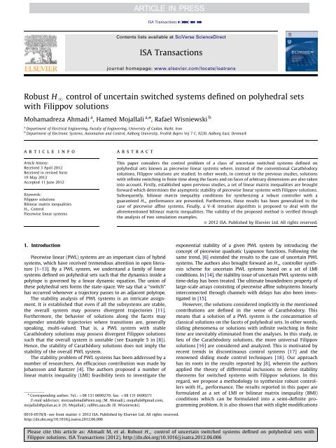
Robust HN control of uncertain switched systems defined on polyhedral sets 

with Filippov solutions 

Mohamadreza Ahmadi a , Hamed Mojallali a,n , Rafael Wisniewski b 

a Department of Electrical Engineering, Faculty of Engineering, University of Guilan, Rasht, Iran 

b Department of Electronic Systems, Automation and Control, Aalborg University, Fredrik Bajers Vej 7 C, 9220, Aalborg East, Denmark 

article info 

Article history: 

Received 3 April 2012 

Received in revised form 

19 May 2012 

Accepted 11 June 2012 

Keywords: 

Filippov solutions 

Bilinear matrix inequalities 

H1 Control 

Piecewise linear systems 

1. Introduction 

abstract 

Piecewise linear (PWL) systems are an important class of hybrid 

systems, which have received tremendous attention in open literature 

[1–13]. By a PWL system, we understand a family of linear 

systems defined on polyhedral sets such that the dynamics inside a 

polytope is governed by a linear dynamic equation. The union of 

these polyhedral sets forms the state-space. We say that a ‘‘switch’’ 

has occurred whenever a trajectory passes to an adjacent polytope. 

The stability analysis of PWL systems is an intricate assignment. 

It is established that even if all the subsystems are stable, 

the overall system may possess divergent trajectories [11]. 

Furthermore, the behavior of solutions along the facets may 

engender unstable trajectories where transitions are, generally 

speaking, multi-valued. That is, a PWL system with stable 

Carathéodory solutions may possess divergent Filippov solutions 

such that the overall system is unstable (see Example 5 in [8]). 

Hence, the stability of Carathédory solutions does not imply the 

stability of the overall PWL system. 

The stability problem of PWL systems has been addressed by a 

number of researchers. An efficacious contribution was made by 

Johansson and Rantzer [4]. The authors proposed a number of 

linear matrix inequality (LMI) feasibility tests to investigate the 

n Corresponding author. Tel.: þ98 131 6690270; fax: þ98 131 6690271 

E-mail addresses: mrezaahmadi@ieee.org (M. Ahmadi), mojallali@gmail.com, 

mojallali@guilan.ac.ir (H. Mojallali), raf@es.aau.dk (R. Wisniewski). 

ISA Transactions ] (]]]]) ]]]–]]] 

Contents lists available at SciVerse ScienceDirect 

ISA Transactions 

journal homepage: www.elsevier.com/locate/isatrans 

0019-0578/$ - see front matter & 2012 ISA. Published by Elsevier Ltd. All rights reserved. 

http://dx.doi.org/10.1016/j.isatra.2012.06.006 

This paper considers the control problem of a class of uncertain switched systems defined on 

polyhedral sets known as piecewise linear systems where, instead of the conventional Carathéodory 

solutions, Filippov solutions are studied. In other words, in contrast to the previous studies, solutions 

with infinite switching in finite time along the facets and on faces of arbitrary dimensions are also taken 

into account. Firstly, established upon previous studies, a set of linear matrix inequalities are brought 

forward which determines the asymptotic stability of piecewise linear systems with Filippov solutions. 

Subsequently, bilinear matrix inequality conditions for synthesizing a robust controller with a 

guaranteed H1 performance are presented. Furthermore, these results has been generalized to the 

case of piecewise affine systems. Finally, a V–K iteration algorithm is proposed to deal with the 

aforementioned bilinear matrix inequalities. The validity of the proposed method is verified through 

the analysis of two simulation examples. 

& 2012 ISA. Published by Elsevier Ltd. All rights reserved. 

exponential stability of a given PWL system by introducing the 

concept of piecewise quadratic Lyapunov functions. Following the 

same trend, [6] extended the results to the case of uncertain PWL 

systems. The authors also brought forward an H1 controller synthesis 

scheme for uncertain PWL systems based on a set of LMI 

conditions. In [14], the stability issue of uncertain PWL systems with 

time-delay has been treated. The ultimate boundedness property of 

large-scale arrays consisting of piecewise affine subsystems linearly 

interconnected through channels with delays has also been investigated 

in [15]. 

However, the solutions considered implicitly in the mentioned 

contributions are defined in the sense of Carathéodory. This 

means that a solution of a PWL system is the concatenation of 

classical solutions on the facets of polyhedral sets. In other words, 

sliding phenomena or solutions with infinite switching in finite 

time are inevitably eliminated from the analyses. In this study, in 

lieu of the Carathéodory solutions, the more universal Filippov 

solutions [16] are considered and analyzed. This is motivated by 

recent trends in discontinuous control systems [17] and the 

renowned sliding mode control techniques [18]. Our approach 

has its roots in the results reported by [8], wherein the authors 

applied the theory of differential inclusions to derive stability 

theorems for switched systems with Filippov solutions. In this 

regard, we propose a methodology to synthesize robust controllers 

with H1 performance. The results reported in this paper are 

formulated as a set of LMI or bilinear matrix inequality (BMI) 

conditions which can be formulated into a semi-definite programming 

problem. It is also shown that with slight modifications 

Please cite this article as: Ahmadi M, et al. Robust H N control of uncertain switched systems defined on polyhedral sets with 

Filippov solutions. ISA Transactions (2012), http://dx.doi.org/10.1016/j.isatra.2012.06.006

2 

the same results can be utilized to analyze piecewise affine (PWA) 

systems. 

The framework of this paper is organized as follows. A brief 

introduction to polyhedral sets and the notations used in this 

paper are presented in the subsequent section. The stability 

problem of PWL systems is addressed in Section 3. The H1 

Controller synthesis methodology and a V–K iteration algorithm to 

deal with the BMI conditions are described in Section 4. The 

accuracy of the proposed method is evaluated by two simulation 

examples in Section 5. The paper ends with conclusions in Section 6. 

2. Notations and definitions 

A polyhedral set is defined by finitely many linear inequalities 

fxAR n 9Exkeg with EAR s n and eAR s where the notation k 

signifies the component-wise inequality. This definition connotes 

that a polyhedra is the intersection of a finite number of halfspaces. 

A polytope is a bounded polyhedral set or equivalently the 

convex hull of finitely many points. Suppose X be a polyhedral set 

and assume H be a halfspace such that X H. Let X F ¼ X \ H be 

non-empty. Then, the polyhedron X F is called a (proper) face of X. 

Obviously, the improper faces of X are the subsets | and X. Faces 

of dimension dimðXÞ 1 are called facets [19]. 

In this study, we will consider a class of switched systems with 

Filippov solutions S ¼fX,U,V,X,I,F,Gg, where X R n is a polyhedral 

set representing the state space, X ¼fXigiA I is the set 

containing the polytopes in X with index set I ¼f1; 2, ...,nXg 

(note that S 

i A IX i ¼ X). Each polytope Xi is characterized by the 

set fxAX9E ixk0g. U is the control space and V is the disturbance 

space, which are both subsets of Euclidean spaces. In addition, 

each function v(t) belongs to the class of square integrable 

functions L2½0,1Þ; i.e., the class of functions for which 

JvJL 2 ¼ 

Z 1 

0 

vðtÞ T vðtÞ dt 

1=2 

is well-defined and finite. F ¼ffigi A I and G ¼fgigiA I are families of 

linear functions associated with the system states x and outputs y. 

Each fi consists of six elements ðAi,Bi,D i; DAi,DBi,DD iÞ and each gi is 

composed of four elements ðCi,Gi; DCi,DGiÞ. Furthermore, 

f i : Yi U V-R n ; ðx,u,vÞ/fzAR n 9z ¼ðAiþDAiÞxþðBiþDB iÞuþ ðDi þ 

DDiÞvg and gi : Yi U-R m ; ðx,uÞ/fzAR m 9z ¼ðCiþDC iÞxþ ðGiþ DGiÞug where Yi is an open neighborhood of Xi. The set of matrices 

ðAi,Bi,C i,Di,G iÞ are defined over the polytope Xi and (DAi,DBi, DCi, DDi,DGi) encompass the corresponding uncertainty terms. In 

order to derive the stability and control results, we assume that 

the upper bound of uncertainties are known apriori; i.e., 

DA T 

i DA i rA T 

i A i 

DB T 

i DB i rB T 

i B i 

DC T 

i DC i rC T 

i C i 

DD T 

i DD i rD T i D i 

DG T 

i DGi rG T 

i Gi ð1Þ 

in which ðAi,Bi,C i,Di,G iÞ are any set of constant matrices with the 

same dimension as ðAi,Bi,C i,Di,G iÞ satisfying (1). 

The dynamics of the system can be described by 

_xðtÞAcoðF ðxðtÞ,uðtÞ,vðtÞÞÞ ð2Þ 

yðtÞAGðxðtÞ,uðtÞÞ ð3Þ 

M. Ahmadi et al. / ISA Transactions ] (]]]]) ]]]–]]] 

where coð Þ denotes the convex hull, the set valued maps [20] F 

and G are defined as 

F : X U V-2 X ; ðx,u,vÞ/fzAR n 9z ¼ f iðx,u,vÞ if xAX ig ð4Þ 

G : X U-2 Rm 

; ðx,uÞ/fzAR m 9z ¼ giðx,uÞ if xAX ig ð5Þ 

where the notation 2 A means the power set or the set of all 

subsets of A. Denote by ~ I ¼fði,jÞAI 2 9Xi \ Xj a|,iajg the set of 

index pairs which determines the polytopes with non-empty 

intersections. We now assume that each polytope is the intersection 

of a finite set of supporting halfspaces. By Nij denote the 

normal vector pertained to the hyperplane supporting both Xi and 

Xj. Consequently, each boundary can be characterized as 

Xi \ Xj ¼fxAX9N T 

ijx 0, Hijxk0, ði,jÞA ~ Ig ð6Þ 

where represent the component-wise equality and the inequality 

Hijxk0 confines the hyperplane to the interested region. Throughout 

the paper, the matrix inequalities should be understood in the 

sense of positive definiteness; i.e., A4B ðAZBÞ means A B is 

positive definite (semi-positive definite). In case of matrix inequalities, 

I denotes the unity matrix (the size of I can be inferred from the 

context) and should be distinguished from the index set I. In 

matrices, % in place of a matrix entry amn means that amn ¼ aT nm . 

A Filippov solution to (2) is an absolutely continuous function 

½0,TÞ-X; t/fðtÞ ðT40Þ which solves the following Cauchy 

problem 

_fðtÞAcoðF ðfðtÞ,uðtÞ,vðtÞÞÞ a:e:, fð0Þ¼f0 ð7Þ 

In the sequel, it is assumed that at any interior point xAX there 

exists a Filippov solution to system (1). This can be evidenced by 

Proposition 5 in [8]. For more information pertaining to the 

solutions and their existence or uniqueness properties, the interested 

reader is referred to the expository review [21] and the 

didactic book [16]. 

3. Stability of PWL systems with Filippov Solutions 

In [8], a stability theorem for switched systems defined on 

polyhedral sets in the context of Filippov solutions is proposed. In 

what follows, we reformulate this latter stability theorem in terms 

of matrix inequalities which provides computationally doable 

means to inspect the robust stability of uncertain switched systems. 

These matrix inequalities would be later utilized to devise a 

stabilizing controller with H1 disturbance rejection performance. 

Lemma 1. Consider the following autonomous PWL system 

_x AcoðF ðxÞÞ ð8Þ 

with DAi 0. If there exists quadratic forms FiðxÞ¼xTQ ix, CiðxÞ¼ xTðA T 

i Q i þQ iAiÞx and CijðxÞ¼xTðA T 

j Q i þQ iAjÞx satisfying 

F iðxÞ40 for all xAX i\f0g ð9Þ 

CiðxÞo0 for all xAX i\f0g ð10Þ 

for all iAI, and 

C ijðxÞo0 for all xAX i \ X j\f0g ð11Þ 

F iðxÞ¼F jðxÞ for all xAX i \ X j ð12Þ 

for all ði,jÞA ~ I. Then, the equilibrium point 0 of (8) is asymptotically 

stable. 

Remark 1. The inclusions xAX i\f0g and xAX i \ X j are analogous 

to fxAX9E ixg0g and (6), respectively. 

It is worth noting that Conditions (9)–(10) are concerned with 

the positivity of a quadratic form over a polytope; whereas, (11) is 



about positivity over a hyperplane. Condition (12) asserts that the 

candidate Lyapunov functions should be continuous (along the 

facets). A well known LMI formulation of conditions (9), (10) and 

(12) was proposed in [4] which is described next. Let us construct 

a set of matrices F i, iAI such that F ix ¼ F jx for all xAX i \ X j and 

ði,jÞA ~ I. Then, it follows that the piecewise linear candidate 

Lyapunov functions can be formulated as 

VðxÞ¼x T F T 

i MFix ¼ x T Q ix if xAX i ð13Þ 

where the free parameters of Lyapunov functions are concentrated 

in the symmetric matrix M. In the following lemma we 

generalize the results proposed by [4] to PWL systems with the 

more general Filippov solutions. 

Lemma 2. Consider the PWL system (8) with Fillipov solutions, and 

the family of piecewise quadratic Lyapunov functions ViðxÞ¼xT Q ix ¼ xTF T 

i MFix, iAI. If there exist a set of symmetric matrices Qi, three sets of symmetric matrices Ui, Si, Tij with non-negative entries, 

and matrices Wij of appropriate dimensions with iAI and ði,jÞA ~ I, 

such that the following LMI problem is feasible 

Q i E T 

i S iE i 40 ð14Þ 

A T 

i Q i þQ iAi þE T 

i UiEi o0 ð15Þ 


A T 

j Q i þQ iA j þW ijN T 

ij þN ijW T 

ij þHT 

ij T ijH ij o0 ð16Þ 

for all ði,jÞA ~ I. Then, the equilibrium point 0 of (8) is asymptotically 

stable. 

Proof. Matrix inequalities (14) and (15) are the same as Eq. (11) 

in Theorem 1 in [4] which satisfy (9)–(10). The continuity of the 

Lyapunov functions is also ensured from the assumption that 

V iðxÞ¼xTQ ix ¼ xTF T 

i MFix , iAI since Fix ¼ Fjx, for all xAX i \ Xj and 

ði,jÞA ~ I. (11) is equivalent to xTðA T 

j Q i þQ iAjÞxo0 for fxAX9N T 

ijx 0, 

Hijxg0g. Applying the S-procedure and Finsler’s lemma [22], we 

obtain (16) for a set of matrices Tij, ði,jÞA ~ I with non-negative 

entries and Wij, ði,jÞA ~ I with appropriate dimensions. & 

We remark that algorithms for constructing matrices Ei and Fi, 

iAI, are described in [9]. 

Remark 2. A similar LMI formulation to (11) can be found in [9]; 

whereas, our analysis, in this paper, is established upon the 

stability theorem delineated in Proposition 10 in [8] which 

considered the Filippov Solutions. 

4. Robust controller synthesis with H1 performance 

In this section, we propose a set of conditions to design a 

robust stabilizing switching controller of the form 

uAKðxÞ 

K : X-2 U ; x/fzAU9z ¼ K ix if xAX ig ð17Þ 

with a guaranteed H1 performance [23]. That is, a controller such 

that, in addition to asymptotic stability (limt-1fðtÞ¼0 for all 

FðtÞ satisfying (7)), ensures that the induced L 2-norm of the 

operator from v(t) to the controller output y(t) is less than a 

constant Z40 under zero initial conditions ðxð0Þ¼0Þ; in other 

words, 

JyJL rZJvJL 2 2 

given any non-zero vAL2½0,1Þ. 

M. Ahmadi et al. / ISA Transactions ] (]]]]) ]]]–]]] 3 

ð18Þ 

If we apply the switching controller (17) to (2) and (3), we 

arrive at the following controlled system with outputs 

_xðtÞAcoð ~F ðxðtÞ,vðtÞÞÞ 

yðtÞA ~ GðxðtÞÞ ð19Þ 

where ~F : X V-2 X ; ðx,vÞ/fzAR n 9z ¼ A cixþD civ if xAX ig and 

G : X-2 Rm 

; x/fzAR m 9z ¼ C ciðxÞ if xAX ig with 

A ci ¼ A i þDA i þðB i þDB iÞK i 

D ci ¼ D i þDD i 

C ci ¼ C i þDC i þðG i þDG iÞK i 

ð20Þ 

Theorem 1. System (19) is asymptotically stable at the origin with 

disturbance attenuation Z as defined in (18), if there exist a set of 

symmetric matrices Q i, iAI, three sets of symmetric matrices U i, S i, 

iAI , Tij, ði,jÞA ~ I with non-negative entries, and matrices Wij, ði,jÞA ~ I 

of appropriate dimensions such that 

Q i E T 


A T 

ci Q i þQ iA ci þE T 

i U iE i þZ 2 Q iD ciD T 

ci Q i þC T 

ci C ci o0 ð22Þ 


A T 

cjQ i þQ iAcj þW ijN T 

ij þNijW T 

ij þHTijT 

ijHij þZ 2 Q iDcjD T 

cjQ i þC T 

cjCcj o0 

for all ði,jÞA ~ I. 

Proof. Refer to Appendix A. 

ð23Þ 

Theorem 2. Given a constant Z40, the closed loop control system 

(19) is asymptotically stable at the origin with disturbance attenuation 

Z, if there exist constants E ij 40, ði,jÞA ~ I, E i 40, iAI, matrices K i, 

iAI, a set of symmetric matrices Qi, iAI, three sets of symmetric 

matrices U i, S i, iAI , T ij, ði,jÞAI with non-negative entries, and 

matrices Wij, ði,jÞA ~ I of appropriate dimensions such that 

Q i E T 


L i o0 ð25Þ 


L ij o0 ð26Þ 

for all ði,jÞA ~ I, where 

L i ¼ 

2 

6 

4 

Pi Q i K T 

i BTi 

K T 

i BTi 

K T 

i GTi 

K T 

i GTi 

% Y 1 

i 0 0 0 0 

Ei % % 

1þE 2 I 0 0 0 

i 

% % % 

1 

I 0 0 

E i 

% % % % 

E i 

2þE i þE 2 i 

% % % % % 

I 0 

E i 

1þE i þ2E 2 i 


Filippov solutions. ISA Transactions (2012), http://dx.doi.org/10.1016/j.isatra.2012.06.006 

3 

7 

I 5

4 

L ij ¼ 

with 

2 

6 

4 

Pij Q i K T 

j BTj 

K T 

j BTj 

K T 

j GT 

j 

K T 

j GTj 

% Y 1 

ij 0 0 0 0 

Eij % % 

1þE 2 I 0 0 0 

ij 

% % % 

1 

I 0 0 

E ij 

% % % % 

Eij 2þE ij þE2 ij 

% % % % % 

P i ¼ A T 

i Q i þQ iA i þE T 

i U iE i þE iA T 

i A i þ 1þ 3 

E i 

I 0 

P ij ¼ A T 

j Q i þQ iA j þW ijN T 

ij þN ijW T 

ij þHT 

ij T ijH ij þE ijA T 

j A j 

þ 1þ 3 

E ij 

Y i ¼ E i þ 3 

E i 

and 

Y ij ¼ E ij þ 3 

E ij 

C T 

j C j þð1þ3E ijÞC T 

j C j 

IþZ 2 1þ 1 

E i 

IþZ 2 1þ 1 

E ij 

D iD T 

i þZ 2 ð1þE iÞD iD T i 

D jD T 

j þZ 2 ð1þE ijÞD jD T j 

Eij 1þE ij þ2E2 ij 

3 

7 

I 5 

C T 

i C i þð1þ3E iÞC T 

i C i 

Proof. We need to apply Theorem 1. Inequality (24) corresponds 

to (21). Substituting (27) in (23), the left-hand side of (23) is 

simplified as LHS ¼ðAjþDAj þðBjþDBjÞKjÞ T Q i þ Q iðAj þDAj þðBjþ DBjÞK jÞþWijN T 

ij þNijW T 

ij þHTijT 

ijHij þZ 2Q iðDj þDDjÞðDj þ DDjÞ T Q i þ 

ðCj þDC j þðGiþDGiÞK jÞ T ðCj þDC j þðGiþDGiÞK jÞrA T 

j Q i þQ iAj þW ij 

N T 

ij þNijW T 

ij þHTijT 

ijHij þK T 

j BTj 

Q i þQ iBjK j þ 2=EijQ iQ i þEijA T 

j Aj þ EijK T 

j 

B T 

j B jK j þ Z 2 Q iðð1þ1=E ijÞD jD T 

j þð1þE ijÞD jD T j ÞQ i þ ð1þE ijÞC T 

j C j þ 

ð1þE ijÞC T 

j Cj þ1=EijC T 

j Cj þEijK T 

j GTj 

GjK j þ1=EijC T 

j Cj þEijK T 

j GTj 

GjK j þEijC T 

j 

Cj þ1=EijK T 

j GTj 

GjK j þEijC T 

j Cj þ 1=EijK T 

j GTj 

GjK j þK T 

j ðð1þ1=E ijÞG T 

j Gj þð1þ 

EijÞG T 

j GjÞK j. 

With some calculation, it can be verified that 

LHSrP ij þQ i 

2 

IþZ 

Eij 2 1þ 1 

Eij ! 

þE ijK T 

j BT 

j B jK j þ 2þE ij þE 2 ij 

E ij 

D T 

j D j þZ 2 ð1þE ijÞD jD T j Q i 

K T 

j GT 

j G jK j þ 1þE ij þ2E 2 ij 

E ij 

þ 1 

K 

Eij T 

j BTj 

BjK j þEijQ iQ i þ 1 

Q 

E 

iQ i þEijK ij 

T 

j BTj 

BjK j 

! 

K T 

j GT 

j G jK j 

which is equivalent to LHSrP ij þQ iYijQ i þ ðð1þE2 ijÞ=EijÞ K T 

j BT 

j 

BjK j þEijK T 

j BTj 

BjK j þðð2þEij þE2 ijÞ=EijÞK T 

j GTj 

GjK j þðð1þEij þ2E2 ijÞ=EijÞK T 

j 

G T 

j G jK j. 

Utilizing Shur complement theorem, (26) can be obtained. Thus, 

if (26) is feasible, then (23) is satisfied. Analogously, it can be 

proved that (25) is consistent with (22). & 

Remark 3. The conditions derived in Theorem 2 are BMIs [24] 

in the variables Qi and Ki. 

In order to deal with the BMI conditions encountered in 

Theorem 2, the following V–K iteration algorithm [25] is suggested: 

Initialization: Select a set of controller gains based on pole 

placement method or any other controller design scheme to 

predetermine a set of initial controller gains. 


Step V: Given the set of fixed controller gains Ki, iAI, solve the 

following optimization problem 

min gi Q i,Si,U i,T ij 

subject to ð24Þ,Li giIo0 and Lij giIo0 for a set of matrices Qi, iAI. 

Step K: Given the set of fixed controller gains Qi, iAI, solve the 

following optimization problem 

min gi Ki,S i,U i,T ij 

subject to ð24Þ,Li giIo0 and Lij giIo0 for a set of matrices Ki, iAI. 

The algorithm continues till g i o0, iAI. 

Remark 4. Generalization of the results presented in this paper 

to the case of piecewise affine (PWA) dynamics is straightforward. 

This can be simply realized by augmenting the corresponding 

system matrices as demonstrated in [8]. The interested reader can 

refer to Appendix B. 

5. Simulation results 

In this section, we demonstrate the performance of the 

proposed approach using numerical examples. Example 1 deals 

with a switched system with Filippov solutions which is asymptotically 

stable at the origin; but, the disturbance attenuation 

performance is not satisfactory. Unlike Example 1, Example 

2 considers an unstable PWL system in which both asymptotic 

stability and disturbance mitigation are investigated based on the 

proposed approach. Not to mention that in both cases uncertainties 

are also associated with the nominal systems. 

5.1. Example 1 

Suppose the state-space X ¼ R 2 is divided into four polytopes 

corresponding to the four quadrants of the second dimensional 

Euclidean space; i.e, 

X1 ¼fðx1,x2ÞAR 2 9x1 40 and x2 40g 

X2 ¼fðx1,x2ÞAR 2 9x1 o0 and x2 40g 

X3 ¼fðx1,x2ÞAR 2 9x1 o0 and x2 o0g 

X 4 ¼fðx 1,x 2ÞAR 2 9x 1 40 and x 2 o0g ð27Þ 

Consider a PWL system with Filippov solutions characterized by 

(19) and (20) where the associated system matrices are given by 

A1 ¼ A3 ¼ 

0 1 

2 0 , A2 ¼ A4 ¼ 

B1 ¼ B2 ¼ B3 ¼ B4 ¼ 1 

0 

C1 ¼ C2 ¼ C3 ¼ C4 ¼ 2 

0 

D1 ¼ D2 ¼ D3 ¼ D4 ¼ 0 

0:1 

T 

T 

0 1 

0:5 0 

and the uncertainty bounds specified as 

A1 ¼ A3 ¼ 

0 0:03 

0:03 0 

, A2 ¼ A4 ¼ 

0:03 0 

0 0:03 



C1 ¼ C3 ¼ 0:01 

0 

T 

, C2 ¼ C4 ¼ 

0 

0:01 

The matrices regarding the polytopes can be constructed as 

E1 ¼ E3 ¼ 

F1 ¼ E1 

I 

1 0 

0 1 , E2 ¼ E4 ¼ 

, F2 ¼ E2 

I 

, F3 ¼ E3 

I 

N 12 ¼ N 34 ¼ 1 

0 , N 14 ¼ N 23 ¼ 0 

1 

H 12 ¼ H 34 ¼ 

T 

1 0 

0 1 

0 1 

0 0 , H 14 ¼ H 23 ¼ 

, F4 ¼ E4 

I 

1 0 

0 0 

Based on Theorem 2, a switching controller as defined in (17) is 

designed in order to ensure that (in addition to preserving the 

asymptotic stability property of the system) under zero initial 

conditions the disturbance signal of vðtÞ¼5 cosðptÞ is attenuated 

with Z ¼ 0:05. In this experiment, the constant scalars were preset 

to E12 ¼ E23 ¼ E14 ¼ E34 ¼ 1 and E1 ¼ E2 ¼ E3 ¼ E4 ¼ 5. The algorithm 

was initialized using pole placement method with initial pole 

positions of ð 1, 2Þ and controller gains of 

K1 ¼ K3 ¼ 

3 

0 

T 

, K2 ¼ K4 ¼ 

The following solutions was obtained in two iterations 

Q 1 ¼ Q 3 ¼ 

K1 ¼ K3 ¼ 

78:29 5:96 

5:96 3:01 , Q 2 ¼ Q 4 ¼ 

0:9014 

0:8292 

g min ¼ 7:03921 10 4 

3 

5 

T 

, K2 ¼ K4 ¼ 

T 

33:06 1:35 

1:35 65:14 

0:1137 

0:2715 

Fig. 1 sketches the trajectories of the closed-loop system 

without disturbance when the H1 controller is incorporated. This 

demonstrates that the Filippov solutions of the closed-loop 

system are asymptotically stable at 0. One should observe that 

the solutions entering the facet x2 ¼ 0 cannot leave the facet (the 

so called attractive sliding mode property). This is due to the fact 

that the velocities at both regions X 1 and X 2 are toward the facet. 

x 2 

4 

3 

2 

1 

0 

−1 

−2 

−3 

−4 

−4 −3 −2 −1 0 

x1 1 2 3 4 

Fig. 1. The trajectories of the closed loop system. The dashed lines illustrate the 

facets. 

T 


0.5 

0 

−0.5 

−1 

−1.5 

−2 

−2.5 

−3 

0 10 20 30 40 50 60 

1.2 

1 

0.8 

0.6 

0.4 

0.2 

0 

−0.2 

0 10 20 30 40 50 60 

Fig. 2. Evolution of system states when the H1 controller is applied: with an 

initial condition on a non-attractive facet (top) and with an initial condition on an 

attractive facet (bottom). 

We emphasize that this result could not been achieved by 

previous studies which excluded those solutions with infinite 

switching in finite time. Moreover, Fig. 2. displays the evolution of 

the states of the closed-loop system. The applied control inputs 

corresponding to simulations portrayed in Fig. 2 are available in 

Fig. 3. As can be inspected from Fig. 3 (and of course as expected), 

the control signals are discontinuous since switching occurs in the 

neighborhood of the attractive facets. This switching in the 

applied control signals diminishes considerably as the trajectories 

converge to origin in approximately 30 s. 

The disturbance mitigation performance of the proposed 

method can also be deduced from Fig. 4. It can be discerned from 

the figure that the disturbance signal is considerably extenuated 

as the H1 controller is employed. 

5.2. Example 2 

For the sake of comparison, the example used in [6] is 

selected; but, instead of Carathéodory solutions, Filippov solutions 

are investigated. Therefore, the system structure has to be 

modified as delineated next. Consider an uncertain PWL system 

described by (19) and (20) with I ¼f1; 2,3; 4g and the state-space 

is a polyhedral set divided into four polytopes. The associated 



x1 x2 x1 x2

6 

system matrices are 

A1 ¼ A3 ¼ 

Control Input (u) 

Control input (u) 

1 0:1 

0:5 1 , A2 ¼ A4 ¼ 

B1 ¼ B3 ¼ 0 

1 , B2 ¼ B4 ¼ 1 

0 

3 

2.5 

2 

1.5 

1 

0.5 

0 

0 10 20 30 40 50 60 

20 

15 

10 

5 

0 

x 10−3 

−5 

10 15 20 25 30 35 

1 0:5 

0:1 1 

D1 ¼ D2 ¼ D3 ¼ D4 ¼ 0 

1 , C1 ¼ C2 ¼ C3 ¼ C4 ¼ 0 

1 

T 

Control Input (u) 


0.1 

0 

−0.1 

−0.2 

−0.3 

−0.4 

−0.5 

−0.6 

−0.7 

−0.8 

−0.9 

−1 

0 10 20 30 40 50 60 

−10 

10 15 20 25 30 35 

Fig. 3. Time histories of the applied control inputs corresponding to state evolutions provided in Fig. 2 (top), and the same figures enlarged (bottom). 

y 

0.2 

0.15 

0.1 

0.05 

0 

−0.05 

−0.1 

−0.15 

−0.2 

−0.25 

−0.3 

0 5 10 15 20 25 

Time (seconds) 


2 

0 

−2 

−4 

−6 

−8 

The uncertainty bounds are characterized as 

A1 ¼ A3 ¼ 

B1 ¼ B3 ¼ 

x 10−3 

−0.3 

0 5 10 15 20 25 

Time (seconds) 

Fig. 4. Response of the closed loop control system with disturbance and zero initial condition: before applying the H1 controller (left) and after utilizing the H1 controller 

(right). 

y 

0.2 

0.15 

0.1 

0.05 

0 

−0.05 

−0.1 

−0.15 

−0.2 

−0.25 

0 0:02 

0:01 0 

, A2 ¼ A4 ¼ 

0 

0:02 , B2 ¼ B4 ¼ 0:02 

0 

0:01 0 

0 0:02 

The matrices characterizing the polytopes are given as follows 

E1 ¼ E3 ¼ 

1 1 

1 1 , E2 ¼ E4 ¼ 



1 1 

1 1

F1 ¼ E1 

I 

, F2 ¼ E2 

I 

, F3 ¼ E3 

I 

N12 ¼ N34 ¼ 1 

1 , N14 ¼ N23 ¼ 

H12 ¼ H34 ¼ 

1 

1 

1 0 

1 0 , H14 ¼ H23 ¼ 

, F4 ¼ E4 

I 

1 0 

1 0 

It is worth noting that the open-loop system is unstable and since 

solutions with infinite switching in finite time are present the 

approach reported in [6] and common Lyapunov based methods 

are not applicable. The V–K iteration algorithm is initialized using 

pole placement method. The assigned closed-loop poles for the 

dynamics in each polytope are ð 3, 2Þ and the corresponding 

initial controller gains are 

K1 ¼ K3 ¼ 

119:5 

7 

T 

, K2 ¼ K4 ¼ 

5 

19:5 

Using the scheme presented in this paper for a set of constants 

E12 ¼ E23 ¼ E14 ¼ E34 ¼ 10 and E1 ¼ E2 ¼ E3 ¼ E4 ¼ 100, the following 

x 2 

x 2 

4 

3 

2 

1 

0 

−1 

−2 

−3 

−4 

−4 −3 −2 −1 0 

x1 1 2 3 4 

4 

3 

2 

1 

0 

−1 

−2 

−3 

−4 

−4 −3 −2 −1 0 

x1 1 2 3 4 

Fig. 5. The trajectories of the closed loop control system. H1 synthesis based on 

[6] (top), and using the proposed methodology (bottom). The dashed lines 

illustrate the facets. 

T 


solutions has been obtained 

Q 1 ¼ Q 3 ¼ 

K 1 ¼ K 3 ¼ 

463:75 24:94 

24:94 2:39 , Q 2 ¼ Q 4 ¼ 

637:72 

30:14 

g min ¼ 2:7186 10 5 

T 

, K 2 ¼ K 4 ¼ 

21:53 

1:69 

52:26 7:39 

7:39 763:47 

for the H1 controller design with Z ¼ 0:1 infiveiterations.Consequently, 

it follows from Theorem 2 that the closed loop control 

system is asymptotically stable at the origin and the disturbance 

attenuation criterion is satisfied. Fig. 5. demonstrates the simulation 

results of four different initial conditions (in the absence of 

disturbance) using both the method expounded in [6] and the 

suggested scheme which prove the stability of the closed loop 

systems. It can be examined that the approach in [6] neglects the 

sliding motion along the facets; hence, it cannot take into account the 

solutions with infinite switching in finite time which are intrinsic to 

switched systems. Notice, in particular, that solutions with infinite 

switching in finite time on facets are also present (see Fig. 6.) when 

the proposed method is exploited. Additionally, the applied control 

inputs associated with the simulations in Fig. 6 are shown in Fig. 7. 

Once again as expected, the controller starts to switch (discontinuous 

1 

0.5 

0 

−0.5 

−1 

−1.5 

0 50 100 150 

3 

2.5 

2 

1.5 

1 

0.5 

0 

0 50 100 150 

Fig. 6. Evolution of system states when the H1 controller is applied: with an 

initial condition in the interior of a polytope (top) and with an initial condition on 

an attractive facet (bottom). 



T 

x1 x2 x1 x2

8 



behavior) when the trajectories reach an attractive facet. The fluctuations 

of the control signal mitigates significantly in around 130 s, 

implying that the solutions have converged to the origin. This should 

be opposed to the results in [6] where only Carathódory solutions 

are taken into account. Additionally, the simulation results in the 

presence of disturbance (vðtÞ¼4sinð2ptÞ) and zero initial conditions 

are illustrated in Fig. 8, which ascertains the disturbance attenuation 

performance of the proposed controller. 

6. Conclusions 

6 

5 

4 

3 

2 

1 

0 

0 50 100 150 

2 

1.8 

1.6 

1.4 

1.2 

1 

0.8 

0.6 

0.4 

0.2 

x 10−3 

0 

90 100 110 120 130 140 150 

In this paper, the stability and control problem of uncertain PWL 

systems with Filippov Solutions was considered. The foremost 


2 

0 

−2 

−4 

−6 

−8 

−10 

−12 

−14 

−16 

0 50 100 150 

−2 

90 100 110 120 130 140 150 

Fig. 7. Time histories of the applied control inputs corresponding to state evolutions provided in Fig. 6 (top), and the same figures enlarged (bottom). 

Controlled output y 

0.04 

0.03 

0.02 

0.01 

0 

−0.01 

−0.02 

−0.03 

−0.04 

0 1 2 3 4 5 



Controlled output y 

1 

0.5 

0 

−0.5 

−1 

−1.5 

0.04 

0.03 

0.02 

0.01 

−0.01 

−0.02 

−0.03 

x 10−3 

0 

−0.04 

0 1 2 3 4 5 

Fig. 8. Response of the closed loop control system with disturbance and zero initial condition: the stable controller synthesis (left) and the H1 controller synthesis (right). 

purpose of this research was to extend the previous results on 

switched systems defined on polyhedral sets to the case of solutions 

with infinite switching in finite time and sliding motions. In this 

regard, a set of matrix inequality conditions are brought forward to 

investigate the stability of a PWL system in the framework of 

Filippov solutions. Additionally, a method based on BMIs are devised 

for the synthesis of stable and robust H1 controllers for uncertain 

PWL systems with Filippov solutions. These schemes has been 

examined through simulation experiments. The following subjects 

are suggested for further research: 

Due to practical considerations, it is sometimes desirable to 

assuage the switching frequency in the control signal which 

may contribute to unwanted outcomes, e.g., high heat losses in 



power circuits, mechanical wear, and etc. The authors suggest 

the application of chattering-free techniques such as boundary 

layer control (BLC). However, how these methods could be 

embedded in the framework of the analyses presented here is 

still an open problem. 

The robust control and stability results can be extended to 

other solution types for discontinuous systems, e.g. Krasovskii, 

Aizerman and Gantmakher (see the expository review [21]). 

The curious reader may consult [26] for novel (robust) stability 

analysis results on nonlinear switched systems defined on 

compact sets in the context of Filippov solutions. 

Appendix A. Proof of Theorem 1 

From (21)–(22) and Lemma 2, it can be discerned that the 

Filippov solutions of the closed loop system (19) converge to 0 

asymptotically. Additionally, since Q i ¼ F T 

i MFi and Fix ¼ Fjx, for all 

xAX i \ Xj the continuity of the Lyapunov functions is assured. 

What remains is to show that the disturbance attenuation 

performance is Z. Define a multi-valued function 

UðxÞ¼fzAR9z ¼ V iðxÞ if xAX ig ðA:1Þ 

and set GðxÞ¼coðUðxÞÞ. This can be thought of as a switched 

Lyapunov function. Differentiating and integrating G with respect 

to t yields 

Z 1 

0 

þ 

dG 

dt ¼ 

dt 

Z t2 

t 1 

aj j ¼ 1 

þ Xr 

bj j ¼ 1 

Z 1 

þ Xm 

þ 

Z t1 

0 

½x T ðA T 

c1 Q 1 þQ 1Ac1Þxþv T D T 

c1 Q 1xþx T Q 1Dc1vŠ dt þ 

½x T ðA T 

c2 Q 2 þQ 2Ac2Þxþv T D T 

c2 Q 2xþx T Q 2Dc2vŠ dt þ 

Z tk 

t k 1 

Z tl 

t l 1 

½x T ðA T 

cjQ k þQ kAcjÞxþv T D T 

cjQ kxþx T o 

Q kDcjvŠ dt þ 

½x T ðA T 

cjQ l þQ lAcjÞxþv T D T 

cjQ lxþx T o 

Q lDcjvŠ dt þ 

½x T ðA T 

cn Q n þQ nAcnÞxþv T D T 

cn Q nxþx T Q nDcnvŠ dt 

tn 

wherein aj, bj 40 such that Pn j ¼ 1 aj ¼ 1, and Pn j ¼ 1 bj ¼ 1. m and r 

are the number of neighboring cells to a boundary where the 

solutions possess infinite switching in finite time (in the time 

intervals of ½tk 1,t kŠ and ½tl 1,tlŠ), respectively. With the above 

formulation, we consider a state evolution scenario including the 

interior of different polytopes as well as the facets. Suppose 

conditions (22) and (23) hold, then it follows that 

Z b 

a 

½x T ðA T 

ci Q i þQ iA ciÞxþv T D T 

ci Q ixþx T Q iD civŠ dt 

o 

r 

r 

Z b 

a 

þv T D T 

Z b 

a 

Z b 

a 

½x T ð E T 

i U iE i Z 2 Q iD ciD T 

ci Q i C T 

ci C ciÞx 

ci Q ixþx T Q iD civþZ 2 v T v Z 2 v T vŠ dt 

½ y T yþZ 2 v T v Z 2 ðv Z 2 D T 

ci Q ixÞ T ðv Z 2 D T 

ci Q ixÞÞŠ dt 

ð y T yþZ 2 v T vÞ dt 

Correspondingly, 

Xn Z d 

aj ½x 

j ¼ 1 c 

T ðA T 

cjQ ( 

i þQ iAcjÞx þv T D T 

cjQ ixþx T ) 

Q iDcjvŠ dt 

o Xn 

Z d 

aj ½x T ð WijN T 

ij NijW T 

ij HTijT 

( 

ijHij j ¼ 1 

c 


r 

r 

Z 2 Q iD cjD T 

cj Q i C T 

cj C cjÞxþZ 2 v T v Z 2 v T vŠ dt 

0 

Z d 

y 

c 

T yþZ 2 v T v Xn 

ajðZ j ¼ 1 

2 ðv Z 2 D T 

cjQ ixÞ T 

@ ðv Z 2 D T 

Z d 

c 


) 

1 

cjQ ixÞÞAdt 

where, a,b,c,d40 are arbitrary non-negative constants (b4a, and 

d4c). Finally, we arrive at the justification that 

Z 1 Z t1 

dG 

dt r ð y 

dt T yþZ 2 v T Z t2 

vÞ dtþ ð y T yþZ 2 v T vÞ dt þ 

0 

0 

Z tk 

þ 

t k 1 

Z tl 

þ 

þ 

tl 1 

Z 1 

which reduces to 

tn 

Gðxð1ÞÞ Gðxð0ÞÞr 

ð y T yþZ 2 v T vÞ dt þ 

ð y T yþZ 2 v T vÞ dt þ 


Z 1 

0 

t 1 

ð y T yþZ 2 v T vÞ dt ðA:2Þ 

Moreover, note that xð1Þ ¼ xð0Þ¼0. This can be concluded from 

the assumption on zero initial conditions, and from the fact that 

the system is asymptotically stable at origin (as demonstrated 

earlier in this proof). Consequently, we have 

0r 

Z 1 

0 

ð y T yþZ 2 v T vÞ dt ðA:3Þ 

which is equivalent to (18). This completes the proof. 

Appendix B. Generalization to piecewise affine systems 

It is worth noting that all results obtained for PWL systems 

with Filippov solutions can also be accommodated for PWA 

systems. However, the following modifications should be applied 

in advance. 

Consider a PWA system with Filippov solutions S ¼fX ,U, V, 

X,I,F,Gg, where X DR n þ 1 is a polyhedral set representing the 

state space, X ¼fXigi A I is the set containing the polytopes in X 

with index set I ¼f1; 2, ...,nXg (note that S 

i A IX i ¼ X ). F ¼ffigi A I 

and G ¼fgigi A I are families of linear functions associated with the 

(augmented) system states x ¼½xT 1Š T AX and outputs y. Each f i 

consists of six elements ðAi,B i,D i; DAi,DB i,DD iÞ and each gi is 

composed of four elements ðCi,G i; DCi,DG iÞ. 

The following augmented system matrices can be constructed 

Ai ¼ Ai 0 

ai 0 , Bi ¼ Bi 0 , Di ¼ Di 0 , Ci ¼½Ci 0Š ðB:1Þ 

where ai is the affine term associated with the dynamics in 

the polytope Xi, and correspondingly the augmented uncertain 

matrices 

DA i ¼ DA i Da i 

0 0 

, DB i ¼ DB i 

0 

DDi ¼ DDi , DCi ¼½DCi 0Š ðB:2Þ 

0 

Besides, the matrices characterizing each polytope can also be 

modified as 

E i ¼½E i e iŠ and F i ¼½F i f iŠ ðB:3Þ 



,

10 

Then, each polytope is defined as 

X i ¼fx AX 9E ixk0g ðB:4Þ 

and for all x AX i \ X j and ði,jÞA ~ I it holds that 

F ix ¼ F jx ðB:5Þ 

Hence, the candidate Lyapunov function in effect in the polytope 

Xi is formulated as 

V iðxÞ¼x T T 

Fi M Fix ¼ x T Q ix ðB:6Þ 

It is possible that the facets may not have intersections at the 

origin. Therefore, let 

" # 

N ij ¼ N ij 

n ij 

and H ij ¼ H ij h ij 

0 0 

ðB:7Þ 

and each boundary can be characterized as 

Xi \ Xj ¼fxAX 9N T 

ijx 0, Hijxk0, ði,jÞA ~ Ig ðB:8Þ 

With the above formulation at hand, one can utilize the results 

given in this paper for PWA systems. This is simply accomplished 

by replacing the associated matrices for PWL systems by their 

PWA counterparts. 

References 

[1] de Best J, Bukkems B, van de Molengraft M, Heemels W. Robust control of 

piecewise linear systems: a case study in sheet flow control. Control 

Engineering Practice 2008;16:991–1003. 

[2] Azuma S, Yanagisawa E, Imura J. Controllability analysis of biosystems based 

on piecewise affine systems approach. IEEE Transactions on Automatic 

Control, Special Issue on Systems Biology 2008;139–159. 

[3] Balochian S, Sedigh AK. Sufficient conditions for stabilization of linear time 

invariant fractional order switched systems and variable structure control 

stabilizers. ISA Transactions 2012;51:65–73. 

[4] Johansson M, Rantzer A. Computation of piecewise quadratic lyapunov functions 

for hybrid systems. IEEE Transactions on Automatic Control 1998;43(2): 

555–9. 

[5] Goncalves J, Megretski A, Dahleh MA. Global analysis of piecewise linear 

systems using impact maps and surface lyapunov functions. IEEE Transactions 

on Automatic Control 2003;48(12):2089–106. 


[6] Chan M, Zhu C, Feng G. Linear-matrix-inequality-based approach to H1 

controller synthesis of uncertain continuous-time piecewise linear systems. 

IEE Proceedings–Control Theory and Applications 2004;151(3):295–301. 

[7] Ohta Y, Yokoyama H. Stability analysis of uncertain piecewise linear systems 

using piecewise quadratic lyapunov functions. In: IEEE international symposium 

on intelligent control; 2010. p. 2112–2117. 

[8] Leth J, Wisniewski R. On formalism and stability of switched systems. Journal 

of Control Theory and Applications 2012;10(2):176–83. 

[9] Johansson M. Piecewise linear control systems. Berlin: Springer-Verlag; 2003. 

[10] Sun Z. Stability of piecewise linear systems revisited. Annual Reviews in 

Control 2010;34:221–31. 

[11] Branicky M. Multiple lyapunov functions and other analysis tools for switched 

and hybrid systems. IEEE Transactions on Automatic Control 1998;43(4): 

475–82. 

[12] Hassibi A, Boyd S. Quadratic stabilization and control of piecewise-linear 

systems. In: American control conference, vol. 6; 1998. p. 3659–3664. 

[13] Singh H, Sukavanam N. Simulation and stability analysis of neural network based 

control scheme for switched linear systems. ISA Transactions 2012;51:105–10. 

[14] K. Moezzi, L. Rodrigues, A. Aghdam, Stability of uncertain piecewise affine 

systems with time-delay. In: American control conference; 2009. p. 2373– 

2378. 

[15] Kashima K, Papachristodoulou A, Algöer F. A linear multi-agent systems 

approach to diffusively coupled piecewise affine systems: delay robustness. 

In: Joint 50th IEEE conference on decision and control and European control 

conference; 2010. p. 603–608. 

[16] Filippov A. Differential equations with discontinuous right-hand sides. 

Mathematics and its applications Soviet Series, vol. 18. Dordrecht: Kluwer 

Academic Publishers Group; 1988. 

[17] Boiko I. Discontinuous control systems. Boston: Birkhäuser; 2009. 

[18] Edwards C, Colet E, Fridman L, editors. Advances in variable structure and 

sliding mode control. Lecture Notes in Control and Information Science. 

Berlin: Springer; 2006. 

[19] Grunbaum B. Convex polytopes. 2 ed.Springer-Verlag; 2003. 

[20] Aubin J, Cellina A. Differential Inclusions: Set-Valued Maps And Viability 

Theory, vol. 264, Grundl. der Math. Wiss. Berlin, Springer-Verlag; 1984. 

[21] Cortes J. Discontinuous dynamical systems: a tutorial on solutions, nonsmooth 

analysis, and stability. IEEE Control Systems Magazine 1998;28(3): 

36–73. 

[22] Polik I, Terlaky T. A survey of the S-lemma. SIAM Review 2007;49(3): 

371–418. 

[23] Dullerud G, Paganini F. A course in robust control theory. Springer; 2000. 

[24] Antwerp JV, Braatz R. A toturial on linear and bilinear matrix inequalities. 

Journal of Process Control 2000;10:363–85. 

[25] Banjerdpongchai D, How J. Parametric robust H1 controller synthesis: 

comparison and convergence analysis. In: American control conference; 

1998. p. 2403–2404. 

[26] Ahmadi M, Mojallali H, Wisniewski R, Izadi-Zamanabadi R. Robust stability 

analysis of nonlinear switched systems with Filippov solutions. In: 7’th IFAC 

symposium on robust control design. Aalborg, Denmark; 2012.

ISA Transactions - VBN

You also want an ePaper? Increase the reach of your titles

Delete template?

Save as template?