Bayesian Nonparametric Learning of Markov Switching Processes
Bayesian Nonparametric Learning of Markov Switching Processes
Bayesian Nonparametric Learning of Markov Switching Processes

You also want an ePaper? Increase the reach of your titles
YUMPU automatically turns print PDFs into web optimized ePapers that Google loves.
[ Emily B. Fox, Erik B. Sudderth, Michael I. Jordan, and Alan S. Willsky ]<br />
[ Stochastic process priors<br />
for dynamical systems]<br />
<strong>Markov</strong> switching processes,<br />
such as the<br />
hidden <strong>Markov</strong> model<br />
(HMM) and switching<br />
linear dynamical system<br />
(SLDS), are <strong>of</strong>ten used to describe<br />
rich dynamical phenomena. They<br />
describe complex behavior via repeated<br />
returns to a set <strong>of</strong> simpler models:<br />
imagine a person alternating between<br />
walking, running, and jumping behaviors,<br />
or a stock index switching<br />
between regimes <strong>of</strong> high and low volatility.<br />
Classical approaches to identification<br />
and estimation <strong>of</strong> these models<br />
assume a fixed, prespecified number <strong>of</strong><br />
dynamical models. We instead examine<br />
<strong>Bayesian</strong> nonparametric approaches<br />
that define a prior on <strong>Markov</strong><br />
switching processes with an unbounded<br />
number <strong>of</strong> potential model parameters (i.e., <strong>Markov</strong><br />
modes). By leveraging stochastic processes such as the beta<br />
and Dirichlet process (DP), these methods allow the data to<br />
drive the complexity <strong>of</strong> the learned model, while still permitting<br />
efficient inference algorithms. They also lead to generalizations<br />
that discover and model dynamical behaviors shared<br />
among multiple related time series.<br />
Digital Object Identifier 10.1109/MSP.2010.937999<br />
INTRODUCTION<br />
A core problem in statistical signal processing<br />
is the partitioning <strong>of</strong> temporal<br />
data into segments, each <strong>of</strong> which permits<br />
a relatively simple statistical<br />
description. This segmentation problem<br />
arises in a variety <strong>of</strong> applications, in<br />
areas as diverse as speech recognition,<br />
computational biology, natural language<br />
processing, finance, and cryptanalysis.<br />
While in some cases the problem is<br />
merely that <strong>of</strong> detecting temporal<br />
changes (in which case the problem can<br />
be viewed as one <strong>of</strong> changepoint detection),<br />
in many other cases the temporal<br />
segments have a natural meaning in the<br />
domain and the problem is to recognize<br />
recurrence <strong>of</strong> a meaningful entity (e.g., a<br />
© PHOTODISC<br />
particular speaker, a gene, a part <strong>of</strong><br />
speech, or a market condition). This<br />
leads naturally to state-space models, where the entities that are<br />
to be detected are encoded in the state.<br />
The classical example <strong>of</strong> a state-space model for segmentation<br />
is the HMM [1]. The HMM is based on a discrete state variable<br />
and on the probabilistic assertions that the state transitions<br />
are <strong>Markov</strong>ian and that the observations are conditionally independent<br />
given the state. In this model, temporal segments are<br />
equated with states, a natural assumption in some problems but<br />
a limiting assumption in many others. Consider, for example,<br />
the dance <strong>of</strong> a honey bee as it switches between a set <strong>of</strong> turn<br />
1053-5888/10/$26.00©2010IEEE<br />
IEEE SIGNAL PROCESSING MAGAZINE [43] NOVEMBER 2010
ight, turn left, and waggle dances.<br />
It is natural to view these<br />
dances as the temporal segments,<br />
as they “permit a relatively simple<br />
statistical description.” But<br />
each dance is not a set <strong>of</strong> conditionally<br />
independent draws from a fixed distribution as required<br />
by the HMM—there are additional dynamics to account for.<br />
Moreover, it is natural to model these dynamics using continuous<br />
variables. These desiderata can be accommodated within the<br />
richer framework <strong>of</strong> <strong>Markov</strong> switching processes, specific examples<br />
<strong>of</strong> which include the switching vector autoregressive (VAR)<br />
process and the SLDS. These models distinguish between the<br />
discrete component <strong>of</strong> the state, which is referred to as a<br />
“mode,” and the continuous component <strong>of</strong> the state, which captures<br />
the continuous dynamics associated with each mode.<br />
These models have become increasingly prominent in applications<br />
in recent years [2]–[8].<br />
While <strong>Markov</strong> switching processes address one key limitation<br />
<strong>of</strong> the HMM, they inherit various other limitations <strong>of</strong> the<br />
HMM. In particular, the discrete component <strong>of</strong> the state in the<br />
<strong>Markov</strong> switching process has no topological structure<br />
(beyond the trivial discrete topology). Thus it is not easy to<br />
z 1 z 2 z 3 z 4<br />
. . . z n<br />
y 1 y 2 y 3 y 4<br />
. . . y n<br />
(a)<br />
z 1 z 2 z 3 z 4 . . . z n<br />
y 1 y 2 y 3 y 4<br />
. . . y n<br />
(b)<br />
z 1 z 2 z 3 z . . .<br />
4 z n<br />
x 1 x 2 x 3 x 4<br />
. . . x n<br />
. . .<br />
y 1 y 2 y 3 y 4 y n<br />
(c)<br />
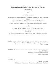
[FIG1] Graphical representations <strong>of</strong> three <strong>Markov</strong> switching<br />
processes: (a) HMM, (b) order 2 switching VAR process, and<br />
(c) SLDS. For all models, a discrete-valued <strong>Markov</strong> process z t<br />
K<br />
evolves as z t11 |5p k<br />
6 k51 , z t = p zt<br />
.For the HMM, observations are<br />
K<br />
generated as y t |5u k<br />
6 k51 , z t = F1u zt<br />
2, whereas the switching<br />
1z<br />
VAR(2) process assumes y t = N1A 2 t 1z<br />
1 y t21 1 A 2 t 2 y t22 , S 1z 2 t<br />
2. The<br />
SLDS instead relies on a latent, continuous-valued <strong>Markov</strong><br />
state x t to capture the history <strong>of</strong> the dynamical process as<br />
specified in (15).<br />
WE NEED TO MOVE BEYOND THE<br />
SIMPLE DISCRETE MARKOV CHAIN<br />
AS A DESCRIPTION OF TEMPORAL<br />
SEGMENTATION.<br />
compare state spaces <strong>of</strong> different<br />
cardinality and it is not possible<br />
to use the state space to<br />
encode a notion <strong>of</strong> similarity<br />
between modes. More broadly,<br />
many problems involve a collection<br />
<strong>of</strong> state-space models (either HMMs or <strong>Markov</strong> switching<br />
processes), and within the classical framework there is no<br />
natural way to talk about overlap between models. A particular<br />
instance <strong>of</strong> this problem arises when there are multiple<br />
time series, and where we wish to use overlapping subsets <strong>of</strong><br />
the modes to describe the different time series. In the section<br />
“Multiple Related Time Series,” we discuss a concrete example<br />
<strong>of</strong> this problem where the time series are motion-capture videos<br />
<strong>of</strong> humans engaging in exercise routines, and where the<br />
modes are specific exercises, such as “jumping jacks” or<br />
“squats.” We aim to capture the notion that two different people<br />
can engage in the same exercise (e.g., jumping jacks) during<br />
their routine.<br />
To address these problems, we need to move beyond the<br />
simple discrete <strong>Markov</strong> chain as a description <strong>of</strong> temporal segmentation.<br />
In this article, we describe a richer class <strong>of</strong> stochastic<br />
processes known as combinatorial stochastic<br />
processes that provide a useful foundation for the design <strong>of</strong><br />
flexible models for temporal segmentation. Combinatorial stochastic<br />
processes have been studied for several decades in<br />
probability theory (see, e.g., [9]), and they have begun to play<br />
a role in statistics as well, most notably in the area <strong>of</strong> <strong>Bayesian</strong><br />
nonparametric statistics where they yield <strong>Bayesian</strong> approaches<br />
to clustering and survival analysis (see, e.g., [10]). The work<br />
that we present here extends these efforts into the time-series<br />
domain. As we aim to show, there is a natural interplay<br />
between combinatorial stochastic processes and state-space<br />
descriptions <strong>of</strong> dynamical systems.<br />
Our primary focus is on two specific stochastic processes—<br />
the DP and the beta process—and their role in describing<br />
modes in dynamical systems. The DP provides a simple description<br />
<strong>of</strong> a clustering process where the number <strong>of</strong> clusters is not<br />
fixed a priori. Suitably extended to a hierarchical DP (HDP),<br />
this stochastic process provides a foundation for the design <strong>of</strong><br />
state-space models in which the number <strong>of</strong> modes is random<br />
and inferred from the data. In the section “Hidden <strong>Markov</strong><br />
Models,” we discuss the HDP and its connection to the HMM.<br />
Building on this connection, the section “<strong>Markov</strong> Jump Linear<br />
Systems” shows how the HDP can be used in the context <strong>of</strong><br />
<strong>Markov</strong> switching processes with conditionally linear dynamical<br />
modes. Finally, in the section “Multiple Related Time Series,”<br />
we discuss the beta process and show how it can be used to capture<br />
notions <strong>of</strong> similarity among sets <strong>of</strong> modes in modeling<br />
multiple time series.<br />
HIDDEN MARKOV MODELS<br />
The HMM generates a sequence <strong>of</strong> latent modes via a discretevalued<br />
<strong>Markov</strong> chain [1]. Conditioned on this mode sequence,<br />
the model assumes that the observations, which may be<br />
IEEE SIGNAL PROCESSING MAGAZINE [44] NOVEMBER 2010
discrete or continuous valued,<br />
are independent. The HMM is<br />
the most basic example <strong>of</strong> a<br />
<strong>Markov</strong> switching process and<br />
forms the building block for<br />
more complicated processes<br />
examined later.<br />
THERE IS A NATURAL INTERPLAY<br />
BETWEEN COMBINATORIAL STOCHASTIC<br />
PROCESSES AND STATE-SPACE<br />
DESCRIPTIONS OF DYNAMICAL SYSTEMS.<br />
parameter space U. Depending<br />
on the form <strong>of</strong> the emission<br />
distribution, various choices <strong>of</strong><br />
H lead to computational efficiencies<br />
via conjugate analysis.<br />
FINITE HMM<br />
Let z t denote the mode <strong>of</strong> the <strong>Markov</strong> chain at time t, and p j<br />
the mode-specific transition distribution for mode j. Given the<br />
mode z t , the observation y t is conditionally independent <strong>of</strong><br />
the observations and modes at other time steps. The generative<br />
process can be described as<br />
z t<br />
0 z t21 | p zt21<br />
y t<br />
0 z t | F1u zt<br />
2 (1)<br />
for an indexed family <strong>of</strong> distributions F1# 2 (e.g., multinomial for<br />
discrete data or multivariate Gaussian for real, vector-valued<br />
data), where u i are the emission parameters for mode i. The<br />
notation x | F indicates that the random variable x is drawn<br />
from a distribution F. We use bar notation x | F | F to specify<br />
conditioned-upon random elements, such as a random distribution.<br />
The directed graphical model associated with the HMM<br />
is shown in Figure 1(a).<br />
One can equivalently represent the HMM via a set <strong>of</strong> transition<br />
probability measures G j 5g K k51 p jk d uk<br />
, where d u is a unit<br />
mass concentrated at u. Instead <strong>of</strong> employing transition distributions<br />
on the set <strong>of</strong> integers (i.e., modes) that index into the<br />
collection <strong>of</strong> emission parameters, we operate directly in the<br />
parameter space U, and transition between emission parameters<br />
with probabilities 5G j<br />
6. Specifically, let j t21 be the unique emission<br />
parameter index j such that ur t21 5u j . Then,<br />
Mode<br />
G 1<br />
G 2<br />
1<br />
2<br />
3<br />
.<br />
.<br />
.<br />
K<br />
Time<br />
1 2 3<br />
θ 1 θ 1 θ 1 θ 1 θ 1<br />
θ 2 θ 2 θ 2 θ 2 θ 2<br />
θ 3 θ 3 θ 3 θ 3 θ 3<br />
.<br />
.<br />
.<br />
π 11<br />
π 21<br />
π 12<br />
.<br />
.<br />
.<br />
θ k θ k θ k θ k θ k<br />
π 13<br />
π 22<br />
π 23<br />
(a)<br />
.<br />
.<br />
.<br />
. . .<br />
.<br />
.<br />
.<br />
π 1K<br />
θ 1 θ 2 θ 3 . . . θ k<br />
π 2K<br />
θ 1 θ 2 θ 3<br />
. . . θ k<br />
T<br />
.<br />
.<br />
.<br />
Θ<br />
Θ<br />
0<br />
0<br />
ur t ur t21 | G jt21<br />
y t ur t | F1ur t<br />
2. (2)<br />
G 3<br />
π 31<br />
π 32<br />
π33<br />
π 3K<br />
Here, u t r [ 5u 1 , c, u K<br />
6 takes the place <strong>of</strong> u zt<br />
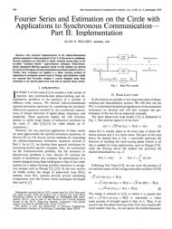
in (1). A visualization<br />
<strong>of</strong> this process is shown by the trellis diagram <strong>of</strong> Figure 2.<br />
One can consider a <strong>Bayesian</strong> HMM by treating the transition<br />
probability measures G j as random, and endowing them<br />
with a prior. Formally, a random measure on a measurable<br />
space U, with sigma algebra A, is defined as a stochastic<br />
process whose index set is A. That is, G1A2 is a nonnegative<br />
random variable for each A [ A. Since the probability measures<br />
are solely distinguished by their weights on the shared<br />
set <strong>of</strong> emission parameters 5u 1 , c, u K<br />
6, we consider a prior<br />
that independently handles these components. Specifically,<br />
take the weights p j 5 3p j1 cp jK<br />
4 (i.e., transition distributions)<br />
to be independent draws from a K -dimensional<br />
Dirichlet distribution,<br />
p j | Dir1a 1 , c, a K<br />
2 j 5 1, c, K, (3)<br />
implying that g k p jk 5 1, as desired. Then, assume that the<br />
atoms are drawn as u j | H for some base measure H on the<br />
=<br />
θ 1 θ 2 θ 3 . . . θ k<br />
(b)<br />
θ ′ 1 θ ′ 2 θ ′ . . . .<br />
3 θ ′ T<br />
θ 2 θ 1 θ 3<br />
=<br />
=<br />
y 1 y 2 y 3 y T<br />
(c)<br />
[FIG2] (a) Trellis representation <strong>of</strong> an HMM. Each circle<br />
represents one <strong>of</strong> the K possible HMM emission parameters at<br />
various time steps. The highlighted circles indicate the selected<br />
emission parameter ur t at time t, and the arrows represent the<br />
set <strong>of</strong> possible transitions from that HMM mode to each <strong>of</strong> the<br />
K possible next modes. The weights <strong>of</strong> these arrows indicate<br />
the relative probability <strong>of</strong> the transitions encoded by the<br />
mode-specific transition probability measures G j . (b) Transition<br />
probability measures G 1 , G 2 , and G 3 corresponding to the<br />
example trellis diagram. (c) A representation <strong>of</strong> the HMM<br />
observations y t , which are drawn from emission distributions<br />
parameterized by the highlighted nodes.<br />
Θ<br />
IEEE SIGNAL PROCESSING MAGAZINE [45] NOVEMBER 2010
This implies the following predictive distribution on the indicator<br />
assignment variables<br />
.<br />
β 5<br />
β 4<br />
β 3<br />
β 2<br />
β 1<br />
p1z N11 5 z|z 1 , c, z N ,g2 5<br />
g d1z, K 1 12<br />
N 1 g<br />
1 1 K<br />
N 1g a n k d1z, k2. (7)<br />
k51<br />
[FIG3] Pictorial representation <strong>of</strong> the stick-breaking construction<br />
<strong>of</strong> the DP.<br />
STICKY HDP-HMM<br />
In the <strong>Bayesian</strong> HMM <strong>of</strong> the previous section, we assumed that<br />
the number <strong>of</strong> HMM modes K is known. But what if this is not<br />
the case? For example, in the<br />
speaker diarization task considered<br />
later, determining the<br />
number <strong>of</strong> speakers involved in<br />
the meeting is one <strong>of</strong> the primary<br />
inference goals. Moreover,<br />
even when a model adequately<br />
describes previous observations,<br />
it can be desirable to allow new modes to be added as more data<br />
are observed. For example, what if more speakers enter the<br />
meeting? To avoid restrictions on the size <strong>of</strong> the mode space,<br />
such scenarios naturally lead to priors on probability measures<br />
G j that have an unbounded collection <strong>of</strong> support points u k .<br />
The DP, denoted by DP1g, H2, provides a distribution over<br />
countably infinite probability measures<br />
G 0 5 àk51<br />
b k d uk<br />
u k | H (4)<br />
on a parameter space U. The weights are sampled via a stickbreaking<br />
construction [11]<br />
k21<br />
b k 5n k q 112n ,<br />
2 n k | Beta11, g2. (5)<br />
,51<br />
In effect, we have divided a unit-length stick into lengths given<br />
by the weights b k : the kth weight is a random proportion v k <strong>of</strong><br />
the remaining stick after the first 1k212 weights have been chosen.<br />
We denote this distribution by b | GEM1g2. See Figure 3<br />
for a pictorial representation <strong>of</strong> this process.<br />
The DP has proven useful in many applications due to its<br />
clustering properties, which are clearly seen by examining the<br />
predictive distribution <strong>of</strong> draws ur i | G 0 . Because probability<br />
measures drawn from a DP are discrete, there is a strictly positive<br />
probability <strong>of</strong> multiple observations ur i taking identical<br />
values within the set 5u k<br />
6, with u k defined as in (4). For each<br />
value ur i , let z i be an indicator random variable that picks out<br />
the unique value u k such that ur i 5u zi<br />
. Blackwell and MacQueen<br />
[12] derived a Pólya urn representation <strong>of</strong> the ur i<br />
i21<br />
g<br />
ur i<br />
0 ur 1 , c, ur i 21 |<br />
g 1 i 2 1 H 1 1<br />
a g1i21 d ur j<br />
j51<br />
K<br />
g<br />
|<br />
g 1 i 2 1 H 1 a<br />
THE HMM IS THE MOST BASIC<br />
EXAMPLE OF A MARKOV SWITCHING<br />
PROCESS AND FORMS THE BUILDING<br />
BLOCK FOR MORE COMPLICATED<br />
PROCESSES EXAMINED LATER.<br />
k51<br />
n k<br />
g 1 i 2 1 d u k<br />
. (6)<br />
Here, n k 5 g N i51 d1z i , k2 is the number <strong>of</strong> indicator random<br />
variables taking the value k, and K11 is a previously unseen<br />
value. The discrete Kronecker delta d1z, k2 5 1 if z 5 k, and 0<br />
otherwise. The distribution on partitions induced by the<br />
sequence <strong>of</strong> conditional distributions in (7) is commonly<br />
referred to as the Chinese restaurant process. Take i to be a<br />
customer entering a restaurant<br />
with infinitely many<br />
tables, each serving a unique<br />
dish u k . Each arriving customer<br />
chooses a table, indicated<br />
by z i , in proportion to how<br />
many customers are currently<br />
sitting at that table. With some<br />
positive probability proportional to g, the customer starts a<br />
new, previously unoccupied table K 1 1. From the Chinese<br />
restaurant process, we see that the DP has a reinforcement<br />
property that leads to a clustering at the values u k . This representation<br />
also provides a means <strong>of</strong> sampling observations<br />
from a DP without explicitly constructing the infinite probability<br />
measure G 0 | DP1g, H2.<br />
One could imagine using the DP to define a prior on the<br />
set <strong>of</strong> HMM transition probability measures G j . Taking each<br />
transition measure G j as an independent draw from DP1g, H2<br />
implies that these probability measures are <strong>of</strong> the form<br />
g `k51 p jk d ujk<br />
, with weights p j | GEM1g2 and atoms u jk | H.<br />
Assuming H is absolutely continuous (e.g., a Gaussian distribution),<br />
this construction leads to transition measures with<br />
nonoverlapping support (i.e., u jk 2 u ,kr with probability one.)<br />
Based on such a construction, we would move from one infinite<br />
collection <strong>of</strong> HMM modes to an entirely new collection<br />
at each transition step, implying that previously visited<br />
modes would never be revisited. This is clearly not what we<br />
intended. Instead, consider the HDP [13], which defines a<br />
collection <strong>of</strong> probability measures 5G j<br />
6 on the same support<br />
points 5u 1 , u 2 , c6 by assuming that each discrete measure<br />
G j is a variation on a global discrete measure G 0 . Specifically,<br />
the <strong>Bayesian</strong> hierarchical specification takes G j | DP1a, G 0<br />
2,<br />
with G 0 itself a draw from a DP1g, H2. Through this construction,<br />
one can show that the probability measures are<br />
described as<br />
`<br />
G 0 5 a b k51<br />
kd uk<br />
G j 5 a<br />
`<br />
k51 p jk d uk<br />
b | g | GEM1g2<br />
p j | a, b | DP1a, b2<br />
u k | H | H.<br />
(8)<br />
Applying the HDP prior to the HMM, we obtain the HDP-HMM<br />
<strong>of</strong> Teh et al. [13].<br />
IEEE SIGNAL PROCESSING MAGAZINE [46] NOVEMBER 2010
Extending the Chinese restaurant<br />
process analogy <strong>of</strong> the DP,<br />
one can examine a Chinese restaurant<br />
franchise that describes<br />
the partitions induced by the HDP.<br />
In the context <strong>of</strong> the HDP-HMM,<br />
the infinite collection <strong>of</strong> emission parameters u k determine a<br />
global menu <strong>of</strong> shared dishes. Each <strong>of</strong> these emission parameters<br />
is also associated with a single, unique restaurant in the<br />
franchise. The HDP-HMM assigns a customer ur t to a restaurant<br />
based on the previous customer ur t21 , since it is this<br />
parameter that determines the distribution <strong>of</strong> u r t [see (2)].<br />
Upon entering the restaurant determined by ur t21 , customer ur t<br />
chooses a table with probability proportional to the current<br />
occupancy, just as in the DP. The dishes for the tables are then<br />
chosen from the global menu G 0 based on their popularity<br />
throughout the entire franchise, and it is through this pooling<br />
<strong>of</strong> dish selections that the HDP induces a shared sparse subset<br />
<strong>of</strong> model parameters.<br />
By defining p j | DP1a, b2, the HDP prior encourages<br />
modes to have similar transition distributions. In particular,<br />
the mode-specific transition distributions are identical<br />
in expectation<br />
A STATE-SPACE MODEL PROVIDES<br />
A GENERAL FRAMEWORK FOR<br />
ANALYZING MANY DYNAMICAL<br />
PHENOMENA.<br />
E3p jk<br />
0 b4 5b k . (9)<br />
Although it is through this construction<br />
that a shared sparse<br />
mode space is induced, we see<br />
from (9) that the HDP-HMM does<br />
not differentiate self-transitions<br />
from moves between different<br />
modes. When modeling data with mode persistence, the flexible<br />
nature <strong>of</strong> the HDP-HMM prior allows for mode sequences<br />
with unrealistically fast dynamics to have large posterior probability,<br />
thus impeding identification <strong>of</strong> a compact dynamical<br />
model which best explains the observations. See an example<br />
mode sequence in Figure 4(a). The HDP-HMM places only a<br />
small prior penalty on creating an extra mode but no penalty<br />
on that mode having a similar emission parameter to another<br />
mode, nor on the time series rapidly switching between two<br />
modes. The increase in likelihood by fine-tuning the parameters<br />
to the data can counteract the prior penalty on creating<br />
this extra mode, leading to significant posterior uncertainty.<br />
These rapid dynamics are unrealistic for many real data sets.<br />
For example, in the speaker diarization task, it is very unlikely<br />
in that two speakers are rapidly switching who is speaking.<br />
Such fast-switching dynamics can harm the predictive performance<br />
<strong>of</strong> the learned model since parameters are informed by<br />
fewer data points. Additionally, in some applications one cares<br />
about the accuracy <strong>of</strong> the inferred label sequence instead <strong>of</strong><br />
Observations<br />
15<br />
10<br />
5<br />
0<br />
−5<br />
Mode<br />
−10<br />
0 200 400 600 800 1,000<br />
Time<br />
11<br />
10<br />
9<br />
8<br />
7<br />
6<br />
5<br />
4<br />
3<br />
2<br />
1<br />
0<br />
0 200 400 600 800 1,000<br />
Time<br />
(a)<br />
Observations<br />
Mode<br />
8<br />
6<br />
4<br />
2<br />
0<br />
−2<br />
−4<br />
−6<br />
−8<br />
0 200 400 600 800 1,000<br />
Time<br />
11<br />
10<br />
9<br />
8<br />
7<br />
6<br />
5<br />
4<br />
3<br />
2<br />
1<br />
0<br />
0 200 400 600 800 1,000<br />
Time<br />
(b)<br />
14<br />
12<br />
10<br />
8<br />
6<br />
4<br />
2<br />
0<br />
−2<br />
−4<br />
0 200 400 600 800 1,000<br />
Time<br />
(c) (d) (e)<br />
Observations<br />
[FIG4] In (a) and (b), mode sequences are drawn from the HDP-HMM and sticky HDP-HMM priors, respectively. In (c)–(e), observation<br />
sequences correspond to draws from a sticky HDP-HMM, an order two HDP-AR-HMM, and an order one BP-AR-HMM with five time<br />
series <strong>of</strong>fset for clarity. The observation sequences are colored by the underlying mode sequences.<br />
IEEE SIGNAL PROCESSING MAGAZINE [47] NOVEMBER 2010
y 1 y 2 y 3<br />
0<br />
p j | a, k, b | DPaa1k, ab1kd ear dynamical process. Just as with the HMM, the switching<br />
j<br />
a1k b. (10) mechanism is based on an underlying discrete-valued <strong>Markov</strong><br />
Here, 1ab1kd j<br />
2 indicates that an amount k .0 is added to<br />
γ<br />
κ<br />
α<br />
β<br />
π κ<br />
the jth component <strong>of</strong> ab. This construction increases the<br />
expected probability <strong>of</strong> self-transition by an amount proportional<br />
to k. Specifically, the expected set <strong>of</strong> weights for transition<br />
distribution p j is a convex combination <strong>of</strong> those defined by b<br />
∞<br />
and mode-specific weight defined by k:<br />
. . . y T<br />
When k50, the original HDP-HMM <strong>of</strong> Teh et al. [13] is recovered.<br />
z 1 z 2 z 3 . . . z T<br />
E3p jk | b, a, k4 5<br />
a<br />
a 1 k b k 1<br />
k<br />
λ θ κ<br />
d1 j, k2.<br />
a 1 k<br />
∞<br />
(11)<br />
(a)<br />
Because positive k values increase the prior probability<br />
E3p jj | b, a, k4 <strong>of</strong> self-transitions, this model is referred to as<br />
γ<br />
κ<br />
β<br />
the sticky HDP-HMM. See the graphical model <strong>of</strong> Figure 5(a)<br />
and the mode sequence sample path <strong>of</strong> Figure 4(b). The k<br />
parameter is reminiscent <strong>of</strong> the self-transition bias parameter<br />
α π κ<br />
<strong>of</strong> the infinite HMM [15], an urn model obtained by integrating<br />
out the random measures in the HDP-HMM. However, that<br />
∞<br />
z 1 z 2 z 3 . . . z T<br />
paper relied on heuristic, approximate inference methods. The<br />
λ θ κ<br />
full connection between the infinite HMM and the HDP, as well<br />
∞<br />
as the development <strong>of</strong> a globally consistent inference algorithm,<br />
was made in [13] but without a treatment <strong>of</strong> a self-tran-<br />
y 1 y 2 y 3<br />
. . . y T<br />
sition parameter. Note that in the formulation <strong>of</strong> Fox et<br />
(b)<br />
al. [14], the HDP concentration parameters a and g, and the<br />
γ<br />
κ<br />
α<br />
λ<br />
β<br />
π κ<br />
θ κ<br />
sticky parameter k, are given priors and are thus learned from<br />
the data as well. The flexibility garnered by incorporating<br />
learning <strong>of</strong> the sticky parameter within a cohesive <strong>Bayesian</strong><br />
framework allows the model to additionally capture fast modeswitching<br />
if such dynamics are present in the data.<br />
∞<br />
z 1 z 2 z 3 . . . z T<br />
In [14], the sticky HDP-HMM was applied to the speaker<br />
diarization task, which involves segmenting an audio recording<br />
∞<br />
into speaker-homogeneous regions, while simultaneously identifying<br />
the number <strong>of</strong> speakers. The data for the experiments<br />
x 1 x 2 x 3<br />
. . . x T<br />
y 1 y 2 y 3<br />
. . . y T<br />
consisted <strong>of</strong> a standard benchmark data set distributed by NIST<br />
as part <strong>of</strong> the Rich Transcription 2004–2007 meeting recognition<br />
(c)<br />
evaluations [16], with the observations taken to be the first<br />
19 Mel frequency cepstral coefficients (MFCCs) computed over<br />
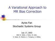
[FIG5] Graphical representations <strong>of</strong> three <strong>Bayesian</strong> nonparametric short, overlapping windows. Because the speaker-specific emissions<br />
are not well approximated by a single Gaussian, a DP<br />
variants <strong>of</strong> the <strong>Markov</strong> switching processes shown in Figure 1.<br />
The plate notation is used to compactly represent replication <strong>of</strong><br />
nodes in the graph [13], with the number <strong>of</strong> replicates indicated mixture <strong>of</strong> Gaussian extension <strong>of</strong> the sticky HDP-HMM was<br />
by the number in the corner <strong>of</strong> the plate. (a) The sticky HDP- considered. The sticky parameter proved pivotal in learning<br />
HMM. The mode evolves as z t11 |5p k<br />
6 k51 , z t = p zt<br />
, where<br />
such multimodal emission distributions. Combining both the<br />
p k | a, k, b = DP1a1k, 1ab 1 kd k<br />
2 / 1a1k22 and b|g =GEM1g2,<br />
and observations are generated as y t |5u k<br />
6 k51 , z t =F1u zt<br />
2. The mode-persistence captured by the sticky HDP-HMM, along<br />
HDP-HMM <strong>of</strong> [13] has k50. (b) A switching VAR (2) process and with a model allowing multimodal emissions, state-<strong>of</strong>-the-art<br />
(c) SLDS, each with a sticky HDP-HMM prior on the <strong>Markov</strong><br />
speaker diarization performance was achieved.<br />
switching process. The dynamical equations are as in (17).<br />
MARKOV JUMP LINEAR SYSTEMS<br />
just doing model averaging. In such applications, one would<br />
like to be able to incorporate prior knowledge that slow,<br />
smoothly varying dynamics are more likely.<br />
To address these issues, Fox et al. [14] proposed to instead<br />
sample transition distributions p j as<br />
The HMM’s assumption <strong>of</strong> conditionally independent observations<br />
is <strong>of</strong>ten insufficient in capturing the temporal dependencies<br />
present in many real data sets. Recall the example <strong>of</strong><br />
the dancing honey bees from the “Introduction” section. In<br />
such cases, one can consider more complex <strong>Markov</strong> switching<br />
processes, namely the class <strong>of</strong> <strong>Markov</strong> jump linear systems<br />
b g | GEM1g2<br />
(MJLSs), in which each dynamical mode is modeled via a lin-<br />
IEEE SIGNAL PROCESSING MAGAZINE [48] NOVEMBER 2010
mode sequence. Switched affine and piecewise affine models,<br />
which we do not consider in this article, instead allow mode<br />
transitions to depend on the continuous state <strong>of</strong> the dynamical<br />
system [17].<br />
STATE-SPACE MODELS, VAR PROCESSES,<br />
AND FINITE MARKOV JUMP LINEAR SYSTEMS<br />
A state-space model provides a general framework for<br />
analyzing many dynamical phenomena. The model consists<br />
<strong>of</strong> an underlying state, x t [ R n , with linear dynamics<br />
observed via y t [ R d . A linear time-invariant state-space<br />
model, in which the dynamics do not depend on time, is<br />
given by<br />
x t 5 Ax t21 1 e t y t 5 Cx t 1 w t , (12)<br />
where e t and w t are independent, zero-mean Gaussian noise<br />
processes with covariances S and R, respectively. The graphical<br />
model for this process is equivalent to that <strong>of</strong> the HMM depicted<br />
in Figure 1(a), replacing z t with x t .<br />
An order r VAR process, denoted by VAR(r), with observations<br />
y t [ R d , can be defined as<br />
y t 5 a<br />
r<br />
i51<br />
A i y t2i 1 e t e t | N10, S2. (13)<br />
Here, the observations depend linearly on the previous r observation<br />
vectors. Every VAR(r) process can be described in statespace<br />
form by, for example, the following transformation:<br />
A 1 A 2 c A r I<br />
I 0 c 0 0<br />
x t 5 ≥<br />
¥ x t21 1 ≥ ¥ e t<br />
( f ( (<br />
(<br />
0 c I 0 0<br />
y t 5 cI 0 c 0d x t . (14)<br />
On the other hand, not every state-space model may be<br />
expressed as a VAR(r) process for finite r [18].<br />
Building on the HMM <strong>of</strong> the section “Finite HMM,” we define<br />
an SLDS by<br />
z t | p zt21<br />
x t 5 A 1z t 2 x t21 1 e t<br />
1z t<br />
2 y t 5 Cx t 1 w t . (15)<br />
Here, we assume the process noise e t<br />
1z t<br />
2 | N10, S 1z 2 t<br />
2 is modespecific,<br />
while the measurement mechanism is not. This assumption<br />
could be modified to allow<br />
for both a mode-specific measurement<br />
matrix C 1z 2 t<br />
and noise w t<br />
1z t<br />
2 |<br />
N10, R 1z 2 t<br />
2. However, such a choice is<br />
not always necessary nor appropriate<br />
for certain applications, and can have Observation dynamics<br />
implications on the identifiability <strong>of</strong><br />
the model. We similarly define a<br />
switching VAR(r) process by<br />
z t | p zt21<br />
y t 5 a<br />
r<br />
i51<br />
A i<br />
1z t 2 y t2i 1 e t<br />
1z t<br />
2. (16)<br />
Both the SLDS and the switching VAR process are contained<br />
within the class <strong>of</strong> MJLS, with graphical model representations<br />
shown in Figure 1(b) and (c). Compare to that <strong>of</strong> the HMM in<br />
Figure 1(a).<br />
HDP-AR-HMM AND HDP-SLDS<br />
In the formulations <strong>of</strong> the MJLS mentioned in the section<br />
“<strong>Markov</strong> Jump Linear Systems,” it was assumed that the number<br />
<strong>of</strong> dynamical modes was known. However, it is <strong>of</strong>ten desirable<br />
to relax this assumption to provide more modeling<br />
flexibility. It has been shown that in such cases, the sticky<br />
HDP-HMM can be extended as a <strong>Bayesian</strong> nonparametric<br />
approach to learning both SLDS and switching VAR processes<br />
[19], [20]. Specifically, the transition distributions are<br />
defined just as in the sticky HDP-HMM. However, instead <strong>of</strong><br />
independent observations, each mode now has conditionally<br />
linear dynamics. The generative processes for the resulting<br />
HDP-AR-HMM and HDP-SLDS are summarized in (17), shown<br />
at the bottom <strong>of</strong> the page, with an example HDP-AR-HMM<br />
observation sequence depicted in Figure 4(d).<br />
Here, p j is as defined in (10). The issue, then, is in determining<br />
an appropriate prior on the dynamic parameters.<br />
In [19], a conjugate matrix-normal inverse-Wishart (MNIW)<br />
prior [21] was proposed for the dynamic parameters 5A 1k2 , S 1k2 6<br />
in the case <strong>of</strong> the HDP-SLDS, and 5A 1k2 1 , c, A 1k2 r , S 1k2 6 for the<br />
HDP-AR-HMM. The HDP-SLDS additionally assumes an<br />
inverse-Wishart prior on the measurement noise R; however,<br />
the measurement matrix, C, is fixed for reasons <strong>of</strong> identifiability.<br />
The MNIW prior assumes knowledge <strong>of</strong> either the autoregressive<br />
order r, or the underlying state dimension n, <strong>of</strong> the<br />
switching VAR process or SLDS, respectively. Alternatively,<br />
Fox et al. [20] explore an automatic relevance determination<br />
(ARD) sparsity-inducing prior [22]–[24] as a means <strong>of</strong> learning<br />
MJLS with variable order structure. The ARD prior penalizes<br />
nonzero components <strong>of</strong> the model through a zero-mean<br />
Gaussian prior with gamma-distributed precision. In the context<br />
<strong>of</strong> the HDP-AR-HMM and HDP-SLDS, a maximal autoregressive<br />
order or SLDS state dimension is assumed. Then, a<br />
structured version <strong>of</strong> the ARD prior is employed so as to drive<br />
1k2<br />
entire VAR lag blocks A i or columns <strong>of</strong> the SLDS matrix A 1k2<br />
to zero, allowing one to infer nondynamical components <strong>of</strong> a<br />
given dynamical mode.<br />
HDP-AR-HMM<br />
HDP-SLDS<br />
Mode dynamics z t | p zt21<br />
z t | p zt21<br />
r<br />
y t 5 a<br />
i51<br />
A i<br />
1z t 2 y t2i 1 e t<br />
1z t<br />
2 x t 5 A 1z t 2 x t21 1 e t<br />
1z t<br />
2<br />
y t 5 Cx t 1 w t<br />
. (17)<br />
IEEE SIGNAL PROCESSING MAGAZINE [49] NOVEMBER 2010
The previous work <strong>of</strong> Fox et al. [8] considered a related,<br />
yet simpler formulation for modeling a maneuvering target<br />
as a fixed LDS driven by a switching exogenous input. Since<br />
the number <strong>of</strong> maneuver modes was assumed unknown, the<br />
exogenous input was taken to be the emissions <strong>of</strong> a HDP-<br />
HMM. This work can be viewed as an extension <strong>of</strong> the work<br />
by Caron et al. [25] in which the exogenous input was an<br />
independent noise process generated from a DP mixture<br />
model. The HDP-SLDS <strong>of</strong> [19] is a departure from these<br />
works since the dynamic parameters themselves change<br />
with the mode, providing a<br />
much more expressive model.<br />
In [19], the utility <strong>of</strong> the<br />
HDP-SLDS and HDP-AR-<br />
HMM was demonstrated on<br />
two different problems: 1)<br />
detecting changes in the volatility<br />
<strong>of</strong> the IBOVESPA stock<br />
index and 2) segmenting<br />
sequences <strong>of</strong> honey bee dances. The dynamics underlying<br />
both <strong>of</strong> these data sets appear to be quite complex, yet can<br />
be described by repeated returns to simpler dynamical models,<br />
and as such have been modeled with <strong>Markov</strong> switching<br />
processes [26], [27]. Without prespecifying domain-specific<br />
knowledge, and instead simply relying on a set <strong>of</strong> observations<br />
along with weakly informative hyperprior settings, the<br />
HDP-SLDS and HDP-AR-HMM were able to discover the<br />
underlying structure <strong>of</strong> the data with performance competitive<br />
with these alternative methods, and consistent with<br />
domain expert analysis.<br />
OUR BAYESIAN NONPARAMETRIC<br />
APPROACH ENVISIONS A LARGE LIBRARY<br />
OF BEHAVIORS, WITH EACH TIME SERIES<br />
OR OBJECT EXHIBITING A SUBSET OF<br />
THESE BEHAVIORS.<br />
MULTIPLE RELATED<br />
TIME SERIES<br />
In many applications, one would like to discover and model<br />
dynamical behaviors which are shared among several related<br />
time series. By jointly modeling such time series, one can<br />
improve parameter estimates, especially in the case <strong>of</strong> limited<br />
data, and find interesting structure in the relationships between<br />
the time series. Assuming that each <strong>of</strong> these time series is modeled<br />
via a <strong>Markov</strong> switching process, our <strong>Bayesian</strong> nonparametric<br />
approach envisions a large library <strong>of</strong> behaviors, with each<br />
time series or object exhibiting a subset <strong>of</strong> these behaviors. We<br />
aim to allow flexibility in the number <strong>of</strong> total and sequencespecific<br />
behaviors, while encouraging objects to share similar subsets<br />
<strong>of</strong> the behavior library. Additionally, a key aspect <strong>of</strong> a flexible<br />
model for relating time series is to allow the objects to switch<br />
between behaviors in different manners (e.g., even if two people<br />
both exhibit running and walking behaviors, they might alternate<br />
between these dynamical modes at different frequencies).<br />
One could imagine a <strong>Bayesian</strong> nonparametric approach<br />
based on tying together multiple time series under the HDP<br />
prior outlined in the section “Sticky HDP-HMM.” However,<br />
such a formulation assumes that all time series share the same<br />
set <strong>of</strong> behaviors, and switch among them in exactly the same<br />
manner. Alternatively, Fox et al. [28] consider a featural representation,<br />
and show the utility <strong>of</strong> an alternative family <strong>of</strong> priors<br />
based on the beta process [29], [30].<br />
FINITE FEATURE MODELS OF<br />
MARKOV SWITCHING PROCESSES<br />
Assume we have a finite collection <strong>of</strong> behaviors 5u 1 , c, u K<br />
6<br />
that are shared in an unknown manner among N objects. One<br />
can represent the set <strong>of</strong> behaviors each object exhibits via an<br />
associated list <strong>of</strong> features. A standard featural representation for<br />
describing the N objects employs an N 3 K binary matrix<br />
F 5 5f ik<br />
6. Setting f ik 5 1 implies<br />
that object i exhibits feature k<br />
for some t [ 51, c, T i<br />
6, where<br />
T i is the length <strong>of</strong> the ith time<br />
series. To discover the structure<br />
<strong>of</strong> behavior sharing (i.e., the<br />
feature matrix), one takes the<br />
feature vector f i 5 3f i1 , c, f iK<br />
4<br />
to be random. Assuming each<br />
feature is treated independently, this necessitates defining a feature<br />
inclusion probability v k for each feature k. Within a<br />
<strong>Bayesian</strong> framework, these probabilities are given a prior that is<br />
then informed by the data to provide a posterior distribution on<br />
feature inclusion probabilities. For example, one could consider<br />
the finite <strong>Bayesian</strong> feature model <strong>of</strong> [31] that assumes<br />
v k | Betaa a K , 1b<br />
f ik | v k | Bernoulli1v k<br />
2. (18)<br />
Beta random variables v k [ 10, 12, and can thus be thought <strong>of</strong><br />
as defining coin-tossing probabilities. The resulting biased coin<br />
is then tossed to define whether f ik is 0 or 1 (i.e., the outcome <strong>of</strong><br />
a Bernoulli trial). Because each feature is generated independently,<br />
and a Beta1a, b2 random variable has mean a/ 1a 1 b2,<br />
the expected number <strong>of</strong> active features in an N 3 K matrix is<br />
Na / 1a/K 1 12 , Na.<br />
A hierarchical <strong>Bayesian</strong> featural model also requires priors<br />
for behavior parameters u k , and the process by which each<br />
object switches among its selected behaviors. In the case <strong>of</strong><br />
<strong>Markov</strong> switching processes, this switching mechanism is governed<br />
by the transition distributions <strong>of</strong> object i, p 1i2 j . As an<br />
example <strong>of</strong> such a model, imagine that each <strong>of</strong> the N objects is<br />
described by a switching VAR process (see the section “<strong>Markov</strong><br />
Jump Linear Systems”) that moves among some subset <strong>of</strong> K<br />
possible dynamical modes. Each <strong>of</strong> the VAR process parameters<br />
u k 5 5A k , S k<br />
6 describes a unique behavior. The feature vector f i<br />
constrains the transitions <strong>of</strong> object i to solely be between the<br />
selected subset <strong>of</strong> the K possible VAR processes by forcing<br />
p 1i2 jk 5 0 for all k such that f ik 5 0. One natural construction<br />
places Dirichlet priors on the transition distributions, and some<br />
prior H (e.g., an MNIW) on the behavior parameters. Then,<br />
p j 1i2 | f i , g, k | Dir1 3g, c, g, g1k, g, c, g4 # f i<br />
2 u k | H,<br />
(19)<br />
IEEE SIGNAL PROCESSING MAGAZINE [50] NOVEMBER 2010
where # denotes the element-wise, or Hadamard, vector product.<br />
Let y 1i2 t represent the observation vector <strong>of</strong> the ith object at<br />
1i2<br />
time t, and z t the latent behavior mode. Assuming an order r<br />
switching VAR process, the dynamics <strong>of</strong> the ith object are<br />
described by the following generative process:<br />
z 1i2 1i2<br />
t | z t21<br />
1i2<br />
| p<br />
1i2 zt21<br />
y t 1i2 5 a<br />
r<br />
j51<br />
(20)<br />
1i2<br />
A 1i2 j, zt<br />
y t2j 1 e 1i2 t<br />
1z 1i2 t<br />
2 ! A<br />
1i2| zt y 1i2 t 1 e 1i2 t<br />
1z 1i2 t<br />
2, (21)<br />
with c . 0, gives rise to completely random measures<br />
G | GP1c, G 0<br />
2, where GP denotes a gamma process. Normalizing<br />
G yields draws from a DP1a, G 0 /a2, with a5G 0<br />
1U2. Random<br />
probability measures G are necessarily not completely random<br />
since the random variables G1A 1<br />
2 and G1A 2<br />
2 for disjoint sets A 1<br />
and A 2 are dependent due to the normalization constraint.<br />
Now consider a rate measure defined as the product <strong>of</strong> a base<br />
measure B 0 , with total mass B 0<br />
1U2 5a, and an improper beta<br />
distribution on the product space U z 30, 14<br />
1i2 5<br />
where e 1i2 t<br />
1k2 | N10, S k<br />
2, A k 5 3A 1, k c A r, k<br />
4, and | y t<br />
1i2<br />
3y T<br />
1i2<br />
t21 c y T<br />
t2r<br />
4 T. The standard HMM with Gaussian emissions<br />
arises as a special case <strong>of</strong> this model when A k 5 0 for all k.<br />
A BAYESIAN NONPARAMETRIC FEATURAL MODEL<br />
UTILIZING BETA AND BERNOULLI PROCESSES<br />
Following the theme <strong>of</strong> sections “Sticky HDP-HMM” and “HDP-<br />
AR-HMM and HDP-SLDS,” it is <strong>of</strong>ten desirable to consider a<br />
<strong>Bayesian</strong> nonparametric featural model that relaxes the<br />
assumption that the number <strong>of</strong><br />
features is known or bounded.<br />
Such a featural model seeks to<br />
allow for infinitely many features,<br />
while encouraging a sparse, finite<br />
representation. Just as the DP<br />
provides a useful <strong>Bayesian</strong> nonparametric<br />
prior in clustering<br />
applications (i.e., when each<br />
observation is associated with a<br />
single parameter u k ), it has been<br />
shown that a stochastic process known as the beta process is<br />
useful in <strong>Bayesian</strong> nonparametric featural models (i.e., when each<br />
observation is associated with a subset <strong>of</strong> parameters) [30].<br />
The beta process is a special case <strong>of</strong> a general class <strong>of</strong> stochastic<br />
processes known as completely random measures [32].<br />
A completely random measure G is defined such that for any<br />
disjoint sets A 1 and A 2 , the corresponding random measures<br />
G1A 1<br />
2 and G1A 2<br />
2 are independent. This idea generalizes the<br />
family <strong>of</strong> independent increments processes on the real line. All<br />
completely random measures (up to a deterministic component)<br />
can be constructed from realizations <strong>of</strong> a nonhomogenous<br />
Poisson process [32]. Specifically, a Poisson rate measure h is<br />
defined on a product space U # R, and a draw from the specified<br />
Poisson process yields a collection <strong>of</strong> points 5u j , v j<br />
6 that<br />
can be used to define a completely random measure<br />
G 5 àj51<br />
v j d uj<br />
. (22)<br />
This construction assumes h has infinite mass, yielding the<br />
countably infinite collection <strong>of</strong> points from the Poisson process.<br />
From (22), we see that completely random measures are discrete.<br />
Letting the rate measure be defined as a product <strong>of</strong> a base<br />
measure G 0 and an improper gamma distribution<br />
JUST AS THE DP PROVIDES A USEFUL<br />
BAYESIAN NONPARAMETRIC PRIOR<br />
IN CLUSTERING APPLICATIONS, IT HAS<br />
BEEN SHOWN THAT A STOCHASTIC<br />
PROCESS KNOWN AS THE BETA<br />
PROCESS IS USEFUL IN BAYESIAN<br />
NONPARAMETRIC FEATURAL MODELS.<br />
h1du, dv2 5 cv 21 e 2cv dvG 0<br />
1du2 (23)<br />
n1dv, du2 5 cv 21 112v2 c21 dvB 0<br />
1du2, (24)<br />
where, once again, c . 0. The resulting completely random<br />
measure is known as the beta process with draws denoted by<br />
B | BP1c, B 0<br />
2. Note that using this construction, the weights v k<br />
<strong>of</strong> the atoms in B lie in the interval 10, 12. Since h is s-finite,<br />
Campbell’s theorem [33] guarantees that for a finite, B has finite<br />
expected measure. The characteristics <strong>of</strong> this process define<br />
desirable traits for a <strong>Bayesian</strong> nonparametric featural model: we<br />
have a countably infinite collection<br />
<strong>of</strong> coin-tossing probabilities<br />
(one for each <strong>of</strong> our infinite<br />
number <strong>of</strong> features), but only a<br />
sparse, finite subset are active<br />
in any realization.<br />
The beta process is conjugate<br />
to a class <strong>of</strong> Bernoulli processes<br />
[30], denoted by BeP1B2,<br />
which provide our sought-for<br />
featural representation. A realization<br />
X i | BeP1B2, with B an atomic measure, is a collection<br />
<strong>of</strong> unit mass atoms on U located at some subset <strong>of</strong> the atoms in<br />
B. In particular,<br />
f ik | Bernoulli1v k<br />
2 (25)<br />
is sampled independently for each atom u k in B, and then<br />
X i 5 ak<br />
f ik d uk<br />
. In many applications, we interpret the atom locations<br />
u k as a shared set <strong>of</strong> global features. A Bernoulli process<br />
realization X i then determines the subset <strong>of</strong> features allocated<br />
to object i<br />
B | B 0 , c | BP1c, B 0<br />
2<br />
X i | B | BeP1B2, i 5 1, c, N. (26)<br />
Computationally, Bernoulli process realizations X i are <strong>of</strong>ten<br />
summarized by an infinite vector <strong>of</strong> binary indicator variables<br />
f i 5 3f i1 , f i2 , c4, where f ik 5 1 if and only if object i exhibits feature<br />
k. Using the beta process measure B to tie together the feature<br />
vectors encourages them to share similar features while<br />
allowing object-specific variability.<br />
As shown by Thibaux and Jordan [30], marginalizing over<br />
the latent beta process measure B, and taking c 5 1, induces a<br />
predictive distribution on feature indicators known as the<br />
Indian buffet process (IBP) [31]. The IBP is a culinary<br />
IEEE SIGNAL PROCESSING MAGAZINE [51] NOVEMBER 2010
B 0<br />
Customer<br />
ω k<br />
∞<br />
θ k<br />
f i<br />
π (i )<br />
∞<br />
20<br />
40<br />
60<br />
80<br />
100<br />
metaphor inspired by the Chinese restaurant process <strong>of</strong> (7),<br />
which is itself the predictive distribution on partitions induced<br />
by the DP. The Indian buffet consists <strong>of</strong> an infinitely long buffet<br />
line <strong>of</strong> dishes, or features. The first arriving customer, or<br />
object, chooses Poisson1a2 dishes. Each subsequent customer<br />
i selects a previously tasted dish k with probability m k /i<br />
proportional to the number <strong>of</strong><br />
previous customers m k to<br />
sample it, and also samples<br />
Poisson 1a/i2 new dishes. The<br />
feature matrix associated with<br />
a realization from an IBP is<br />
shown in Figure 6(b).<br />
γ<br />
κ<br />
z 1<br />
(i )<br />
y 1<br />
(i )<br />
(i ) (i )<br />
z 2 z . . .<br />
3<br />
(i ) (i )<br />
y 2 y . . .<br />
3<br />
BP-AR-HMM<br />
Recall the model <strong>of</strong> the section<br />
“Finite Feature Models <strong>of</strong> <strong>Markov</strong> <strong>Switching</strong> <strong>Processes</strong>,” in<br />
which the binary feature indicator variables f ik denote whether<br />
object i exhibits dynamical behavior k for some<br />
t [ 51, c, T i<br />
6. Now, however, take f i to be an infinite dimensional<br />
vector <strong>of</strong> feature indicators realized from the beta process<br />
featural model <strong>of</strong> the section “A <strong>Bayesian</strong> <strong>Nonparametric</strong><br />
(a)<br />
10 20 30 40 50<br />
Dish<br />
(b)<br />
(i )<br />
z<br />
Ti<br />
(i )<br />
y<br />
Ti<br />
[FIG6] (a) Graphical model <strong>of</strong> the BP-AR-HMM. The beta process<br />
distributed measure B|B 0 = BP11,B 0<br />
2 is represented by its masses<br />
v k and locations u k , as in (22). The features are then<br />
conditionally independent draws f ik |v k =Bernoulli1v k<br />
2 and are<br />
used to define feature-constrained transition distributions<br />
p j 1i2 |f i , g, k = Dir13g, c,g, g 1k, g, c4 z f i<br />
2. The switching<br />
VAR dynamics are as in (21). (b) An example feature matrix F<br />
with elements f ik for 100 objects drawn from the Indian buffet<br />
predictive distribution using B 0<br />
1U2 5a510.<br />
N<br />
Featural Model Utilizing Beta and Bernoulli <strong>Processes</strong>.”<br />
Continuing our focus on switching VAR processes, we define a<br />
beta process autoregressive HMM (BP-AR-HMM) [28], in<br />
which the features indicate which behaviors are utilized by<br />
each object or sequence. Considering the feature space (i.e.,<br />
set <strong>of</strong> autoregressive parameters) and the temporal dynamics<br />
(i.e., set <strong>of</strong> transition distributions) as separate dimensions,<br />
one can think <strong>of</strong> the BP-AR-HMM as a spatiotemporal process<br />
comprised <strong>of</strong> a (continuous) beta process in space and discrete-time<br />
<strong>Markov</strong>ian dynamics in time.<br />
Given f i , the ith object’s <strong>Markov</strong> transitions among its set <strong>of</strong><br />
dynamic behaviors are governed by a set <strong>of</strong> feature- constrained<br />
transition distributions p 1i2 5 5p k 1i2 6. In particular, motivated<br />
by the fact that Dirichlet-distributed probability mass functions<br />
can be generated via normalized gamma random variables,<br />
for each object i we define a doubly infinite collection <strong>of</strong><br />
random variables:<br />
1i2<br />
h jk | g, k | Gamma1g1kd1 j, k2, 12, (27)<br />
Using this collection <strong>of</strong> transition variables, denoted by h 1i2 , one<br />
can define object-specific, feature-constrained transition<br />
distributions<br />
p j 1i2 5<br />
THE BAYESIAN NONPARAMETRIC<br />
FRAMEWORK REQUIRES ONE TO MAKE<br />
FEWER ASSUMPTIONS ABOUT THE<br />
UNDERLYING DYNAMICS, AND THEREBY<br />
ALLOWS THE DATA TO DRIVE THE<br />
COMPLEXITY OF THE INFERRED MODEL.<br />
1i2<br />
ch j1<br />
1i2<br />
h j2<br />
a h 1i2 k|fik 51<br />
jk.<br />
c d z f i<br />
# (28)<br />
1i2<br />
This construction defines p j over the full set <strong>of</strong> positive integers,<br />
but assigns positive mass only at indices k where f ik 5 1.<br />
The preceding generative process can be equivalently<br />
represented via a sample p | 1i2<br />
j from a finite Dirichlet distribution<br />
<strong>of</strong> dimension K i 5 ak<br />
f ik , containing the nonzero entries<br />
1i2<br />
<strong>of</strong> p j<br />
p | 1i2<br />
j | f i , g, k | Dir13g, c, g, g1k, g, cg42. (29)<br />
The k hyperparameter places extra expected mass on the<br />
component <strong>of</strong> p | 1i2 j corresponding to a self-transition p 1i2 jj , analogously<br />
to the sticky hyperparameter<br />
<strong>of</strong> the section “Sticky<br />
HDP-HMM.” To complete the<br />
<strong>Bayesian</strong> model specification, a<br />
conjugate MNIW prior is<br />
placed on the shared collection<br />
<strong>of</strong> dynamic parameters<br />
u k 5 5A k , S k<br />
6. Since the dynamic<br />
parameters are shared by all<br />
time series, posterior inference<br />
<strong>of</strong> each parameter set u k relies on pooling data amongst the<br />
time series that have f ik 5 1. It is through this pooling <strong>of</strong> data<br />
that one may achieve more robust parameter estimates than<br />
from considering each time series individually. The resulting<br />
model is depicted in Figure 6(a), and a collection <strong>of</strong> observation<br />
sequences is shown in Figure 4(e).<br />
IEEE SIGNAL PROCESSING MAGAZINE [52] NOVEMBER 2010
The ability <strong>of</strong> the BP-AR-HMM to find common behaviors<br />
among a collection <strong>of</strong> time series was demonstrated on data<br />
from the CMU motion capture database [34]. As an illustrative<br />
example, a set <strong>of</strong> six exercise routines were examined, where<br />
each <strong>of</strong> these routines used some combination <strong>of</strong> the following<br />
motion categories: running in place, jumping jacks, arm circles,<br />
side twists, knee raises, squats,<br />
punching, up and down, two variants<br />
<strong>of</strong> toe touches, arch over,<br />
and a reach-out stretch. The<br />
overall performance <strong>of</strong> the<br />
BP-AR-HMM showed a clear ability<br />
to find common motions and<br />
provided more accurate movie frame labels than previously<br />
considered approaches [35]. Most significantly, the<br />
BP-AR-HMM provided a superior ability to discover the shared feature<br />
structure, while allowing objects to exhibit unique features.<br />
OUR FOCUS IN THIS ARTICLE HAS<br />
BEEN THE ADVANTAGES OF VARIOUS<br />
HIERARCHICAL, NONPARAMETRIC<br />
BAYESIAN MODELS.<br />
CONCLUSIONS<br />
In this article, we explored a <strong>Bayesian</strong> nonparametric<br />
approach to learning <strong>Markov</strong> switching processes. This<br />
framework requires one to make fewer assumptions about<br />
the underlying dynamics, and thereby allows the data to<br />
drive the complexity <strong>of</strong> the inferred model. We began by<br />
examining a <strong>Bayesian</strong> nonparametric HMM, the sticky HDP-<br />
HMM, that uses a hierarchical DP prior to regularize an<br />
unbounded mode space. We then considered extensions to<br />
<strong>Markov</strong> switching processes with richer, conditionally linear<br />
dynamics, including the HDP-AR-HMM and HDP-SLDS. We<br />
concluded by considering methods for transferring knowledge<br />
among multiple related time series. We argued that a<br />
featural representation is more appropriate than a rigid<br />
global clustering, as it encourages sharing <strong>of</strong> behaviors<br />
among objects while still allowing sequence-specific variability.<br />
In this context, the beta process provides an appealing<br />
alternative to the DP.<br />
The models presented herein, while representing a flexible<br />
alternative to their parametric counterparts in terms <strong>of</strong> defining<br />
the set <strong>of</strong> dynamical modes, still maintain a number <strong>of</strong><br />
limitations. First, the models assume <strong>Markov</strong>ian dynamics<br />
with observations on a discrete, evenly-spaced temporal grid.<br />
Extensions to semi-<strong>Markov</strong> formulations and nonuniform<br />
grids are interesting directions for future research. Second,<br />
there is still the question <strong>of</strong> which dynamical model is appropriate<br />
for a given data set: HMM, AR-HMM, SLDS? The fact<br />
that the models are nested (i.e., HMM ( AR-HMM ( SLDS)<br />
aids in this decision process—choose the simplest formulation<br />
that does not egregiously break the model assumptions.<br />
For example, the honey bee observations are clearly not independent<br />
given the dance mode, so choosing an HMM is likely<br />
not going to provide desirable performance. Typically, it is<br />
useful to have domain-specific knowledge <strong>of</strong> at least one<br />
example <strong>of</strong> a time-series segment that can be used to design<br />
the structure <strong>of</strong> individual modes in a model. Overall, however,<br />
this issue <strong>of</strong> model selection in the <strong>Bayesian</strong> nonparametric<br />
setting is an open area <strong>of</strong> research. Finally, given the<br />
<strong>Bayesian</strong> framework, the models that we have presented<br />
necessitate a choice <strong>of</strong> prior. We have found in practice that<br />
the models are relatively robust to the hyperprior settings for<br />
the concentration parameters. On the other hand, the choice<br />
<strong>of</strong> base measure tends to affect results significantly, which is<br />
typical <strong>of</strong> simpler <strong>Bayesian</strong><br />
nonparametric models such as<br />
DP mixtures. We have found<br />
that quasi-empirical Bayes’<br />
approaches for setting the base<br />
measure tend to help push the<br />
mass <strong>of</strong> the distribution into<br />
reasonable ranges (see [36] for details).<br />
Our focus in this article has been the advantages <strong>of</strong> various<br />
hierarchical, nonparametric <strong>Bayesian</strong> models; detailed algorithms<br />
for learning and inference were omitted. One major<br />
advantage <strong>of</strong> the particular <strong>Bayesian</strong> nonparametric approaches<br />
explored in this article is that they lead to computationally efficient<br />
methods for learning <strong>Markov</strong> switching models <strong>of</strong><br />
unknown order. We point the interested reader to [13], [14],<br />
[19], and [28] for detailed presentations <strong>of</strong> <strong>Markov</strong> chain Monte<br />
Carlo algorithms for inference and learning.<br />
AUTHORS<br />
Emily B. Fox (fox@stat.duke.edu) received the S.B., M.Eng.,<br />
E.E., and Ph.D. degrees from the Department <strong>of</strong> Electrical<br />
Engineering and Computer Science at the Massachusetts<br />
Institute <strong>of</strong> Technology in 2004, 2005, 2008, and 2009,<br />
respectively. She is currently a postdoctoral scholar in the<br />
Department <strong>of</strong> Statistical Science at Duke University. She<br />
received both the National Defense Science and Engineering<br />
Graduate (NDSEG) and National Science Foundation (NSF)<br />
Graduate Research fellowships and currently holds an NSF<br />
Mathematical Sciences Postdoctoral Research Fellowship.<br />
She was awarded the 2009 Leonard J. Savage Thesis Award<br />
in Applied Methodology, the 2009 MIT EECS Jin-Au Kong<br />
Outstanding Doctoral Thesis Prize, the 2005 Chorafas<br />
Award for superior contributions in research, and the 2005<br />
MIT EECS David Adler Memorial Second Place Master’s<br />
Thesis Prize. Her research interests are in <strong>Bayesian</strong> and<br />
<strong>Bayesian</strong> nonparametric approaches to multivariate time<br />
series analysis.<br />
Erik B. Sudderth (sudderth@cs.brown.edu) is an assistant<br />
pr<strong>of</strong>essor in the Department <strong>of</strong> Computer Science at Brown<br />
University. He received the bachelor’s degree (summa cum<br />
laude) in electrical engineering from the University <strong>of</strong> California,<br />
San Diego, and the master’s and Ph.D. degrees in electrical<br />
engineering and computer science from the Massachusetts<br />
Institute <strong>of</strong> Technology. His research interests include probabilistic<br />
graphical models; nonparametric <strong>Bayesian</strong> analysis; and<br />
applications <strong>of</strong> statistical machine learning in computer vision,<br />
signal processing, artificial intelligence, and geoscience. He was<br />
awarded a National Defense Science and Engineering Graduate<br />
Fellowship (1999), an Intel Foundation Doctoral Fellowship<br />
IEEE SIGNAL PROCESSING MAGAZINE [53] NOVEMBER 2010
(2004), and in 2008 was named one <strong>of</strong> “AI’s 10 to Watch” by<br />
IEEE Intelligent Systems Magazine.<br />
Michael I. Jordan (jordan@eecs.berkeley.edu) is the Pehong<br />
Chen Distinguished Pr<strong>of</strong>essor in the Department <strong>of</strong> Electrical<br />
Engineering and Computer Science and the Department <strong>of</strong><br />
Statistics at the University <strong>of</strong> California, Berkeley. His research<br />
in recent years has focused on <strong>Bayesian</strong> nonparametric analysis,<br />
probabilistic graphical models, spectral methods, kernel<br />
machines and applications to problems in computational biology,<br />
information retrieval, signal processing, and speech recognition.<br />
He received the ACM/AAAI Allen Newell Award in<br />
2009, the SIAM Activity Group on Optimization Prize in 2008,<br />
and the IEEE Neural Networks Pioneer Award in 2006. He was<br />
named as a Neyman Lecturer and a Medallion Lecturer by the<br />
Institute <strong>of</strong> Mathematical Statistics. He is a Fellow <strong>of</strong> the<br />
American Association for the Advancement <strong>of</strong> Science, the<br />
IMS, the IEEE, the AAAI, and the ASA. In 2010, he was named<br />
to the National Academy <strong>of</strong> Engineering and the National<br />
Academy <strong>of</strong> Sciences.<br />
Alan S. Willsky (willsky@mit.edu) joined the Massachusetts<br />
Institute <strong>of</strong> Technology in 1973 and is the Edwin Sibley<br />
Webster Pr<strong>of</strong>essor <strong>of</strong> Electrical Engineering and Computer<br />
Science and director <strong>of</strong> the Laboratory for Information and<br />
Decision Systems. He was a founder <strong>of</strong> Alphatech, Inc. and<br />
chief scientific consultant. From 1998 to 2002, he served on<br />
the U.S. Air Force Scientific Advisory Board. He has received<br />
numerous awards including the 1975 American Automatic<br />
Control Council Donald P. Eckman Award, the 1980 IEEE<br />
Browder J. Thompson Memorial Award, the 2004 IEEE Donald<br />
G. Fink Prize Paper Award, a Doctorat Honoris Causa from<br />
Université de Rennes in 2005, and a 2010 IEEE Signal<br />
Processing Society Technical Achievement Award. In 2010, he<br />
was elected to the National Academy <strong>of</strong> Engineering. His<br />
research interests are in the development and application <strong>of</strong><br />
advanced methods <strong>of</strong> estimation, machine learning, and statistical<br />
signal and image processing.<br />
REFERENCES<br />
[1] L. Rabiner, “A tutorial on hidden <strong>Markov</strong> models and selected applications in<br />
speech recognition,” Proc. IEEE, vol. 77, no. 2, pp. 257–286, 1989.<br />
[2] V. Pavlović, J. Rehg, and J. MacCormick, “<strong>Learning</strong> switching linear models <strong>of</strong><br />
human motion,” in Proc. Advances in Neural Information Processing Systems,<br />
2001, vol. 13, pp. 981–987.<br />
[3] L. Ren, A. Patrick, A. Efros, J. Hodgins, and J. Rehg, “A data-driven approach<br />
to quantifying natural human motion,” in Proc. Special Interest Group on<br />
Graphics and Interactive Techniques, Aug. 2005, vol. 24, no. 3, pp. 1090–1097.<br />
[4] C.-J. Kim, “Dynamic linear models with <strong>Markov</strong>-switching,” J. Econometrics.,<br />
vol. 60, no. 1–2, pp. 1–22, 1994.<br />
[5] M. So, K. Lam, and W. Li, “A stochastic volatility model with <strong>Markov</strong> switching,”<br />
J Bus. Econ. Statist., vol. 16, no. 2, pp. 244–253, 1998.<br />
[6] C. Carvalho and H. Lopes, “Simulation-based sequential analysis <strong>of</strong> <strong>Markov</strong><br />
switching stochastic volatility models,” Comput. Statist. Data Anal., vol. 51, no. 9,<br />
pp. 4526–4542, 2007.<br />
[7] X. R. Li and V. Jilkov, “Survey <strong>of</strong> maneuvering target tracking—Part V: Multiplemodel<br />
methods,” IEEE Trans. Aerosp. Electron. Syst., vol. 41, no. 4, pp. 1255–<br />
1321, 2005.<br />
[8] E. Fox, E. Sudderth, and A. Willsky, “Hierarchical Dirichlet processes for<br />
tracking maneuvering targets,” in Proc. Int. Conf. Information Fusion, July<br />
2007.<br />
[9] J. Pitman, “Combinatorial stochastic processes,” Dept. Statist., Univ. California,<br />
Berkeley, Tech. Rep. 621, 2002.<br />
[10] N. Hjort, C. Holmes, P. Müller, and S. Walker, Eds., <strong>Bayesian</strong><br />
<strong>Nonparametric</strong>s: Principles and Practice. Cambridge, U.K.: Cambridge Univ.<br />
Press, 2010.<br />
[11] J. Sethuraman, “A constructive definition <strong>of</strong> Dirichlet priors,” Statist. Sin.,<br />
vol. 4, pp. 639–650, 1994.<br />
[12] D. Blackwell and J. MacQueen, “Ferguson distributions via Polya urn schemes,”<br />
Ann. Statist., vol. 1, no. 2, pp. 353–355, 1973.<br />
[13] Y. Teh, M. Jordan, M. Beal, and D. Blei, “Hierarchical Dirichlet processes,”<br />
J. Amer. Statist. Assoc., vol. 101, no. 476, pp. 1566–1581, 2006.<br />
[14] E. Fox, E. Sudderth, M. Jordan, and A. Willsky, “An HDP-HMM for systems<br />
with state persistence,” in Proc. Int. Conf. Machine <strong>Learning</strong>, July 2008, pp.<br />
312–319.<br />
[15] M. Beal, Z. Ghahramani, and C. Rasmussen, “The infinite hidden <strong>Markov</strong><br />
model,” in Proc. Advances in Neural Information Processing Systems, 2002,<br />
vol. 14, pp. 577–584.<br />
[16] NIST. (2007). Rich transcriptions database [Online]. Available: http://<br />
www.nist.gov/speech/tests/rt/<br />
[17] S. Paoletti, A. Juloski, G. Ferrari-Trecate, and R. Vidal, “Identification <strong>of</strong><br />
hybrid systems: A tutorial.” Eur. J. Contr., vol. 2–3, no. 2–3, pp. 242–260, 2007.<br />
[18] M. Aoki and A. Havenner, “State space modeling <strong>of</strong> multiple time series,”<br />
Econom. Rev., vol. 10, no. 1, pp. 1–59, 1991.<br />
[19] E. Fox, E. Sudderth, M. Jordan, and A. Willsky, “<strong>Nonparametric</strong> <strong>Bayesian</strong><br />
learning <strong>of</strong> switching dynamical systems,” in Proc. Advances in Neural Information<br />
Processing Systems, 2009, vol. 21, pp. 457–464.<br />
[20] E. Fox, E. Sudderth, M. I. Jordan, and A. Willsky, “<strong>Nonparametric</strong> <strong>Bayesian</strong><br />
identification <strong>of</strong> jump systems with sparse dependencies,” in Proc. 15th IFAC<br />
Symp. System Identification, July 2009.<br />
[21] M. West and J. Harrison, <strong>Bayesian</strong> Forecasting and Dynamic Models. New<br />
York: Springer-Verlag, 1997.<br />
[22] D. MacKay, <strong>Bayesian</strong> Methods for Backprop Networks (Series Models <strong>of</strong><br />
Neural Networks, III). New York: Springer-Verlag, 1994, ch. 6, pp. 211–254.<br />
[23] R. Neal, Ed., <strong>Bayesian</strong> <strong>Learning</strong> for Neural Networks (Lecture Notes in<br />
Statistics, vol. 118). New York: Springer-Verlag, 1996.<br />
[24] M. Beal, “Variational algorithms for approximate <strong>Bayesian</strong> inference,” Ph.D.<br />
dissertation, Univ. College London, London, U.K., 2003.<br />
[25] F. Caron, M. Davy, A. Doucet, E. Duflos, and P. Vanheeghe, “<strong>Bayesian</strong> inference<br />
for dynamic models with Dirichlet process mixtures,” in Proc. Int. Conf.<br />
Information Fusion, July 2006.<br />
[26] C. Carvalho and M. West, “Dynamic matrix-variate graphical models,” <strong>Bayesian</strong><br />
Anal., vol. 2, no. 1, pp. 69–98, 2007.<br />
[27] S. Oh, J. Rehg, T. Balch, and F. Dellaert, “<strong>Learning</strong> and inferring motion patterns<br />
using parametric segmental switching linear dynamic systems,” Int. J. Comput.<br />
Vis., vol. 77, no. 1–3, pp. 103–124, 2008.<br />
[28] E. Fox, E. Sudderth, M. Jordan, and A. Willsky, “Sharing features among<br />
dynamical systems with beta processes,” in Proc. Advances in Neural Information<br />
Processing Systems, 2010, vol. 22, pp. 549–557.<br />
[29] N. Hjort, “<strong>Nonparametric</strong> Bayes estimators based on beta processes in models<br />
for life history data,” Ann. Statist., vol. 18, no. 3, pp. 1259–1294, 1990.<br />
[30] R. Thibaux and M. Jordan, “Hierarchical beta processes and the Indian buffet<br />
process,” in Proc. Int. Conf. Artificial Intelligence and Statistics, 2007, vol. 11.<br />
[31] T. Griffiths and Z. Ghahramani, “Infinite latent feature models and the<br />
Indian buffet process,” Gatsby Comput. Neurosci. Unit, Tech. Rep. 2005-001,<br />
2005.<br />
[32] J. F. C. Kingman, “Completely random measures,” Pacific J. Math., vol. 21,<br />
no. 1, pp. 59–78, 1967.<br />
[33] J. Kingman, Poisson <strong>Processes</strong>. London: U.K.: Oxford Univ. Press, 1993.<br />
[34] C. M. University. Graphics lab motion capture database [Online]. Available:<br />
http://mocap.cs.cmu.edu/<br />
[35] J. Barbič, A. Safonova, J.-Y. Pan, C. Faloutsos, J. Hodgins, and N. Pollard,<br />
“Segmenting motion capture data into distinct behaviors,” in Proc. Graphics Interface,<br />
2004, pp. 185–194.<br />
[36] E. Fox, “<strong>Bayesian</strong> nonparametric learning <strong>of</strong> complex dynamical phenomena,”<br />
Ph.D. dissertation, Massachusetts Inst. Technol., Cambridge, MA, July<br />
2009.<br />
[SP]<br />
IEEE SIGNAL PROCESSING MAGAZINE [54] NOVEMBER 2010