SPHSC 503 - Introduction to plots in Matlab 7 - ISDL@UW
SPHSC 503 - Introduction to plots in Matlab 7 - ISDL@UW
SPHSC 503 - Introduction to plots in Matlab 7 - ISDL@UW

Create successful ePaper yourself
Turn your PDF publications into a flip-book with our unique Google optimized e-Paper software.
<strong>SPHSC</strong> <strong>503</strong> – Speech Signal Process<strong>in</strong>g UW – Summer 2006<br />
Homework 1 – due Wednesday 6/28 <strong>in</strong> class<br />
S<strong>in</strong>ce this is the first homework <strong>in</strong> this course, you may wonder what <strong>to</strong> hand <strong>in</strong> for your<br />
homework. Your homework should <strong>in</strong>clude all requested <strong>plots</strong>, and it should provide answers <strong>to</strong><br />
all questions and assignments <strong>in</strong> the homework. For example, for problem 1.1, you don’t need <strong>to</strong><br />
provide anyth<strong>in</strong>g for part a, but you need <strong>to</strong> provide a plot for part b and c, provide the duration of<br />
the signal <strong>in</strong> seconds <strong>in</strong> part d, and provide estimates for t=0.2 and t=4 for the distance <strong>in</strong> seconds<br />
between peaks (part e, 2 estimates), and for the fundamental frequency (part f, 2 estimates).<br />
You’re free <strong>to</strong> <strong>in</strong>clude any additional <strong>in</strong>formation, such as <strong>Matlab</strong> commands, support<strong>in</strong>g <strong>plots</strong><br />
and comments, but those are not required.<br />
You may either br<strong>in</strong>g a hard-copy of your homework <strong>to</strong> class on Wednesday, or you can email<br />
me your homework. For the latter option, I recommend collect<strong>in</strong>g all your <strong>plots</strong> and answers <strong>in</strong> a<br />
s<strong>in</strong>gle word process<strong>in</strong>g document such as Microsoft Word.<br />
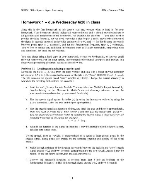
Problem 1.1 – Load<strong>in</strong>g and analyz<strong>in</strong>g a speech signal<br />
Download the file ex1_3.wav from the class website, and save it <strong>in</strong> a folder on your computer<br />
(if you’re <strong>in</strong> SAV 137, the suggested location for the file is C:\Temp\<strong>SPHSC</strong><strong>503</strong>\ex1_3.wav).<br />
The file conta<strong>in</strong>s the spoken word “zero” sampled at 10 kHz. Change the current direc<strong>to</strong>ry <strong>in</strong><br />
<strong>Matlab</strong> <strong>to</strong> the direc<strong>to</strong>ry that conta<strong>in</strong>s the saved file.<br />
a. Load the ex1_3.wav file <strong>in</strong><strong>to</strong> <strong>Matlab</strong>. You can either use <strong>Matlab</strong>’s Import Wizard, by<br />
double-click<strong>in</strong>g on the filename <strong>in</strong> <strong>Matlab</strong>’s current direc<strong>to</strong>ry w<strong>in</strong>dow, or use the<br />
wavread command (see help wavread for details).<br />
b. Plot the speech signal aga<strong>in</strong>st its <strong>in</strong>dex (n) by us<strong>in</strong>g the <strong>in</strong>teractive <strong>to</strong>ols or by us<strong>in</strong>g the<br />
plot command. Label the axes and the plot appropriately.<br />
c. Plot the speech signal as a function of time, and label the axes and the plot appropriately.<br />
H<strong>in</strong>t: you need <strong>to</strong> create the a ‘time’ vec<strong>to</strong>r t, and then plot the signal with “plot(t,y)”.<br />
You can create the correct time vec<strong>to</strong>r by divid<strong>in</strong>g the speech signal’s <strong>in</strong>dex vec<strong>to</strong>r by the<br />
sampl<strong>in</strong>g frequency of the signal, for example:<br />
t = n / fs;<br />
d. What is the duration of the signal <strong>in</strong> seconds? It may be helpful <strong>to</strong> use the figure’s zoom,<br />
pan and data cursor <strong>to</strong>ols.<br />
Voiced speech, such as vowels, is characterized by a series of high-energy peaks <strong>in</strong> the<br />
speech signal. Those peaks are created by the repeated open<strong>in</strong>g and clos<strong>in</strong>g of the vocal<br />
chords.<br />
e. Make a rough estimate of the distance <strong>in</strong> seconds between the peaks <strong>in</strong> the “zero” speech<br />
signal around t=0.2 and t=0.4 seconds, correspond<strong>in</strong>g <strong>to</strong> the two vowels. Aga<strong>in</strong>, it may be<br />
helpful <strong>to</strong> use the figure’s zoom, pan and data cursor <strong>to</strong>ols.<br />
f. Convert the measured distances <strong>in</strong> seconds from part e <strong>in</strong><strong>to</strong> an estimate of the<br />
fundamental frequency (<strong>in</strong> Hz) of the speech signal around t=0.2 and t=0.4 seconds.<br />
– 1 –
<strong>SPHSC</strong> <strong>503</strong> – Speech Signal Process<strong>in</strong>g UW – Summer 2006<br />
Problem 1.2 – Measur<strong>in</strong>g fundamental frequency with correlation<br />
In problem 1.1f, you’ve manually found an estimate for the fundamental frequency of the speech<br />
signal. In this problem, we will use a technique called correlation <strong>to</strong> estimate the fundamental<br />
frequency au<strong>to</strong>matically. Correlation is a measure of the degree <strong>to</strong> which two sequences are<br />
similar. It is related <strong>to</strong> convolution, and its mathematical expression looks like the convolution<br />
sum. There are two k<strong>in</strong>ds of correlation: au<strong>to</strong>-correlation (correlation between a signal and itself)<br />
and cross-correlation (correlation between two different signals). They are def<strong>in</strong>ed as follows:<br />
Au<strong>to</strong>-correlation: r [] l = xnxn [ ][ −l]<br />
xx<br />
∞<br />
∑<br />
n=−∞<br />
Cross-correlation: r [] l = x[ n] y[ n−l]<br />
xy<br />
∞<br />
∑<br />
n=−∞<br />
In <strong>Matlab</strong>, both types of correlation can be computed us<strong>in</strong>g the xcorr function from the Signal<br />
Process<strong>in</strong>g Toolbox. For example,<br />
>> x = [1 1 1]; lmax = 3;<br />
>> [rxx,l] = xcorr(x,lmax);<br />
>> stem(l,rxx); % a triangle<br />
computes and <strong>plots</strong> the au<strong>to</strong>-correlation of x,<br />
r [] xx<br />
l<br />
, for l=-lmax,…,lmax. Similarly,<br />
>> x = [1 1 1]; y = [-1 0 1]; lmax = 3;<br />
>> [rxy,l] = xcorr(x,y,lmax);<br />
>> stem(l,rxy); % 2 up, 2 down<br />
computes and <strong>plots</strong> the cross-correlation of x and y,<br />
r [] xy<br />
l<br />
, for l=-lmax,…,lmax.<br />
a. Clear the workspace (clear), load the speech signal from problem 1.1 aga<strong>in</strong>, and extract<br />
a voiced section of the speech signal us<strong>in</strong>g yvoiced1 = y(1900:2300); . Plot the<br />
voiced section aga<strong>in</strong>st its <strong>in</strong>dex, nvoiced1 = 1900:2300; .<br />
b. Compute and plot the au<strong>to</strong>correlation of the voiced section for lmax=250. You can<br />
modify the example code above <strong>to</strong> do this. Label your x-axis as ‘Lag (<strong>in</strong> samples)’.<br />
Notice the follow<strong>in</strong>g <strong>in</strong> your plot of the au<strong>to</strong>correlation: the au<strong>to</strong>correlation has the highest peak<br />
for zero lag (l=0). This is a necessary property of all au<strong>to</strong>correlations. Then the au<strong>to</strong>correlation<br />
has strong positive peaks at equal distances <strong>to</strong> the left and right of the zero lag po<strong>in</strong>t.<br />
c. Determ<strong>in</strong>e the value of the lag for the next strongest peak <strong>to</strong> the left and right. The zoom<br />
<strong>to</strong>ols of the plot w<strong>in</strong>dow may be helpful for this.<br />
d. Divide the value of the lag you found <strong>in</strong> part e by the sampl<strong>in</strong>g frequency <strong>to</strong> get the value<br />
of the lag <strong>in</strong> seconds.<br />
e. The value of the lag <strong>in</strong> seconds should correspond more or less <strong>to</strong> the distance between<br />
the peaks you found <strong>in</strong> problem 1.1e for t=0.2. Is that the case for you? Convert the value<br />
of the lag <strong>in</strong> seconds <strong>to</strong> a frequency <strong>in</strong> Hz. This value should correspond <strong>to</strong> the<br />
fundamental frequency from problem 1.1f for t=0.2.<br />
f. Repeat a-e for the second voiced section around t=0.4, nvoiced2 = 3800:4200;.<br />
– 2 –
<strong>SPHSC</strong> <strong>503</strong> – Speech Signal Process<strong>in</strong>g UW – Summer 2006<br />
Problem 1.3 – Measur<strong>in</strong>g fundamental frequency with a pitch estima<strong>to</strong>r<br />
It is possible <strong>to</strong> fully au<strong>to</strong>mate the estimation of the fundamental frequency of a speech signal<br />
with the methods used <strong>in</strong> problem 1.1 and 1.2. In this problem, we will use a pitch estima<strong>to</strong>r <strong>to</strong><br />
estimate the pitch of the entire speech signal.<br />
a. Download the file pitchestimate.m from the class website. This m-file conta<strong>in</strong>s the<br />
<strong>Matlab</strong> function pitchestimate, which can be used as follows<br />
% y,fs is the <strong>in</strong>put signal and sampl<strong>in</strong>g frequency<br />
>> [t,p]=pitchestimate(y,fs);<br />
% t is the times at which the fundamental frequency was estimated<br />
% p is the estimates of the fundamental frequency<br />
>> plot(t,p)<br />
See help pitchestimate for details.<br />
b. Clear the workspace, load the speech signal aga<strong>in</strong>, and estimate and plot its fundamental<br />
frequency us<strong>in</strong>g the pitchestimate function.<br />
c. [optional] If you have access <strong>to</strong> a microphone, it could be <strong>in</strong>terest<strong>in</strong>g <strong>to</strong> record your own<br />
voice and determ<strong>in</strong>e your own fundamental frequency.<br />
– 3 –