8 TECHNIQUES OF INTEGRATION

8 TECHNIQUES OF INTEGRATION
8.1 INTEGRATION BY PARTS
SUGGESTED TIME AND EMPHASIS
1 1 2
classes Essential material
POINTS TO STRESS
1. The method of integration by parts; how to choose u and dv to make the resulting integral simpler.
2. The analogy with u-substitution: u-substitution is “undoing” the Chain Rule, and integration by parts is
“undoing” the Product Rule.
QUIZ QUESTIONS
• Text Question: Example 1 is an attempt to integrate x sin x. As stated in the subsequent note, it is
possible, using integration by parts, to obtain ∫ x sin xdx = 1 2 x2 sin x − 1 ∫
2 x 2 cos xdx. Why is this
equation an indication that we didn’t choose our u and dv wisely?
Answer: We are trying to integrate x sin x. Ifwehavetointegratex 2 cos x we have made the problem
more complicated, not less complicated.
• Drill Question: Compute ∫ √ t ln tdt.
Answer: 4 (√ ) 3 √
3 t ln t −
4
(√ ) 3
9
t + C
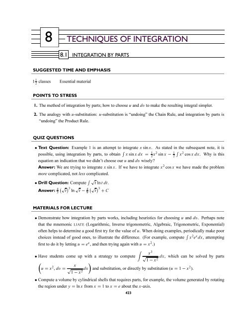
MATERIALS FOR LECTURE
• Demonstrate how integration by parts works, including heuristics for choosing u and dv. Perhaps note
that the mnemonic LIATE (Logarithmic, Inverse trigonometric, Algebraic, Trigonometric, Exponential)
often helps to determine a good first try for the value of u. When doing examples, periodically make poor
choices instead of good ones, to illustrate the difference. (For example, compute ∫ x 2 e x dx, attempting
first to do it by letting u = e x , and then trying again with u = x 2 .)
∫
x 3
• Have students come up with a strategy to compute √ dx, which can be solved by parts
1 − x 2
(
)
u = x 2 x
, dv = √ dx and substitution, or directly by substitution (u = 1 − x 2 ).
1 − x 2
• Compute a volume by cylindrical shells that requires parts, for example, the volume generated by rotating
the region under y = ln x from x = 1tox = e about the x-axis.
423

CHAPTER 8
TECHNIQUES OF INTEGRATION
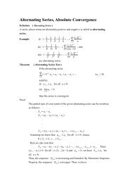
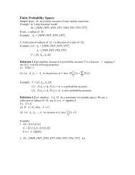
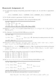
• Draw a function like the one below and have the students try to approximate ∫ 2
0 xg′′ (x) dx.
y
3
2
1
0
1 2 3 x
Answer: ∫ 2
0 xg′′ (x) dx ≈ 2g ′ (2) − g (2) − 0g ′ (0) + g (0) ≈ 2 (1) − 2 + 0.4 = 0.4
WORKSHOP/DISCUSSION
• Compute a definite integral that requires integration by parts (such as ∫ π/2
0
x sin xdx).
• Solve a problem that requires first a substitution, then integration by parts, such as
∫ ( 2xe x2) (
sin
ln e x2) dx.
Answer: ∫ ( 2xe x2) sin
(
ln e x2) dx = 1 2 ex2 sin ln e x2 − cos ln e x2 + C
• Work through a non-trivial integration by parts problem with the students, such as ∫ x 3 ln ( 2 + x 2) dx.
Note that it can be solved in two steps, using the substitution u = 2 + x 2 and then using parts on
∫
(u − 2) ln udu.
1
2
GROUP WORK 1: Guess the Method
Divide the students into groups and put problems on the board from the list of examples below (or hand out
the problems, if you prefer). Either have the students integrate the expressions completely, or describe what
method they would use, and what their answer should look like. For closure, do a few problems as a class that
were not covered in the group work.
Examples:
∫ x ln 3xdx=
1
2
x 2 ln 3x − 1 4 x2 + C
∫ e 2x sin e x dx = sin e x − e x cos e x + C
(substitution, then parts)
∫ e 2x cos xdx= 1 5 e2x sin x + 2 5 e2x cos x + C
(parts twice with a subtraction)
∫ x 3 cos x 2 dx = 1 2 x2 sin ( x 2) + 1 2 cos ( x 2) + C
(substitution, then parts)
∫ ( x 2 + x
2 ) ln ( 2 + x 2) dx = 1 (
4 2 + x
2 ) ln ( 2 + x 2) − 1 (
8 2 + x
2 ) 2 + C (substitution, then parts)
∫ x 2 (ln x) 2 dx = 1 3 x3 (ln x) 2 − 2 9 x3 ln x + 2 27 x3 + C
∫
cos
√ xdx= cos
(√ x
) +
√ x sin
√ x + C
424
(parts twice)
(substitution, then parts)

SECTION 8.1
INTEGRATION BY PARTS
GROUP WORK 2: Find the Error
Notice that the answers to the two problems are completely different. Give them the first problem, only
revealing the existence of the second after they’ve solved the first.
Answers:
1. The stranger forgot the constant of integration. The last line should read 0 =−1 + C, which is true.
One cute hint you can give the students (if you dare) is as follows:
‘There is something that the stranger failed to “C”. All you have to do is “C” it and you will have the
solution to the problem. Do you “C” what I mean?’
2. The penultimate line should read ∫ π/4
π/6
tan xdx =−1|π/4
π/6 + ∫ π/4
π/6
tan xdx, which gives 0 = 0—atrue
statement.
HOMEWORK PROBLEMS
Core Exercises: 1, 15, 20, 23, 34, 46, 55, 62
Sample Assignment: 1, 6, 9, 15, 20, 23, 29, 34, 38, 40, 43, 46, 47, 55, 58, 62, 67
Exercise D A N G
1 ×
6 ×
9 ×
15 ×
20 ×
23 ×
29 ×
34 ×
38 ×
40 × ×
43 ×
46 ×
47 ×
55 × ×
58 ×
62 × ×
67 × ×
425

GROUP WORK 1, SECTION 8.1
Guess the Method
What method(s) could be used to compute the following antiderivatives? Either compute them explicitly, or
describe the best method to use.
1. ∫ x ln 3xdx
2. ∫ e 2x sin e x dx
3. ∫ e 2x cos xdx
4. ∫ x 3 cos x 2 dx
5. ∫ x ( 2 + x 2) ln ( 2 + x 2) dx
6. ∫ x 2 (ln x) 2 dx
7. ∫ cos √ xdx
426

GROUP WORK 2, SECTION 8.1
Find the Error
It is a beautiful Spring day. You leave your calculus class feeling sad and depressed. You aren’t sad because of
the class itself. On the contrary, you have just learned an amazing integration technique: Integration by Parts.
You aren’t sad because it is your birthday. On the contrary, you are still young enough to actually be happy
about it. You are sad because you know that every time you learn something really wonderful in calculus,
a wild-eyed stranger runs up to you and shows you a “proof” that it is false. Sure enough, as you cross the
street, he is waiting on the other side.
“Good morning, Kiddo,” he says.
“I just learned integration by parts. Let me have it.”
“What do you mean?” he asks.
“Aren’t you going to run around telling me that all of math is lies?”
“Well, if you insist,” he chuckles... and hands you a piece of paper:
“Hey,” you say, “I don’t get it! You did everything right this time!”
“Yup!” says the hungry looking stranger.
“But... Zero isn’t equal to negative one!”
“Nope!” he says.
You didn’t think he could pique your interest again, but he has. Spite him. Find the error in his reasoning.
427

GROUP WORK 2, SECTION 8.1
Find the Error (The Sequel)
What a wonderful day! You have survived another encounter with the wild-eyed stranger, demolishing his
mischievous pseudo-proof. As you leave his side, you can’t resist a taunt.
“Didn’t your mother tell you never to forget your constants?” It seemed a better taunt when you were thinking
it than it did when you said it.
“Eh?” he says. You come up to him again.
“I was just teasing you. Just pointing out that when doing indefinite integration, those constants should not be
forgotten. A simple, silly error, not worthy of you.” You look smug. You are the victor.
“Yup. Indefinite integrals always have those pesky constants.” For some reason he isn’t looking defeated. He
is looking crafty.
“Right. Well, I’m going to be going now...”
“Of course, Kiddo, definite integrals don’t have constants, sure as elephants don’t have exoskeletons.”
“Yes. Well, I really must be going.”
Surprisingly quickly, he snatches the paper out of your hand, and adds to it. This is what it now looks like.
“No constants missing here! Happy Birthday!” The stranger leaves, singing the “Happy Birthday” song in a
minor key. Now there are no constants involved in the argument. But the conclusion is the same: 0 =−1. Is
the stranger right? Has he finally demonstrated that all that you’ve learned is suspect and contradictory? Or
can you, using your best mathematical might, find the error in this new version of his argument?
428

8.2 TRIGONOMETRIC INTEGRALS
SUGGESTED TIME AND EMPHASIS
1 class Recommended material
POINTS TO STRESS
1. Integration of powers of the sine and cosine functions.
2. Integration of powers of the tangent and secant functions.
QUIZ QUESTIONS
• Text Question: When m is odd, we can integrate ∫ sin m xdxby letting u = cos x. Whydoesm have to
be odd for this trick to work?
Answer: When m is odd, we can write sin m xdx as ( 1 − cos 2 x ) (m−1)/2 sin xdx, and then the
u-substitution works. If m is not odd, then (m − 1) /2 is not an integer. Less formal answers that correctly
address the issue of parity should be given credit.
• Drill Question: Compute ∫ sin 2 x cos 3 xdx.
Answer: − 1 5 sin5 x + 1 3 sin3 x + C
MATERIALS FOR LECTURE
∫
• Give several examples, such as sin 4 x cos 3 ∫
xdx, sin 7 x 3√ cos xdx,
∫ sin x (cos x) −1 dx to review the strategies for evaluating ∫ sin m x cos n xdx:
∫ sin 2 x cos 4 xdx,
and
• If m or n isodd,peeloffonepowerofsinx or cos x and use sin 2 x + cos 2 x = 1.
• If m and n are both even, use the half-angle identities, as done in the text.
Answers:
∫ sin 4 x cos 3 xdx= ∫ sin 4 x ( 1 − sin 2 x ) cos xdx. Letting u = sin x gives
∫
u
4 ( 1 − u 2) du = 1 5 sin5 x − 1 7 sin7 x + C
∫ sin 7 x 3√ cos xdx= ∫( 1 − cos 2 x ) 3 cos 1/3 x sin xdx. Letting u = cos x gives
∫ ( 1 − u 2) 3
u 1/3 du =−22 3 (cos x)22/3 +
16 9 (cos x)16/3 −
10 9 (cos x)10/3 + 3 4 (cos x)4/3 + C
∫ ( )
∫ 1 − cos 2x 2 ( ) 1 + cos 2x 4
sin 2 x cos 4 xdx=
dx
2
2
=
64
1 ∫( 1 + 2cos2x − cos 2 2x − 4cos 3 2x − cos 4 2x + 2cos 5 2x + cos 6 2x ) dx
The odd powers of cos 2x can now be integrated by the previous method. The even powers require further
use of the half-angle identities.
∫ sin x (cos x) −1 dx = ∫ tan xdx= ln |sec x| + C
• Give a couple of examples such as ∫ √ tan x sec 4 xdx and ∫ tan x sec 3.28 xdx to illustrate the
straightforward cases of ∫ tan m x sec n xdx.
429

CHAPTER 8
TECHNIQUES OF INTEGRATION
∫ √
Answers: tan x sec 4 xdx = ∫ [√ tan x ( tan 2 x + 1 )] sec 2 xdx. Letting u = tan x gives
∫
u
1/2 ( u 2 + 1 ) du = 2 3 (tan x)3/2 + 2 7 tan x7/2 + C.
∫ tan x sec 3.28 xdx= ∫ sec 2.28 (tan x sec x) dx. Letting u = sec x gives ∫ u 2.28 du = sec3.28 x
+ C.
3.28
• Derive the equation ∫ π
−π sin mx cos nx dx = 0intwoways,firstbycomputing∫ sin mx cos mx dx using
Formula 2 and then by simply noting that sin mx cos nx is an odd function.
WORKSHOP/DISCUSSION
• Derive the equation ∫ sec xdx= ln |sec x + tan x| + C. Use this equation to compute ∫ tan 4 x sec xdx.
• Show how the computation of ∫ tan 5 xdxis quite different from the previous computation.
• Use the double-angle formula cos 2 1 + cos 2θ
θ = to compute ∫ dθ
2
1 + cos 2θ .
• Have the students find the volume generated by rotating the region under y = 1 + sin 2 x,0≤ x ≤ π about
the x-axis.
GROUP WORK 1: An Equality Tester
This activity thoroughly explores a family of integrals that are interesting in their own right, using a computation
that comes in handy in the study of Fourier series.
It is best to pose Problem 1 before handing out the sheet, because the students may disagree on the relative
areas of the two functions before they see Problem 2.
For Problem 2, the students may need the hint to consider the cases m = n and m ≠ n separately.
Answers:
1. (a)
y
1
0 ¹ 2¹
One has thrice the period of the other. ∫ 2π
0
sin 2 3xdx= ∫ 2π
0
sin 2 xdx= π
(b) ∫ 2π
0
sin 2 mx dx = π if m is an integer not equal to zero; ∫ 2π
0
sin 2 mx dx = 0ifm = 0.
2. (a) ∫ 2π
0
sin mx sin nx dx = 0ifm and n are positive integers with m ≠ n. (This can be proven by
computation, and illustrated by graphical analysis.)
∫ 2π
0
sin mx sin nx dx = π if m and n are positive nonzero integers with m = n, by Problem 1(b).
(b) Again, this can be seen by direct computation, or using the hint and the fact that
cos mx cos nx − sin mx sin nx = cos (m + n) x
(c) ∫ 2π
0
cos mx cos nx dx = 0ifm and n are positive integers with m ≠ n; ∫ 2π
0
cos mx cos nx dx = π if
m and n are positive nonzero integers with m = n.
430
x

SECTION 8.2
TRIGONOMETRIC INTEGRALS
GROUP WORK 2: Find the Error
Introduce this activity by writing
A = B
C = D
on the blackboard and asking, “If A = C, can we conclude that B = D?” Then hand out the exercise. If
students answer the problem by simply saying, “He forgot the + C,” make sure that they understand the
implication of the stranger’s computations, namely, that the functions y = cos 2x and y = 2cos 2 x differ by
a constant.
HOMEWORK PROBLEMS
Core Exercises: 3, 8, 13, 31, 52, 55, 57, 62
Sample Assignment: 3, 8, 13, 26, 31, 46, 47, 52, 55, 57, 59, 62, 66, 67
Exercise D A N G
3 ×
8 ×
13 ×
26 ×
31 ×
46 ×
47 ×
52 × ×
55 ×
57 ×
59 ×
62 ×
66 × ×
67 ×
431

GROUP WORK 1, SECTION 8.2
An Equality Tester
1. (a) Graph sin 2 x and sin 2 3x for 0 ≤ x ≤ 2π. What is the relationship between these two functions?
What do you think is the relationship between the areas bounded by these two functions from 0 to
2π?
(b) Let m ≥ 0 be an integer. Compute ∫ 2π
0
sin 2 mx dx.
2. Let m and n be nonnegative integers.
(a) Compute ∫ 2π
0
sin mx sin nx dx.
(b) Show that ∫ 2π
0
sin mx sin nx dx = ∫ 2π
0
cos mx cos nx dx.
Hint: Consider ∫ 2π
0
(cos mx cos nx − sin mx sin nx) dx.
(c) Compute ∫ 2π
0
cos mx cos nx dx.
432

GROUP WORK 2, SECTION 8.2
Find the Error
It is a beautiful Spring morning. Everywhere you look, people are happily going to their classes, or coming
from their classes. “High School is fun!” calls out one student, and about twenty more yell “Sure is!”
in unison. Someone else calls out, “I love History!” A bunch of other students call “Great subject!” in
response. Swept up in the spirit of things, you call out, “Calculus is wonderful!” “Lies! Lies!” calls out a
lone, familiar voice. You wheel around and directly behind you is a wild-eyed hungry-looking stranger.
“Oh, don’t be silly,” you say. “I just learned about trigonometric integration. It wasn’t that hard a section, and
thereisn’tasinglelieinit.”
He looks up at you and says, “Oh, really? Perhaps you can take a quick true/false quiz, and see how easy the
section is.” The stranger then whips out a sheet of paper with this on it:
“Both are clearly true!” he shouts, before you have a chance to think. “AND we know that
−2sin2x =−2 (2sinx cos x) =−4sinx cos x! Thus cos 2x = 2cos 2 x! Hoho!”
“Ho ho?” you ask.
“‘Ho ho,’ I say; ho, ho, I mean! Because at x = 0, cos 2x = 1, and 2 cos 2 x = 2! Once again, your
‘Calculus’ gets you into trouble! ‘Two equals one, two equals one!”’ sings the stranger, to the tune of “Nyah,
nyah, nyah nyah, nyah,” as he skips off into the distance.
Consider the stranger’s test. Are the answers “true” to both questions? And if so, then could the stranger
be correct? If 1 = 2, then how can you tell odd numbers from even ones? Would one still be the loneliest
number? How many turtle doves would your true love give to you on the second day of Christmas? Or is
there a possibility that there is an error somewhere in the stranger’s reasoning? Find the error.
433

8.3 TRIGONOMETRIC SUBSTITUTION
SUGGESTED TIME AND EMPHASIS
1
2
– 1 class Recommended material
POINTS TO STRESS
1. The basic trigonometric substitutions and when to use them.
2. The use of trigonometric identities and right-triangle trigonometry to convert antiderivatives back to
∫
dx
expressions in the original variable, for example, ( 1 + x 2 ) 3/2 = sin ( tan −1 x ) x
= √ .
1 + x 2
QUIZ QUESTIONS
• Text Question: The book states that when doing an integral where the term 1 + x 2 occurs, it often helps
to use the substitution x = tan θ. How could introducing a trigonometric function possibly make things
simpler?
Answer: This substitution allows us to use the simplifying identity 1 + tan 2 θ = sec 2 θ.
• Drill Question: Compute ∫ 1
0
√
4 − x 2 dx using the substitution x = 2sint and the fact that
∫ cos 2 tdt= 1 2 cos t sin t + 1 2 t + C
Answer: 1 2√
3 +
1
3
π
MATERIALS FOR LECTURE
• Go over the table of trigonometric substitutions listed below, emphasizing when to use the different forms,
and the restrictions that need to be placed on θ for each.
∫
Examples:
Expression Substitution Identity
√
a 2 − x 2 x = a sin θ, − π 2 ≤ θ ≤ π 2
1 − sin 2 θ = cos 2 θ
a 2 + x 2 x = a tan θ, − π 2 ≤ θ ≤ π 2
1 + tan 2 θ = sec 2 θ
√
x 2 − a 2 x = a sec θ,0≤ θ ≤ π 2 or π ≤ θ ≤ 3π 2
sec 2 θ − 1 = tan 2 θ
∫
dx
√ = arcsin 1 25 − x 2 5 x + C,
dx
1 + 9x 2 = 1 3
arctan 3x + C
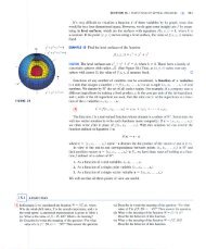
• Show how to derive identities such as sin ( tan −1 x ) x
= √ by setting up a right triangle as in Figure 1.
x 2 + 1
• Have the students evaluate ∫ √ 1 − x − x 2 dx in two ways: first by completing the square, and then using
the trigonometric substitution x + 1 √
2 = 5
2
sin θ.
434

SECTION 8.3
TRIGONOMETRIC SUBSTITUTION
WORKSHOP/DISCUSSION
• Compute ∫ 1
0 x2√ 4 − x 2 dx using a trigonometric substitution. Point out that because this is a definite
integral, we don’t need to use trigonometric identities at the end to find the antiderivative in terms of the
original variable x.
∫ 1
Answer:
0 x2√ 4 − x 2 dx = 16 ∫ π/6
0
sin 2 u cos 2 udu using the substitution 2 sin u = x, and
16 ∫ π/6
0
sin 2 u cos 2 udu=− 1 4√
3 +
1
3
π.
• Evaluate ∫ x 2√ x 2 − a 2 dx in two different ways and compare the computations: first use the trigonometric
substitution x = a sec θ, then use the hyperbolic substitution x = a cosh t.
GROUP WORK 1: Pizza for Three
The introduction to this exercise is very important. The goal is to slice a
14 ′′ pizza, with two parallel lines across the entire pizza, to create three
pieces of equal area.
Draw the figure on the board and explain that they need to find the value of
c. (If the class is particularly quick, the introduction can be abbreviated, but
it is better to say too much here than too little.)
This problem is also a good excuse to order pizza for a hard-working class.
Note that this is Problem 1 from Problems Plus after Chapter 8. A complete
solution to this problem can be found in the Solutions Manual.
Answer: c ≈ 1.855
y
7
_7 _c c 7
_7
x
GROUP WORK 2: Look Before You Compute
The goal of this activity is to show students that it sometimes pays to look at the geometry of a problem before
immediately applying techniques.
Answers:
1. √ 12 + 4x − x 2 = √ 4 2 − (x − 2) 2
2. 4sinθ = x − 2gives ∫ π/2
−π/2 16 cos2 θ dθ = 8π.
3.
y
4
2
_2 0 2 4 6 x
This is a semicircle of radius 4 and center (0, 2) with equation (x − 2) 2 + y 2 = 16.
435

CHAPTER 8
TECHNIQUES OF INTEGRATION
HOMEWORK PROBLEMS
Core Exercises: 1, 12, 22, 32, 36, 40
Sample Assignment: 1, 4, 12, 19, 22, 25, 32, 33, 34, 36, 37, 39, 40, 42
Exercise D A N G
1 × ×
4 ×
12 ×
19 ×
22 ×
25 ×
32 ×
33 ×
34 ×
36 × ×
37 ×
39 × ×
40 ×
42 ×
436

GROUP WORK 1, SECTION 8.3
Pizza for Three
How do you cut a 14 ′′ pizza into three pieces of equal area, using just two parallel cuts?
y
7
_7 _c c 7
x
_7
437

GROUP WORK 2, SECTION 8.3
Look Before You Compute
Consider the definite integral
∫ 6
−2
√
12 + 4x − x 2 dx
1. Rewrite the integrand in the form √ b 2 − (x − a) 2 .
2. Use a trigonometric substitution to evaluate the integral.
3. Graph the original integrand over the range [−2, 6]. Evaluate the integral directly by interpreting it as an
area.
438

8.4 INTEGRATION OF RATIONAL FUNCTIONS BY PARTIAL FRACTIONS
SUGGESTED TIME AND EMPHASIS
1
2 –11 2
classes Optional material
POINT TO STRESS
The idea that a given rational function can be broken down into a set of standard integrals, each of which
can be computed routinely.
QUIZ QUESTIONS
1
• Text Question: Why would one want to write
as the sum of two fractions?
(x + 2)(x + 3)
∫ ∫
∫
dx
Answer: It is much easier to find
x + 2 and dx
x + 3 than it is to find dx
(x + 2)(x + 3) directly.
∫
dx
• Drill Question: Compute
x 2 − 3x + 2 .
Answer: ln |x − 1| + ln |x − 2| + C
MATERIALS FOR LECTURE
∫
• As a warm-up, remind students how to compute
∫
becoveredindepth,alsocompute
∫
dx
x 2 + 4x + 8 =
∫
A
x + a dx and
dx
(x + 2) 2 + 4 .
B
dx. If partial fractions are to
2
(x + a)
• Remind students of the process of polynomial division, perhaps by rewriting 2x3 + 3x 2 + 7x + 4
2x + 1
x 2 + x + 3 + 1
∫ 2x 3
2x + 1 , and then computing + 3x 2 + 7x + 4
dx.
2x + 1
• Be sure to indicate that in order to use partial fractions, we need the degree of the numerator less than
∫ x 4 + 2
the degree of the denominator. So to compute
x 2 dx, we first use long division to rewrite it as
− 1
∫ (
x 2 + 1 + 3
x 2 − 1
)
dx.
∫
x + 3
• Find the coefficients for the partial fraction decomposition for
dx in two different ways:
(x − 2)(x − 1)
first using two linear equations, and then using the method of creating zeros [setting x = 1andthen
x =−2inx + 3 = A (x + 2) + B (x − 1)].
3
• Go over the process of partial fractions for quadratic terms, using ( x 2 + 2 ) (x − 1) = 1
x − 1 − x + 1
x 2 + 2 ,
1
and (if the subject is to be covered exhaustively) ( x 2 + 1 ) = 1 2 x x − x
x 2 + 1 − x
( x 2 + 1 ) 2 .
as
439

CHAPTER 8
TECHNIQUES OF INTEGRATION
WORKSHOP/DISCUSSION
• Go over the process of partial fractions for products of powers of linear terms, starting with
x − 7
(x − 2)(x + 3) = −1
x − 2 + 2
x + 3 , and continuing with 3x2 − x − 3
(x + 1) x 2 = 1
x + 1 + 2 x − 3 x 2 .
1
• Point out that the quadratic in the denominator of f (x) =
x 2 is not irreducible. It can be factored
+ x − 6
into the two linear terms x − 2andx + 3, and so the partial fraction decomposition is found by writing
1
x 2 + x − 6 = A
x + 2 + B and solving for A and B.
x − 3
• Show the students how a complicated partial fractions problem would be set up, without trying to solve it.
∫
5x + 3
An example is
x 3 (x + 1) ( x 2 + x + 4 )( x 2 + 3 ) 2 dx.
∫
2x − 1
• Work through examples such as
x 2 dx where the method of partial fractions should be avoided.
− x − 2
GROUP WORK 1: Partial Fractions
Two versions of this group activity are provided. The instructor should select the appropriate version for the
depth at which this topic is to be covered.
Answers:
Version 1
1. (a) ln |x − 1| + C (b) ln |x + 3| + C 2. (x + 3)(x − 1)
∫
xdx
3.
(x + 3)(x − 1) = 3 4 ln (x + 3) + 1 4
ln (x − 1) + C
∫
(5x + 5) dx
4.
(x + 3)(x − 1) = 5 2 ln (x + 3) + 5 2
ln (x − 1) + C
Version 2
1. (a) ln |x + 1| + C (b) ln |x + 2| + C 2. 2x (x + 2)(x + 1)
3. 3 4 ln |x| − 1 4 ln |x + 2| − 1 2
ln |x + 1| + C
4. 1 2 ln |x| + 1 2 ln |x + 2| + 1 2
ln |x + 1| + C
Version 3
( )
1. (a) ln |x + 1| + C (b) ln |x + 2| + C (c) 1 2 tan−1 1
2
x + C 2. (x + 2)(x + 1) ( x 2 + 4 )
3. −10 ln (x + 2) + 4ln(x + 1) + 3ln ( x 2 + 4 ) + 2 arctan 1 2 x + C
4. x − 10 ln (x + 2) + 4ln(x + 1) + 3ln ( x 2 + 4 ) + 2 arctan 1 2 x + C
440

SECTION 8.4
INTEGRATION OF RATIONAL FUNCTIONS BY PARTIAL FRACTIONS
GROUP WORK 2: Finding Coefficients
Answers:
1
1. (a) −
5 (x + 2) + 1
180 (x − 3) + 1
6 (x + 3) 2 + 7
36 (x + 3)
1
2. −
5 (x + 2) + 1
180 (x − 3) + 1
6 (x + 3) 2 + 7
36 (x + 3)
3.
(b) 3 56
3
56
−1 + 5x
x 2 + x + 2 − 3 −26 + 5x
56 x 2 − 4x − 4
−1 + 5x
x 2 + x + 2 − 3
56
−26 + 5x
x 2 − 4x − 4
HOMEWORK PROBLEMS
Core Exercises: 2, 7, 23, 35, 44, 51, 54, 55, 62
Sample Assignment: 2, 5, 7, 12, 16, 23, 34, 35, 41, 44, 48, 51, 54, 55, 57, 62, 64, 65
Exercise D A N G
2 ×
5 ×
7 ×
12 ×
16 ×
23 ×
34 ×
35 ×
41 ×
44 ×
48 ×
51 ×
54 ×
55 ×
57 × ×
62 ×
64 ×
65 × ×
441

1. Compute the following integrals:
∫
dx
(a)
x − 1
GROUP WORK 1, SECTION 8.4
Partial Fractions (Version 1)
(b)
∫
dx
x + 3
2. Factor x 2 + 2x − 3.
∫
3. Compute
xdx
x 2 + 2x − 3 .
∫
4. Compute
5x + 5
x 2 + 2x − 3 dx. 442

1. Compute the following integrals:
∫
dx
(a)
x + 1
GROUP WORK 1, SECTION 8.4
Partial Fractions (Version 2)
(b)
∫
dx
x + 2
2. Factor 2x 3 + 6x 2 + 4x.
∫
3. Compute
2x + 3
2x 3 + 6x 2 + 4x dx.
∫
4. Compute
3x 2 + 6x + 2
2x 3 + 6x 2 + 4x dx. 443

1. Compute the following integrals:
∫
dx
(a)
x + 1
GROUP WORK 1, SECTION 8.4
Partial Fractions (Version 3)
(b)
∫
dx
x + 2
(c)
∫
dx
x 2 + 4
2. Factor x 4 + 3x 3 + 6x 2 + 12x + 8.
∫
3. Compute
20x 2 dx
x 4 + 3x 3 + 6x 2 + 12x + 8 .
∫ x 4 + 3x 3 + 26x 2 + 12x + 8
4. Compute
x 4 + 3x 3 + 6x 2 + 12x + 8 dx. 444

GROUP WORK 2, SECTION 8.4
Finding Coefficients
1. Write the following rational functions as a product of powers of linear terms and irreducible quadratic
terms.
1
(a) ( x 2 − x − 6 )( x 2 + 6x + 9 )
(b)
3
( x 2 + x − 2 )( x 2 − 4x − 4 )
2. Find the partial fraction decomposition for the function in Problem 1(a) using a linear system.
3. Find the partial fraction decomposition for the function in Problem 1(b) using the method of creating
zeros.
445

8.5 STRATEGY FOR INTEGRATION
SUGGESTED TIME AND EMPHASIS
1 class Optional material
POINTS TO STRESS
1. The four-step strategy suggested in the text.
2. If at first you don’t succeed, try again with a different method.
3. There are elementary functions that do not have elementary antiderivatives
MATERIALS FOR LECTURE
• This section gives the instructor a good opportunity to work a variety of examples with the students. The
following challenging integrals provide opportunities to use the various techniques and strategies:
∫ x
3 √ 1 − x 2 ∫
dx e
x 1/3 ∫
dx
(x ln x) 2 ∫
dx tan −1 ∫ √
xdx cos xdx
∫ ∫
∫ [ ] cos x sin xdx
3dx
ln (ln x) 2 ∫
1 + sin 4 x x 1/2 ( 1
x 3/2 − x 1/2) √ dx x
e − e x dx ∫ x 5 cos x 3 dx
Answers:
∫ x
3 √ ( )
1 − x 2 dx =− 15 (1
x 2 +
15
2 − x
2 ) 3/2 ∫ + C, e
x 1/3 (
dx = 3e x1/3 x 2/3 − 2x 1/3 + 2 ) + C,
∫
(x ln x) 2 dx =
27 1 ( x3 9ln 2 x − 6lnx + 2 ) + C, ∫ tan −1 xdx= x arctan x − 1 2 ln ( x 2 + 1 ) + C,
∫
∫ √ √ √ √ cos x sin x
cos xdx= 2cos x + 2 x sin x + C,
1 + sin 4 x dx = 1 2 arctan ( sin 2 x ) + C,
∫
∫ [ ]
3 dx
ln (ln x) 2
x 2 − x =−3lnx + 3ln(x − 1) + C, √ dx = [ ln 2 (ln x) − 2ln(ln x) + 2 ] ln x + C,
x
∫
dx
e − e x = 1 [ x − ln (e x − e) ] + C, ∫ x 5 cos x 3 dx = 1
e
3 cos x3 + 1 3 x3 sin x 3 + C
∫
dx
• Discuss integrating functions with parameters. For example, compute the antiderivative
x 2 + A by
breaking it into cases. Also examine parameters as part of the limits of integration, as in solving the
∫ a
xdx
equation
3 x 2 − 8 = 2.
• Go through a few integrals that require special approaches, such as ∫ sec xdx.
∫
∫ (sec x + tan x) sec x
Answer: sec xdx=
dx = ln (sec x + tan x) + C
sec x + tan x
WORKSHOP/DISCUSSION
1
• Find the area under the curve f (x) =
e x from x = 1tox = 2. (See Exercise 74.)
+ e−x ∫ 2
dx
Answer:
e x + e −x = arctan e2 − arctan e ≈ 0.218
1
• If the velocity of a particle is given by v (t) =
√ t ln t , determine the distance the particle has traveled
t 2 − 1
from t = 2tot = 5. (See Exercise 56.)
446

SECTION 8.5
STRATEGY FOR INTEGRATION
x
Answer: We let u = ln x, dv = √ , followed by a trigonometric substitution to obtain
∫
x 2 − 1
t ln t
√
t 2 − 1 dt = √ t 2 − 1lnt − √ t 2 − 1 − arcsec t + C. Our final answer is thus
2 √ 6ln5− 2 √ 6 + arcsec 5 − √ 3ln2+ √ 3 − 1 3 π ≈ 3.839.
• If the rate of change of population growth with respect to time is given by b (t) = t3 + 1
t 3 , find the total
− t2 change from year 1 to year 3. (See Exercise 66.)
GROUP WORK 1: Putting It All Together
The students may not understand the idea of taking one step, and describing a strategy. Perhaps do Problem 1
(or a similar problem) for them as an example. In Problem 3, students need to realize that ln x π = π ln x.
Answers:
1. (a) Substitute u = cos x. (b) ∫ e 5cosx sin x cos 2 xdx=− ∫ u 2 e 5u du
(c) Integrate by parts (twice).
2. (a) Substitute x = u 3 . (b) ∫ dx
x 2/3 + 3x 1/3 + 2 = 3 ∫
(c) Use long division and then partial fractions.
u 2 du
u 2 + 3u + 2
3. (a) Note that ln (x π ) = π ln x. (b) ∫ x 5 ln (x π ) dx = ∫ πx 5 ln xdx
(c) Integrate by parts with u = ln x.
4. (a) Integrate by parts with u = ln (1 + e x ), dv = e 2x dx.
∫
(b) e 2x ln (1 + e x ) dx = 1 2 e2x ln (1 + e x ) − 1 ∫
e 2x
2 1 + e x ex dx
(c) Substitute u = 1 + e x or u = e x .
5. (a) Expand (e x + cos x) 2 = e 2x + 2e x cos x + cos 2 x.
(b) ∫ (e x + cos x) 2 dx = ∫ e 2x dx + 2 ∫ e x cos xdx+ ∫ cos 2 xdx
(c) The first and third integrals are simple, and the second can be integrated by parts (twice).
∫ ln (ln x)
6. (a) Substitute u = ln x. (b) dx = ∫ ln udu (c) Integrate by parts.
x
GROUP WORK 2: Integration Jeopardy
This activity, designed to last for sixty to ninety minutes, is meant as a computational review of integration
techniques. Technology should not be permitted.
The Integration Jeopardy game board should be put on an overhead projector, or copied onto the blackboard.
The game is played in two rounds, each consisting of 20 questions, followed by a third round with a final
question. Students should be put into at most six mixed-ability teams of between three and seven players per
team. (It is most fun for the students if they get to name their team, but this process can take time!)
447

CHAPTER 8
TECHNIQUES OF INTEGRATION
Round 1: Jeopardy
Each square on the game board corresponds to a question. The next question is chosen by the player who
answered the previous question correctly. (The first question is chosen by a randomly selected student.) Each
team sends a representative up to the blackboard. The teacher reads the question aloud, or writes it on the
blackboard. The representatives all work, simultaneously, trying to figure out the correct answer. The students
who are not at the blackboard also work on the problems.
The first person at the board who is confident in his or her answer slaps the board (or rings a bell, or blows
a whistle) to alert the teacher. All of the other students put down their pencils and their chalk. The student
who slapped the board first then announces the answer in a loud, clear voice. Every team in turn gets a chance
to challenge the given answer. (So the students who are not at the board have a real incentive to work on
the problem, because they may have an opportunity to challenge.) A correct answer or challenge earns the
designated value for the team. An incorrect answer or challenge causes half of that value to be deducted from
the team’s total. A team can have negative as well as positive money. (If nobody challenges an incorrect
answer, no money is awarded or deducted, and the teacher corrects the answer.)
After each question is asked, it should be crossed off the game board. Round 1 ends when the class is half
over, regardless of whether all the questions have been asked and answered. If this is run as a sixty-minute
activity, only about half of the questions will be asked.
Round 2: Double Jeopardy
This works the same as Round 1, except all the dollar values are doubled. Round 2 ends when there are only
eight minutes of class left.
Round 3: Final Jeopardy
Each team gets to wager an amount anywhere from $300 up to their total. (They can always wager at least
$300.) Each team writes their name and wager on a slip of paper, and these wagers are collected by the
teacher. Then the Final Jeopardy question is asked. The teams have four minutes to come up with a consensus
answer. After these are all written down and handed in, the solution is revealed by the teacher, and then each
team’s answer and wager are announced. Correct answers win the amount wagered, while incorrect answers
lose that amount. The winning team is applauded, and the activity is done.
Optional Rule: The Daily Double
One question from each of the first two rounds can be secretly designated by the teacher as a “Daily Double.”
When a team picks the “Daily Double,” they have to answer the question by themselves, in two minutes or
less. The value is chosen by them, from $100 to their total worth. (They can always wager at least $100.)
After they have given their answer, every other team is free to challenge, as usual.
Optional Addition: The Extra Questions
Questions worth $500 (for Round 1) and $1000 (for Round 2) have been included for teachers wishing to give
their classes an extra challenge.
448

SECTION 8.5
STRATEGY FOR INTEGRATION
HOMEWORK PROBLEMS
Core Exercises: 2, 9, 25, 30, 41, 48, 52
Sample Assignment: 2, 5, 9, 13, 19, 25, 30, 33, 35, 41, 48, 52, 54, 59, 62, 66, 70, 75, 79
Exercise D A N G
2 ×
5 ×
9 ×
13 ×
19 ×
25 ×
30 ×
33 ×
35 ×
41 ×
48 ×
52 ×
54 ×
59 ×
62 ×
66 ×
70 ×
75 ×
79 ×
449

GROUP WORK 1, SECTION 8.5
Putting It All Together
For the following indefinite integrals:
(a) Indicate a technique or several techniques which will solve the integral or put it into an easier form.
(b) Use part (a) to transform the integral into an easier form.
(c) Indicate what additional technique you would then use to complete the integration without doing any
further computations.
1. ∫ e 5cosx sin x cos 2 xdx
∫
2.
dx
x 2/3 + 3x 1/3 + 2
3. ∫ x 5 ln (x π ) dx
4. ∫ e 2x ln (1 + e x ) dx
5. ∫ (e x + cos x) 2 dx
∫ ln (ln x)
6. dx
x
450

GROUP WORK 2, SECTION 8.5
Integration Jeopardy (Game Boards)
Round 1: Jeopardy
Integration
by Substitution
Integration
by Parts
Definite
Integrals
Fun with
Trigonometry
Potpourri
100 100 100 100 100
200 200 200 200 200
300 300 300 300 300
400 400 400 400 400
Round 2: Double Jeopardy
Integration
by Substitution
Integration
by Parts
Definite
Integrals
Fun with
Trigonometry
Potpourri
200 200 200 200 200
400 400 400 400 400
600 600 600 600 600
800 800 800 800 800
451

GROUP WORK 2, SECTION 8.5
Integration Jeopardy (Questions and Answers)
Round 1: Jeopardy
Integration By Substitution
Value Question Answer
∫
4x 3 √ (x
100 √
x 4 + 9 dx 2 4 + 9 ) + C
200
300
400
∫
tan x sec 4 1
xdx
4 sec4 x + C
∫
dx
x √ 2 √ ln x + C
ln x
∫ √ (√ ) x x − 5 dx
2 5 (√ )
5
x − 5 +
10
3
3
x − 5 + C
500
∫ √
16 − x 2 dx
1
2 x√ 16 − x 2 + 8 arcsin 1 4 x + C
Integration By Parts
Value Question Answer
100
∫ x ln xdx
1
2
x 2 ln x − 1 4 x2 + C
200
300
400
500
∫
(x + 2) e 2x+1 1
dx 2
e 2x+1 + 1 4 e2x+1 (2x + 1) + C
∫ x 2 cos xdx x 2 sin x − 2sinx + 2x cos x + C
∫ √
e
x
dx
2e √ x √ x − 2e √x + C
∫ e x sin (nx) dx − n
1 + n 2 ex cos nx + 1
1 + n 2 ex sin nx + C
Definite Integrals
Value Question Answer
∫ 2
x + 2x 2
100
dx 4
x
200
300
1
∫ e 2
e
dx
x ln x
ln 2
∫ 2
0 xex dx e 2 + 1
400
∫ ln e
sin(π/2) cos (e x2) dx 0
500
∫ π
−π xesin( x 2) dx
0, by symmetry
452

Integration Jeopardy (Questions and Answers)
Fun with Trigonometry
Value Question Answer
∫
sin x
100
3√ dx − 3 3√
cos x
2 cos 2 x + C
∫
200 sin x cos (cos x) dx − sin (cos x) + C
∫
300 tan 2 θ sec 4 1
θ dθ
5 tan3 θ sec 2 θ +
15 2 tan3 θ + C
∫ 1 + cos x
400
dx ln (csc x − cot x) + ln sin x + C
sin x
∫
500 θ tan 2 θ dθ θ tan θ − 1 2 θ2 − 1 2 ln ( 1 + tan 2 θ ) + C
Potpourri
Value Question Answer
∫ [∫ x
]
100 e 2t e 2x
dt dx
3
4 − e6
2 x + c
∫ [ ] d
200
dx f (x) dx f (x) + C
300
400
∫ r 2
d
sin ( x 2) dx
dr 3
∫ cos tdx
2 ( sin r 4) r + C
(cos t) x + C
500
∫ ln
( 1 + x
2 ) dx
x ln ( 1 + x 2) − 2x + 2 arctan x + C
453

Integration Jeopardy (Questions and Answers)
Round 2: Double Jeopardy
Integration by Substitution
Value Question Answer
∫
200 sin (2x + 3) dx −
1
2
cos (2x + 3) + C
∫
400 x
2 [ cos ( x 3 + 1 )] 1
dx
3 sin ( x 3 + 1 ) + C
∫ ( √ ) 9 ( √ ) 10
1 + x 1 + x
600 √ dx
+ C
x
5
∫
e 2x
800
1 + e x dx ex − ln (1 + e x ) + C
1000
∫
tan x sec 3 xdx
1
3 sec3 x + C
Integration by Parts
Value Question Answer
∫
200 xe x dx xe x − e x + C
∫
400 x 3 1
ln xdx
4 x4 ln x −
16 1 x4 + C
∫
600 x 2 sin xdx −x 2 cos x + 2cosx + 2x sin x + C
∫ √ (1
800 arcsin xdx x arcsin x + − x 2 ) + C
∫
1000 e 2x 2
cos xdx
5 e2x cos x + 1 5 e2x sin x + C
Definite Integrals
Value Question Answer
200
400
600
800
1000
∫ 2
1
∫ π/3
∫π/4
ln 6
ln 3
∫ π/3
0
∫ 4
1
x 2 + 1
√ x
dx
√
18
5
2 −
12
5
sin xdx − 1 2 + 1 2√
2
8e x dx 24
sin θ
cos 2 θ dθ 1
√ t ln tdt
32
3
ln 2 − 28 9
454

Integration Jeopardy (Questions and Answers)
Fun with Trigonometry
Value Question Answer
∫
200 sin (2x + 3) dx −
1
2
cos (2x + 3) + C
∫
400 x 2 cos ( x 3 + e 2) 1
dx
3 sin ( x 3 + e 2) + C
∫
600 tan y sec 3 1
ydy
3 sec3 y + C
∫
800 (x + sin x) 2 1
dx
3 x3 + 1 2 x + 2sinx − 2x cos x − 1 2
cos x sin x + C
∫ ln (tan x)
1000
sin x cos x dx 1
2
[ln (tan x)] 2 + C
Potpourri
Value Question Answer
∫ 1
200
−1 x4 sin xdx 0
∫
cos x
400
1 + sin 2 dx arctan (sin x) + C
x
600
∫ [ d
dt
( sin 4 t ) ( e −t2)] dt
( sin 4 t ) ( e −t2) + C
800
1000
∫ e
x+e x dx
∫ cos (ln x) dx
e ex + C
1
2
x (sin (ln x) + cos (ln x)) + C
Round 3: Final Jeopardy
Choose one of the following:
∫
∫
Question
x 4
x 10 + 4 dx
cot x ln (sin x) dx
∫ e
3 √x dx
(
1
10
arctan 12
x 5) + C ∗
ln (sin x) 2
+ C
2
Answer
3e 3√ x ( 3 √ x ) 2 − 6
3 √ xe 3√x + 6e 3√x + C
(Hint: Substitute u = x 1/3 and then use parts twice.)
∗ Thanks to Ben Nicholson
455

8.6 INTEGRATION USING TABLES AND COMPUTER ALGEBRA SYSTEMS
SUGGESTED TIME AND EMPHASIS
1class( 1 2 tables, 1 2
computer algebra systems)
Optional material
POINTS TO STRESS
1. Integrands can be manipulated to get them into a form that can be looked up in a table, or successfully
integrated by a computer algebra system (CAS).
2. Two correct answers can look very different.
3. Many functions have no simple antiderivative.
QUIZ QUESTIONS
• Text Question: Canwefindasimpleantiderivativefor f (x) = √ x 3 + 1?
Answer: No. There is no closed form antiderivative for this function.
• Drill Question: Using an table of integrals, compute ∫ √ 20x − x 2 dx.
Answer: x − 10
( )
√ 10 − x
20x − x
2
2 + 50 cos −1 + C
10
MATERIALS FOR LECTURE
x 2
√ = x 2
√
5 − 4x 2
• In Example 2, if we write
, we can use Formula 34 in the Table of Integrals to
5
2
4 − x2
solve the problem directly without using a substitution. Point out that to integrate the right side of the
√
equation from scratch, we need to use the trigonometric substitution x = 5
2
sin θ. Compute the integral
both ways and compare the answers.
• Give an example of how algebra and a dash of ingenuity can solve a nasty integral such as
∫ x 2 ∫
+ 3x + 1
√
x 2 − 4
dx = x 2 ∫
∫
√
x 2 − 4 dx + 3x
√
x 2 − 4 dx + 1
√
x 2 − 4 dx
Two of these integrals can be solved using tables, and the other can be solved using a substitution.
• Note how some CAS’s may integrate (x + 1) 4 to get x5
5 + x4 + 2x 3 + 2x 2 + x, which is not the same as
(x + 1) 5
. (The two answers differ by a constant.)
5
∫
1
• Use a CAS to compute
1 + √ dx.Forx > 0, Maple gives
|x|
∫
1
1 + √ x dx = −ln (−1 + x) + 2√ x − 2 arctanh √ x, and differentiating this answer yields
− √ x + x
√ . Show how you need to simplify this result to verify that the formula is indeed a
x (−1 + x)
∫
1
correct antiderivative. It also gives
1 + √ |x| dx = x − ln (−1 + |x|) + 2√ |x| − 2 arctanh √ |x|
,and
|x|
differentiating the right side yields a very complicated expression. On the other hand, the substitution
u = √ |x| quickly yields F (x) = 2 [√ |x|−ln ( 1 + √ x )] as an antiderivative, which is easily verified.
456

SECTION 8.6
INTEGRATION USING TABLES AND COMPUTER ALGEBRA SYSTEMS
WORKSHOP/DISCUSSION
• Try to convince students that ∫ e x2 dx is not expressible in closed form by trying several methods of
integration and seeing where they fail.
• Use a CAS to compute ∫ cot x ln (sin x) dx. Some systems can do this integral; others cannot. Note that
the problem is easy to do by u-substitution.
• Discuss what happens if we use a CAS to directly evaluate ∫ (3 x + 1) √ 9 x dx. [For example, Maple gives
∫
(3 x + 1) √ ∫
9 x dx = (3 x + 1) √ (9 x ) dx.] Then rewrite the integrand as (3 x + 1) 3 x and compute
∫
(3 x + 1) 3 x dx = 1
2ln3 (3x ) 2 + 1
ln 3 3x , both using a CAS and using a substitution.
• If reduction formulas have not yet been discussed, go over how to compute ∫ sin 5 xdx via a reduction
formula.
∫ ln (tan x)
• Note that some computer algebra systems cannot integrate
sin x cos x dx = 1 2 [ln (tan x)]2 + C. (Note
that this is Exercise 64 in Section 8.5, and also appears in the group work “Integration Jeopardy” in
Section 8.5)
GROUP WORK: Stump the System
Have the students evaluate ∫ x 2√ 5 − x 2 dx and ∫ tan 5 xdxusing tables of integrals. Then, if there is the opportunity,
use Maple and/or Mathematica to solve these problems. Maple and Mathematica will give different
answers. Have the students figure out why this is the case.
If they have further opportunity to work with a computer algebra system, have the students try to come up
with integrals that will stump the CAS. Let them explore and see if they can come up with a simple-looking
function with a really ugly antiderivative (rational functions work well here).
Answers:
Table: ∫ x 2√ 5 − x 2 dx = x ( 2x 2 − 5 ) √ 5 − x
8
2 + 25 ( ) x√5
8 sin−1 + C
Maple: ∫ x 2√ (√ ) 3
5 − x 2 dx =− 1 4 x 5 − x 2 +
5
8
x √ 5 − x 2 + 25
8 arcsin 1 5√
5x + C
The two expressions are equal.
Table: ∫ tan 5 xdx = 1 4 tan4 x − 1 2 tan2 x − ln |cos x| + C
Maple: ∫ tan 5 xdx =− 1 2 tan2 x + 1 4 tan4 x + 1 2 ln ( 1 + tan 2 x ) + C
The two expressions are equal since 1 2 ln ( 1 + tan 2 x ) = 1 2 ln ( sec 2 x ) = 1 2 ln ( cos −2 x ) =−ln (cos x). Note
that when making the simplification ln ( x 2) = 2lnx, weassumethatx > 0. The table of integrals ensures
that we stay within the domain of ln x by taking the absolute value of cos x. TheCAS uses 1 + tan 2 x,which
is always positive.
457

CHAPTER 8
TECHNIQUES OF INTEGRATION
HOMEWORK PROBLEMS
Core Exercises: 1, 7, 14, 31, 37
Sample Assignment: 1, 7, 8, 14, 17, 26, 31, 34, 37, 40, 41, 44, 45
Exercise D A N G
1 ×
7 ×
8 ×
14 ×
17 ×
26 ×
31 ×
34 ×
37 × ×
40 × ×
41 × ×
44 ×
45 ×
458

DISCOVERY PROJECT
Patterns in Integrals
This project gives students the opportunity to discover some of the table formulas by going over several examples
using a computer algebra system. Students can learn general formulas for partial fractions,
sin (ax) cos (bx), x n ln x, andx n e x . Each problem is self-contained and instructors may wish to choose
selected problems, or break the class into four groups and have each student tackle a particular problem.
Hopefully students will see that by writing down a few examples, a general pattern can be determined.
More advanced students could also be given the task, using the text examples as a model, of finding patterns
in the integrals of a class of functions that they come up with on their own.
459

8.7 APPROXIMATE INTEGRATION
TRANSPARENCY AVAILABLE
#15 (Figures 1 and 2)
SUGGESTED TIME AND EMPHASIS
1 class Optional material (essential for science/engineering majors)
POINTS TO STRESS
1. Left and right endpoint approximations.
2. The Midpoint Rule and the Trapezoidal Rule.
3. The geometry behind the Midpoint and Trapezoidal rules, and how to use technology to do numerical
integration.
4. (for science/engineering majors) Comparisons of the accuracies of the different approximating techniques,
and error bounds.
QUIZ QUESTIONS
• Text Question: When would we need to use these techniques in the real world?
Answer: We would need these techniques when we are given discrete rate-of-change data, with no
underlying function. (Other answers are also acceptable.)
• Drill Question: The function f is continuous on the closed interval [2, 10] and has values given in the
table below. Using the subintervals [2, 6], [6, 7], and [7, 10], what is the trapezoidal approximation of
∫ 10
2
f (x) dx?
x 2 6 7 10
f (x) 5 15 17 11
(A)16 (B)32 (C)49 (D)72 (E) 144
Answer: (C)
MATERIALS FOR LECTURE
• Describe how numerical integration methods can be used to construct a model of a quantity whose
derivative matches a collection of experimental data points. For example, there are situations in which
we are interested in velocity, but acceleration is easier to measure. These methods are particularly useful
when, as is often the case, there is no elementary underlying function.
• Illustrate the geometry behind the Trapezoidal and Midpoint Rules, perhaps using Figure 5.
• Formulate intuitive comparisons of the accuracy of R n , L n , and M n . Discuss the special cases of
monotone functions briefly to prepare students for Group Work 2. TEC allows some visual and numerical
experimentation on several different functions.
460

SECTION 8.7
APPROXIMATE INTEGRATION
• Show how to interpret M n as an external
trapezoid. The Trapezoidal Rule uses the area
under the trapezoid made by directly connecting
left and right endpoints. The Midpoint Rule can
be interpreted as using the area which lies in a
trapezoid under the tangent line to the midpoint,
as shown in the figure.
y
B
Q
P
C
R
A
x i-1
D
x i
x i
Area of ABCD = midpoint approximation
x
WORKSHOP/DISCUSSION
• Use a left endpoint approximation and the Trapezoidal Rule with n = 6 to solve the following problem,
paying close attention to units.
Snow is falling over a 3-hour period with the following rate data taken at 1 2-hour intervals:
t 0
1
2
1
3
2
2
5
2
3
r (inches/hour) 0.7 1.2 2.3 1.7 1.1 0.5 0.2
Approximate the total amount of snow that fell during this period.
• Present numerical comparisons of accuracy for the different rules. Take a single integral, such as
∫ 2
0 sin ( t 2) , and compute the estimates for each rule with n = 4. (Perhaps have different sections of
the class use different techniques.) TEC Module 5.1/5.2/5.9 provides several examples for which these
comparisons can be visually illustrated and computed.
• Do Exercise 30 using the Trapezoidal Rule in place of Simpson’s Rule.
• Repeat Exercise 1 with the following function:
y
0
4
461

CHAPTER 8
TECHNIQUES OF INTEGRATION
GROUP WORK 1: Position from Samples (Part 2)
Have the class revisit their automobile data previously collected in the group work Position from Samples
(Part 1) in Section 5.1. (If this activity was not previously assigned, it may be assigned at this time.) With
the new tools that they have at their disposal, especially the Trapezoidal Rule, the students should be able to
improve their estimates of the area under the velocity curve.
GROUP WORK 2: Comparison of Methods
The purpose of this exercise is to show that if f is increasing or decreasing, the left and right endpoint
approximations bound the integral, and the Trapezoidal Rule gives an in-between value which is usually
closer to the actual value. In addition, if a curve is concave up (or concave down) then one can tell whether
the Trapezoidal Rule gives an over- or an underestimate.
Answers:
1. 3.178, 4.787, 3.983. The left endpoint approximation is an underestimate, the right endpoint
approximation is an overestimate, and the Midpoint Rule gives an underestimate.
2. 2.565, 2.565, 2.565. There is not enough information to tell.
3. 0.8546, 0.6080, 0.7313. The left endpoint approximation is an over estimate, the right endpoint
approximation is an underestimate, and the Midpoint Rule gives an underestimate.
4. (a) If the function is increasing, the right endpoint approximation gives an overestimate.
(b) If the function is decreasing, the left endpoint approximation gives an overestimate.
(c) If the function is concave up, the Trapezoidal Rule gives an overestimate.
HOMEWORK PROBLEMS
Core Exercises: 1, 2, 10, 19, 26, 29, 32, 37
Sample Assignment: 1, 2, 3, 10, 15, 16, 19, 22, 23, 26, 27, 29, 30, 32, 34, 35, 37, 38, 42, 43
Exercise D A N G
1 ×
2 ×
3 × ×
10 ×
15 ×
16 ×
19 ×
22 ×
23 × × ×
26 × ×
Exercise D A N G
27 × ×
29 × ×
30 ×
32 × ×
34 × ×
35 × ×
37 × ×
38 × ×
42 × ×
43 ×
462

GROUP WORK 2, SECTION 8.7
Comparison of Methods
For each of the integrals in Problems 1–3, first sketch the corresponding area, and then approximate the area
using right and left endpoint approximations and the Trapezoid Rule, all with n = 4. From your sketch alone,
determine if each approximation is an overestimate, an underestimate, or if there is not enough information
to tell.
1. ∫ 5
1
ln xdx
2. ∫ 1
−1
sec xdx
3. ∫ 1
0
cos (tan x) dx
4. (a) What condition on a function guarantees that the right endpoint approximation is an overestimate?
(b) What condition on a function guarantees that the left endpoint approximation is an overestimate?
(c) What condition on a function guarantees that the Trapezoidal Rule gives an overestimate?
463

8.8 IMPROPER INTEGRALS
SUGGESTED TIME AND EMPHASIS
1–1 1 2
classes Essential material: Infinite limits of integration, comparisons
Optional material: Vertical asymptotes
POINTS TO STRESS
1. A careful definition of convergence and divergence as related to improper integrals of type ∫ ∞
a
f (x) dx
(including an interpretation of the integral as the area under a curve).
2. A careful definition of convergence and divergence as related to integrals of discontinuous functions.
3. The Comparison Theorem for improper integrals, including result 2 from Example 4.
QUIZ QUESTIONS
∫ 3
dx
• Text Question: Why is
1 x 2 an improper integral? What two improper integrals will tell us if
− 2
∫ 3
dx
1 x 2 − 2 converges?
Answer: The integrand is undefined for x = √ ∫ √ 2 ∫
dx
3
2;
1 x 2 − 2 and dx
√
2 x 2 − 2 .
• Drill Question: Compute ∫ ∞
0
te −2t dt.
(A) − 1 2
(B) − 1 4
(C) 1 4
(D) 1 2
(E) Divergent
Answer: (C)
MATERIALS FOR LECTURE
• Illustrate the geometric interpretation of improper integrals as areas under infinite curves, stressing
Example 4. Give examples of functions that “enclose” finite and infinite areas, including functions with
vertical asymptotes.
• Discuss the Comparison Theorem (including a geometric justification) and work several examples. For
∫ ∞
dx
example, show why
1 x 3 + 7x 2 converges, without resorting to computing the antiderivative
+ 2x + 1
by partial fractions. Stress that for convergence at infinity, only the “tail” part of the integral matters;
convergence is independent of the value of the integral over any finite interval.
• Point out that when ∫ ∞
∫ t
a
f (x) dx diverges, it is possible that lim
t→∞ a
f (x) dx is not infinite, but rather
simply does not exist. (For example, ∫ ∞
0
cos xdx.)
• Explain the following “paradox”: The curve y = 1/x to the right of x = 1 “encloses” infinite area, that
∫ ∞
1
is, dx diverges. But if we rotate it about the x-axis and look at the corresponding infinite solid, that
1 x
solid has finite volume.
464

SECTION 8.8
IMPROPER INTEGRALS
Answer: There is no paradox. It is possible for
y
a shape to have finite volume and, at the same
1
time, have infinite cross-sectional area. A twodimensional
analogue is easier to visualize. One
can enclose a finite area with a curve of infinite
perimeter. For example, the curve at right has
1
infinite perimeter, but fits inside a circle of radius
3
2 , showing that it has finite area. _1
_1 0 x
r =
∣ sin 1 ∣ ∣∣∣
θ 2 + 1 2
WORKSHOP/DISCUSSION
• Show that
∫ √ 2
0
∫ 3
dx
√ is an improper integral that converges to π 2 − x 2 2 .
∫
dx
√ 2
∫
• Show why
1 x 2 − 2 converges if and only if dx
3
1 x 2 − 2 and dx
√
2 x 2 converge, and then why
− 2
∫ 3
dx
x 2 − 2 diverges.
1
• Askifwecanfindp such that
that ∫ 1
0
• Show that
∫ 1
1
x p dx = 1,000,000 = 106 .
∫ √ 2
0
0
∫
1
1
x p dx = 100. Now find p such that 1
dx = 500, and then such
x p
dx
√ is an improper integral that converges to π 2 − x 2 2 .
0
GROUP WORK 1: Convergence with a Parameter
∫ ∞
dx
Have the students prove that
p
converges only for p > 1. Perhaps just ask them for what values
e x (ln x)
of p the integral converges, and see if they figure it out for themselves. Be sure that they check the cases
∫ e
dx
p = 0andp = 1 carefully. If time permits, determine the values of p for which
x (ln x) p converges.
Answer: Substitution with u = ln x will help prove that
∫ e
1
dx
x (ln x) p converges for p < 1. 465
∫ ∞
e
1
dx
p
converges for p > 1, and that
x (ln x)

CHAPTER 8
TECHNIQUES OF INTEGRATION
GROUP WORK 2: What’s Wrong?
For students, the hardest part of the comparison test is often figuring out which way the implications go. This
activity helps them to really understand this test.
Answers:
1. Positive numbers are greater than negative numbers.
∫ n
∫
dx
n
(
2. lim
n→∞ 1 x 2 = 1
2. It diverges. lim − dx )
is infinite.
n→∞ 1 x
4. They do not. The Comparison Test only applies if the integrands are positive.
GROUP WORK 3: Deceptive Visions
Things are not always what they seem in the realm of improper integrals, as this exercise attempts to illustrate.
Emphasize to the students that they shouldn’t be able to predict just by looking in Part A that one of the three
curves has infinite area under it, and that the other two have finite areas. Make sure, during closure, to try to
come to some understanding of how such a thing can happen: that the very subtle differences in the curves’
values add up when we go off to infinity. Part B is an integral which occurs in aerodynamics and has a
surprising value.
Answers:
Part A
1. There isn’t an obvious difference because the functions are very similar.
∫ 10
∫
dx
10
∫
2.
1 x = ln 2 + ln 5 ≈ 2.302585, dx
10
1 x 1.01 ≈ 2.276278, dx
≈ 2.299936. The functions are
1 x1.001 similar, as are the areas.
3. Answers will vary.
∫ 100
∫
dx
100
4.
1 x = ln 100 ≈ 4.605170, dx
1 x 1.01 =−100 ( 100 −0.01) + 100 ≈ 4.500741,
∫ 100
dx
1 x 1.001 =−1000 ( 100 −0.001) + 1000 ≈ 4.594582. The first and third are closest together, which
makes sense since the integrands are most similar.
5. The first diverges, the second converges to 100, and the third converges to 1000. The students should
notice that while the first was closest to the third for x = 100, the first diverges while the third does not.
Part B
1. It is not defined at x = 1.
2. Multiply both numerator and denominator by √ 1 + x.
∫
∫
1 + x
3. √ dx = dx
√ + ∫ xdx
√ = arcsin x − √ 1 − x 2
1 − x 2 1 − x 2 1 − x 2
(
4. lim arcsin n − √ ) (
1 − n 2 − arcsin (−1) − √ 1 − (−1) 2) = arcsin 1 − arcsin(−1) = π
n→1 −
466

SECTION 8.8
IMPROPER INTEGRALS
GROUP WORK 4: Improper Integration Jeopardy
This is an extension of Integration Jeopardy (see Group Work 2 in Section 8.5) emphasizing improper integrals.
It can be used in addition to integration jeopardy, or combined with the former, allowing the improper
integration categories to replace one or more of the others.
HOMEWORK PROBLEMS
Core Exercises: 2, 4, 6, 21, 35, 47, 50, 57, 67
Sample Assignment: 2, 4, 6, 13, 19, 21, 30, 35, 36, 42, 47, 50, 54, 57, 65, 67, 71
Exercise D A N G
2 ×
4 × ×
6 × ×
13 × ×
19 × ×
21 × ×
30 × ×
35 × ×
36 × ×
42 × ×
47 × × × ×
50 ×
54 ×
57 ×
65 × ×
67 × × ×
71 ×
467

GROUP WORK 2, SECTION 8.8
What’s Wrong?
Let f (x) = 1 x 2 and g (x) =−1 x .
1. Show that, for x ≥ 1, f (x) ≥ g (x).
2. Show that
∫ ∞
1
1
dx = 1.
x2 3. Does
∫ ∞
1
(
− 1 )
dx converge or diverge?
x
4. Do your answers to Problems 2 and 3 contradict the Comparison Test? Why or why not?
468

GROUP WORK 3, SECTION 8.8
Deceptive Visions
Part A
Graph the following three functions, on the same set of axes, from x = 1tox = 10:
f (x) = 1 x
g (x) = 1
x 1.01 h (x) = 1
x 1.001
1. Can you see a significant difference among the three graphs? If so, what is it? If not, why not?
2. Compute the areas under the three curves from x = 1tox = 10. Do you get different results? Why or
why not?
3. Do you expect a big difference in the areas under the three curves between x = 1andx = 20? How about
between x = 1andx = 50?
4. Compute the areas under the three curves from x = 1tox = 100. Do you get very different results?
Which two of the three functions’ areas are the closest? Why?
5. What do you think will happen to the area under each of the three functions if you take x from 1 out to
infinity? Try it.
469

Deceptive Visions
Part B
We want to evaluate
∫ 1
−1
√ 1 + x
1 − x dx.
1. Why is this an improper integral?
2. Show that
√ 1 + x
1 − x = √ 1 + x if −1 < x < 1.
1 − x 2
3. Use the result from Problem 2 to evaluate the indefinite integral
∫ √ 1 + x
1 − x dx.
4. Show that
∫ 1
−1
√ 1 + x
1 − x dx = π. 470

GROUP WORK 4, SECTION 8.8
Improper Integration Jeopardy (Game Boards)
Round 1: Jeopardy
Infinite
Limits
Vertical
Asymptotes
Potpourri
100 100 100
200 200 200
300 300 300
400 400 400
Round 2: Double Jeopardy
Infinite
Limits
Vertical
Asymptotes
Potpourri
200 200 200
400 400 400
600 600 600
800 800 800
471

Round 1: Jeopardy
GROUP WORK 4, SECTION 8.8
Improper Integration Jeopardy (Questions and Answers)
Infinite Limits
Value Question Answer
100
200
300
400
∫ ∞
1
∫ ∞
1
2 e−2
e −2x dx
4x
1 1 + x 2 dx ∞
∫ 1
−∞ xex dx 0
∫ ∞
4
dx
√ x + 2
500 Does ∫ ∞
−∞ e−x2 dx converge?
∞
Yes (compare with e −x and use symmetry)
Vertical Asymptotes
Value Question Answer
∫ 9
dx
100 √ 6 x
200
300
400
500
0
∫ 3
dx
−2 x
∫ 4
1
0
∫ π
0
∫ 2
0
ln x
√ x
Divergent
−4
sec xdx Divergent
x − 3
2x − 3 dx
Divergent
Potpourri
Value Question Answer
∫ ∞
dx
100 Does
1 1 + x 3 converge? Yes. Compare with 1 x 3 .
∫ ∞
dx
200
1 x p , p > 1 1
p − 1
∫ 1
dx
300
0 x p ,0< p < 1 1
1 − p
∫ ∞
∫
dx
1
400 Does
0 x p converge for any value of p? No. dx
diverges for p ≥ 1;
0 x p
∫ ∞
dx
diverges for p ≤ 1
1 x p
∫ 1
dx
500 Does
1 + x 3 converge? No. Compare with x 2
1 + x 3 .
0
472

Improper Integration Jeopardy (Questions and Answers)
Round 2: Double Jeopardy
Infinite Limits
Value Question Answer
200
400
600
800
1000
∫ ∞
0
e −x/2 dx 2
1
0 1 + x 2 dx π
2
x
dx Divergent
1 + x2 ∫ ∞
∫ ∞
−∞
∫ ∞
k e−x/n dx ne −k/n
∫ ∞
0
dx
1 + e x ln 2
Vertical Asymptotes
Value Question Answer
200
400
600
800
1000
∫ 1
−1
∫ 1
0
∫ 2
dx
x 2
Divergent
1
dy Divergent
2
(4y − 1)
0 r2 8
ln rdr 3
ln 2 − 8 9
∫ 2
1
−1 x 4 dx ∞
∫ 1
0
ln xdx −1
Potpourri
Value Question Answer
200 Does ∫ 7
−2 sin ( x 2) dx converge? Yes. It’s not even improper!
∫ 2π
sin x
400 Does √ dx converge? Yes
0 x
∫ [ ∞
600 ddt
(
0 sin 4 t ) ( e −t2)] (
dt lim sin 4 t ) ( e −t2) = 0
t→∞
∫ t
800 Show that lim
t→∞ −t xdx= 0. 1
2
t 2 − 1 2 t2 = 0
1000 Show that ∫ ∞
−∞ xdxis divergent. ∫ ∞
−∞ xdx= ∫ 0
−∞ xdx+ ∫ ∞
0
xdx; both diverge.
Round 3: Final Jeopardy
Does ∫ ∞ dx
0
√ converge or diverge? Prove your answer.
x + x 4
Answer: It converges. Compare with √ 1 near 0, and with 1 for large x.
x x2 473

8 SAMPLE EXAM
Problems marked with an asterisk (*) are particularly challenging and should be given careful consideration.
1. For each integral below, indicate a technique that can be used to evaluate the integral, and then apply the
technique to rewrite the integral as a simpler one. Finally, without actually solving the integral, indicate
how to proceed from there.
∫
dx
(a) √
9 − x 2
(b)
(c)
(d)
(e)
(f)
(g)
∫
∫
∫
∫
∫
∫
x − 7
√
9 − x 2 dx
3x
( x 2 − 9 ) 3/2 dx
x 3 e −x2 dx
3x + 2
x 2 + 6x + 8 dx
3x + 2
(x + 2)(x + 1)(x − 1) dx
x 3 ( 2 + x 2) 5/2 dx
2. Consider the region S bounded by the curves y = x + 1 x 2 and y = x − 1 for x ≥ 1.
x2 (a) Is the area of S finite or infinite? If finite, find the area.
(b) Now suppose we rotate S around the x axis. Is the volume of the resulting solid finite or infinite? If
finite, find the volume.
474

CHAPTER 8
SAMPLE EXAM
*3. Consider the function f p (x) = 1
x p for p > 0, graphed below. Define V p to be the volume of the “infinite”
solid formed by rotating the area under the curve 1
x p , x ≥ 1 around the x-axis. Define B p to be the volume
of the “infinite” solid formed by revolving the area under the curve 1 , x ≥ 1 around the y-axis. Answer
x p
the following questions and explain your reasoning.
y
3
2
1
y=1/x p
0
1 2 3x
(a) Find the values of p for which V p is finite, and write an integral to compute these volumes.
(b) Find the values of p for which B p is finite, and write an integral to compute these volumes.
∫ ∞
dx
(c) Find a value of p > 0forwhichV p is finite, but the area
1 x p under the graph of f p (x) is infinite.
Compute V p for the value you have chosen.
∫ cos xdx
4. Consider the integral
4 − sin 2 x .
(a) Using the substitution u = sin x, rewrite this integral in another form.
∫ cos xdx
(b) Evaluate
4 − sin 2 x .
∫ ∞
x 2 + x + 2
5. Determine whether
2 x 4 + x 2 dx converges or diverges. Give reasons for your answer.
− 1
∫ 3
dx
6. Consider the integral
2 (x − 2) 3/2 .
(a) Why is this an improper integral?
(b) Determine if the integral converges or diverges. If it converges, compute its value.
7. Consider the definite integral ∫ 5
√
1 −x 2 + 6x − 5 dx.
(a) Rewrite the integrand in the form √ b 2 − (x − a) 2 .
(b) Evaluate this integral.
∫ 4
√
8. Consider the integral
0 x 2 + 1 dx, the endpoint approximations L 4 and R 4 , the midpoint
approximation M 4 , and the trapezoidal approximation T 4 .
(a) Which two of these approximations are likely to be more accurate than the other two in this case?
(b) Which one of your two choices above is likely to be the most accurate?
(c) Compute the approximation for your choice in part (b) in decimal form.
475

CHAPTER 8
TECHNIQUES OF INTEGRATION
∫ t
9. (a) Show that lim t→∞ −t
sin xdx= 0.
(b) Show that ∫ ∞
−∞
sin xdxis divergent.
(c) Do the answers to parts (a) and (b) contradict one another? Explain your reasoning. Include a graph
in your explanation.
10. Which area below is equal to
(a)
y
1
∫ 2
0
4 dx
( 4 + x 2 ) 3/2 ?
(b)
y
1
0
∫ π/2
0
cos udu
2 u
0
¹ _4
∫ π/4
0
sin udu
1 u
(c)
y
1
(d)
y
1
0
¹ _4
∫ π/4
0
cos udu
1 u
0
¹ _4
∫ π/4
0
sec udu
1 u
11. (a) Show that the following formula is valid for any differentiable function f .
∫ xf ′ (x) dx = xf (x) − ∫ f (x) dx
∫
(b) Compute
x
3√ x − 1
dx using the above formula.
(c) Suppose that f (x) is continuous and differentiable, f (2) =−2, f (6) =−6, and ∫ 6
2
−10. Compute ∫ 6
2 xf′ (x) dx.
f (x) dx =
12. Give a direct argument, without any computations, to show that ∫ π
−π sin x (1 + cos x)2 dx = 0.
476

CHAPTER 8
SAMPLE EXAM
13. Let f (x) be the function graphed below.
y
0
0.1 0.2 0.3 0.4 0.5 0.6 0.7 0.8 0.9 1 x
We wish to approximate ∫ 1
0
and why?
f (x) dx. Which of the following gives the best approximation in this case
(a) The Midpoint Rule with 2 subintervals
(b) The Midpoint Rule with 4 subintervals
(c) The Left Endpoint Rule with 4 subintervals
14. Let f (x) be the function graphed below.
y
Four students approximated the area under f (x) from 0 to 1. They all used the same number of
subintervals, but they each used a different method. Here are their results:
George 2.453
Vicki 2.638
Todd 2.555
Pat 2.178
Which student used which method? Explain.
Left Endpoint Approximation: ______________
Right Endpoint Approximation:______________
Midpoint Rule:________________
Trapezoid Rule:________________
477
x

CHAPTER 8
TECHNIQUES OF INTEGRATION
15. Consider the three functions f (x), g (x) and 1/x 2 , graphed below.
y
6
5
4
3
f(x)
2
1
1/x@
g(x)
0
1 2 3 x
Which of the following must be true, might be true, or cannot be true?
(a) ∫ ∞
1
f (x) dx converges.
(b) ∫ 1
0
g (x) dx converges.
(c) ∫ ∞
1
g (x) dx diverges.
16. If x = tan θ , show that sin 2θ = 2x
1 + x 2 .
17. Show that the areas of the two shaded regions below are the same:
y
y
1
1
0
f (x) =
1
( 1 + x 2 ) 2
1 x
0
¹ _4
g (θ) = cos 2 θ
1 ¬
478

8 SAMPLE EXAM SOLUTIONS
1. Answers may vary. The following are sample correct answers:
(a) Use the trigonometric substitution x = 3sinθ,toget ∫ dθ.
Or use algebraic simplification, followed by the substitution u = x 3 ,toget ∫
(b)
∫ 2
du
√
1 − u 2 .
∫
x − 7
2
∫
√ dx = x
2
√ dx − 7 dx
√ . The first integral can be done using the substitution
u = 9 − x 2 du
1 9 − x 2
1 9 − x 2
1 9 − x 2
∫ 8
to get
5 2 √ . For the second integral, the substitution x = 3sinθ yields
u
∫ 2
∫
dx arcsin 2/3
∫ 2
∫
√ = dθ, while the substitution v = 1
9 − x 2 3 x yields dx 2/3
√ = dv
9 − x 2 1 − v 2 .
1
(c) u = x 2 − 9
⇒
arcsin 1/3
∫
3
du
2u3/2 (d) u = x 2 ⇒ 1 ∫
2 ue −u du
∫ ( 5
(e) Partial fractions expansion:
x + 4 − 2
x + 2
)
dx
∫ [
]
4
(f) Partial fractions expansion: −
3 (x + 2) + 1
2 (x + 1) + 5
dx
6 (x − 1)
(g) u = 2 + x 2 ⇒ ∫ 1
2
(u − 2) u 5/2 du
∫ ∞
2. (a) Area =
[(x + 1 )
x 2 −
(x − 1 )]
x 2 dx =
1
(b) Volume =
3. (a) V p =
4. (a)
(b) B p =
∫ ∞
1
∫ 1
0
∫ ∞
1
[ (
π x + 1 ) 2
x 2 −
(x − 1 ) ] 2
x 2
∫ ∞
1
2
x 2 dx = 2
dx = π ∫ ∞
1
π
x 2p dx This integral converges for p > 1 2 .
2πx 1 dx.. This integral converges for p > 2.
x p
(c) Any value of p such that 1 2 < p ≤ 1. For these values of p, V p =
∫
1
4 − u 2 du
(b) Use partial fractions to get − 1 4 ln |sin x − 2| + 1 4
ln |sin x + 2| + C.
479
1
4
dx, which is divergent.
x
π
2p − 1 .
1/3

CHAPTER 8
TECHNIQUES OF INTEGRATION
x 2 + x + 2 2x 2
5.
x 4 + x 2 <
− 1 x 4 + x 2 < 2 − 1 x 2 for sufficiently large x. So, by the Comparison Test,
∫ ∞
x 2 ∫
+ x + 2
∞
2 x 4 + x 2 − 1 dx converges because 2
dx converges.
2 x2 6. (a) The integral is improper because the integrand is unbounded as x approaches 2.
(b)
∫ 3
2
dx
= lim
3/2
(x − 2)
7. (a) ∫ 5
1
√
4 − (x − 3) 2 dx
t→2 + (
−2 + √ 1 )
=∞, so the integral diverges.
t − 2
(b) ∫ 5
1
√
4 − (x − 3) 2 dx = 2π, either by trigonometric substitution or by observing that the integral gives
half the area of a circle of radius 2.
8. (a) The function is concave up and increasing. Sketching the rectangles shows that M 4 and T 4 will be the
best.
(b) In this case, M 4 will be the best approximation.
(c) M 4 ≈ 9.2534
∫ t
9. (a) lim
t→∞ −t
sin xdx= lim [− cos t + cos (−t)] = lim 0 = 0.
t→∞ t→∞
(b) ∫ ∞
∫ t
−∞
sin xdx= lim
t→∞ 0
sin xdx+ lim
s→−∞
∫ 0
s
sin xdx. Both of these integrals diverge.
(c) They don’t contradict each other. Part (a) says that as long as the interval [s, t] is symmetric about
the origin (that is, s =−t), then the integral ∫ t
s
sin xdx = 0. Part (b) says that if we allow s and t to
be arbitrary, then the integral ∫ t
s
sin xdxdoes not approach any specific value. Graphs may vary, but
should at least explain why the limit in part (a) is 0.
10. Let x = 2tanθ. Then
∫ 2
0
∫
4 dx
π/4
( 4 + x 2 ) 3/2 = cos θ dθ, which is picture (c).
11. (a) Let u = x, dv = f ′ (x) dx. Then by parts, ∫ xf ′ (x) dx = xf (x) − ∫ f (x) dx
(b) Let u = x, dv = (x − 1) −1/3 dx. Then by parts,
∫
x
3√ x − 1
dx = ∫ x (x − 1) −1/3 dx = x · 32 (x − 1)2/3 − ∫ 3
2
(x − 1) 2/3
0
= 3 2 x (x − 1)2/3 − 9
10 (x − 1)5/3 + C
(c) ∫ 6
2 xf′ (x) dx = [ xf (x) ] 6
2 − ∫ 6
2
f (x) dx =−36 − (−4) − (−10) =−22
12. The integrand is an odd function.
13. By sketching the rectangles, we see that (b) The Midpoint Rule with 4 subintervals gives the best
approximation.
480

CHAPTER 8
SAMPLE EXAM SOLUTIONS
14. George 2.453 Trapezoid Rule (underestimate)
Vicki 2.638 Right Endpoint Approximation (largest)
Todd 2.555 Midpoint Rule (overestimate)
Pat 2.178 Left Endpoint Approximation (smallest)
15. (a) f (x) < 1/x 2 for x ≥ 1and ∫ ∞
1
statement must be true.
(b) g (x) > 1/x 2 for 0 < x < 1and ∫ 1
0
must be false.
( 1/x
2 ) dx converges, so ∫ ∞
1
f (x) dx must converge and the
( 1/x
2 ) dx diverges, so ∫ 1
0
g (x) dx must diverge and the statement
(c) This statement may or may not be true. g (x) > 1/x 2 on (1, ∞), so the convergence of ∫ ∞ (
1 1/x
2 ) dx
tells us nothing.
( )( )
x 1
16.
sin 2θ = 2sinθ cos θ = 2 √ √ = 2x
1 + x 2 1 + x 2 1 + x 2
Ï1+x@
x
¬
1
∫ 1
∫
1
π/4
17. The first area is (
0 1 + x 2 ) 2 . Letting x = tan θ gives sec 2 ∫
θ dθ π/4
0 sec 4 θ = cos 2 θ dθ, which is the
0
second area.
481