Two-grid discretization schemes for nonlinear Schrödinger equations

Journal of Computational and Applied Mathematics 214 (2008) 549 – 571
www.elsevier.com/locate/cam
Two-grid discretization schemes for nonlinear Schrödinger
equations
C.-S. Chien a,∗,1 , H.-T. Huang b , B.-W. Jeng c , Z.-C. Li d
a Department of Applied Mathematics, National Chung-Hsing University, Taichung 402, Taiwan
b Department of Applied Mathematics, I-Show University, Kaohsiung County 840, Taiwan
c Department of Applied Mathematics, National Chiao-Tung University, Hsinchu 300, Taiwan
d Department of Applied Mathematics, National Sun Yat-sen University, Kaohsiung 804, Taiwan
Received 8 August 2006; received in revised form 16 March 2007
Abstract
We study efficient two-grid discretization schemes with two-loop continuation algorithms for computing wave functions of twocoupled
nonlinear Schrödinger equations defined on the unit square and the unit disk. Both linear and quadratic approximations of
the operator equations are exploited to derive the schemes. The centered difference approximations, the six-node triangular elements
and the Adini elements are used to discretize the PDEs defined on the unit square. The proposed schemes also can compute stationary
solutions of parameter-dependent reaction–diffusion systems. Our numerical results show that it is unnecessary to perform quadratic
approximations.
© 2007 Elsevier B.V. All rights reserved.
MSC: 65N99; 35Q55
Keywords: Schrödinger equations; Two-grid discretization schemes; Continuation; Adini’s elements
1. Introduction
In the past decade, Bose–Einstein condensation (BEC) of alkali atoms and hydrogen has been produced and studied
in the laboratory [14], and has intrigued researchers in physics and mathematics. The macroscopic wave function of
the BEC is governed by the nonlinear Schrödinger equation (NLS)
iΦ t =−ΔΦ + V(x)Φ + μ|Φ| 2 Φ, x ∈ R 2 , t >0,
Φ(x, t) ∈ C,
Φ(x, t) → 0 as |x| →+∞, t >0. (1.1)
∗ Corresponding author. Tel.: +886 4 22860133/619; fax: +886 4 22873028.
E-mail address: cschien@amath.nchu.edu.tw (C.-S. Chien).
1 Supported by the National Science Council of R.O.C. (TAIWAN) through Project NSC 94-2115-M-005-001.
0377-0427/$ - see front matter © 2007 Elsevier B.V. All rights reserved.
doi:10.1016/j.cam.2007.03.017

550 C.-S. Chien et al. / Journal of Computational and Applied Mathematics 214 (2008) 549 – 571
Here Φ = Φ(x, t) is the wave function of the BEC, V(x)= 1 2 (γ2 1 x2 1 + γ2 2 x2 2 ) the trapping potential with γ 1 and γ 2 as
the trap frequencies in x 1 - and x 2 -axis, respectively. The trapping potential is isotropic if γ 1 = γ 2 , otherwise it is called
nonisotropic. The coefficient μ can be positive or negative depending on the interaction is repulsive or attractive. Eq.
(1.1) has been studied extensively for many years because of their importance in physical and mathematical problems.
Experimental reports concerning the BEC can be found, e.g., in [1,14]. Mathematical and numerical study of (1.1)
can be found in [3–5,18]. To compute wave functions of (1.1), in general one has to discretize or integrate the partial
derivative of Φ with respect to t. For instance, Bao et al. [5] used time-splitting spectral discretizations to compute
wave functions of (1.1).
In this paper, we will study two-grid discretization schemes for computing stationary state solutions of the twocoupled
nonlinear Schrödinger equations (TCNLS)
i t Φ j =−ΔΦ j + V j (x)Φ j + μ j |Φ j | 2 Φ j + ∑ β ij |Φ i | 2 Φ j for x ∈ R 2 , t >0,
i̸=j
Φ j = Φ j (x, t) ∈ C, j = 1, 2,
Φ j (x, t) → 0 as |x| →+∞, t >0, (1.2)
where Φ j and V j (x) have the same meaning as those of Φ and V(x)in (1.1). The coefficients μ j can be positive or
negative. The coupling constant β ij is the interaction between Φ 1 and Φ 2 . We say the interaction is repulsive if β ij > 0,
and attractive if β ij < 0. For simplicity we let β 12 = β 21 = β. Eq. (1.2) describes uniting two grown condensates to
form one large single condensate. The first experiment involving the uniting of multicomponent BEC was reported in
[20]. Bao [2] studied ground states and dynamics of multicomponent BEC using a continuous normalized gradient flow
(CNGF), the backward Euler finite difference (BEFD), and a time-splitting sine-spectral method. Ghosh [12] studied
the dynamics of the TCNLS. Recently, Chang et al. [7] proposed a time-independent approach for computing wave
functions of (1.2). To be precise, let
Φ j (x, t) = e −iλ j t u j (x), (1.3)
where λ j are the chemical potentials of the system. Then (1.2) can be transformed into
−Δu 1 − λ 1 u 1 + V 1 (x)u 1 + μ 1 u 3 1 + βu 1u 2 2 = 0 in Ω,
−Δu 2 − λ 2 u 2 + V 2 (x)u 2 + μ 2 u 3 2 + βu 2u 2 1 = 0 in Ω,
u 1 = u 2 = 0 on Ω, (1.4)
where Ω ⊂ R 2 is a smooth domain with piecewise smooth boundary Ω. Note that in (1.1) and (1.2) the solutions
decay to zero in the far-field. Thus, in practical computation, the domain Ω should be chosen as large as possible if we
impose Dirichlet boundary conditions on it. The solutions Φ j also represent the jth component of the beam in Kerr-like
photorefractive media.
Eq. (1.4) is a nonlinear system of equations involving multiparameters. The solution manifolds of (1.4) can be traced
numerically using continuation methods, where one of the chemical potentials, say λ 1 , is used as the continuation
parameter; see e.g., [6] and the further references cited therein. If the solution manifolds of (1.4) is numerically
traced, then the wave functions of (1.2) can be easily obtained using (1.3). In [10] Chien and Jeng proposed two-grid
discretization schemes for tracing solution manifolds of semilinear elliptic eigenvalue problems, where both centered
difference approximations and the six-node triangular elements were used to discretize the PDEs. In this paper, we will
derive a two-grid discretization scheme so that the wave functions of (1.2) can be computed efficiently. To derive twogrid
discretization schemes for nonlinear eigenvalue problems, one of the main concerns is that which discretization
method should be used so that singular points of the PDEs such as folds and bifurcation points can be accurately
approximated. Besides the discretization schemes exploited in [10], the high order Adini elements will also be used
to discretize the PDEs. Recently, Huang et al. [15,16] studied global superconvergence and error estimates of Adini’s
elements for the Poisson type equations. The advantage of implementing Adini’s elements is that less elements are
required to obtain approximate solutions with high accuracy especially when the domain is rectangular.

C.-S. Chien et al. / Journal of Computational and Applied Mathematics 214 (2008) 549 – 571 551
The two-grid discretization schemes we propose here also can be used to compute stationary solutions of parameterdependent
reaction–diffusion systems of the following form [21]:
u
t = d 1Δu + f (u, v, λ) in Ω,
v
t = d 2Δv + g(u, v, λ) in Ω (1.5)
for all t 0, subject to suitable boundary conditions. Here u and v represent the state variables, λ ∈ R k is the parameter
vector, and the domain Ω is defined as in (1.4). Eq. (1.5) is used as a mathematical model for various types of problems in
sciences and engineering, e.g., the Brusselator [22] in chemistry, the Gierer–Meinhardt system [13], the Lotka–Volterra
system [19] in mathematical biology, and so on. We wish to mention here that during the past years some two-grid
mixed finite element discretization schemes have been developed for reaction–diffusion equations [8,24,25].
This paper is organized as follows. In Section 2 we derive linear and quadratic approximations for (1.5) in the
rectangular coordinates. The two-grid centered difference discretization algorithms are described in Section 3. The
two-grid finite element counterparts can be described in a similar way and is omitted here. We show in Section 4 how
the two-grid centered difference discretization schemes can be adapted to the polar coordinates. In Section 5 we give
centered difference approximations for (1.4) and the Brusselator. We also briefly discuss the Adini’s elements therein.
Sample numerical results are reported in Section 6. Finally, some concluding remarks are given in Section 7.
2. Linear and quadratic approximations
For convenience we consider (1.5) for all t 0, subject to the homogenous Dirichlet boundary conditions
u(x,y,t)= u 0 , v(x,y,t)= v 0 , (x,y) ∈ Ω. (2.1)
Here the unknowns u, v are state variables which represent concentrations of some intermediate chemicals in the
reaction, d 1 and d 2 are diffusion rates, while λ ∈ R is one of the control parameters in the system, e.g., initial or final
products, catalysts, temperature, etc., and (u 0 ,v 0 ) is a uniform steady state solution, i.e., u 0 , v 0 are independent of the
variables t, x, y which satisfy
f(u 0 ,v 0 , λ) = g(u 0 ,v 0 , λ) = 0.
We assume that the functions f and g are at least twice continuously differentiable.
We rewrite the stationary state of (1.5) as
[ ] [ ]
1 (u, v, λ) d1 Δu + f (u, v, λ)
Φ(u, v, λ) =
=
= 0 in Ω, (2.2)
2 (u, v, λ) d 2 Δv + g(u, v, λ)
where Φ : B 1 × B 1 × R k → B 2 is a smooth mapping with u 1 ,u 2 ∈ B 1 , λ ∈ R k with B 1 and B 2 two Banach spaces. Let
˜h, h ∈ (0, 1) be any two fixed positive numbers. Since we will use the solution manifolds of (1.4) together with (1.3)
to compute wave functions of (1.2), we discretize (2.2) by using centered differences or finite elements on the coarse
grid with uniform meshsize ˜h. Let (u ˜h ,v˜h , λ ˜h
) be an approximate stationary state solution of (1.5) on the coarse grid,
and (u, v, λ ˜h
) the counterpart on the fine grid with uniform meshsize h. The linear approximations of the mappings
1 (u, v, λ ˜h ) and 2(u, v, λ ˜h ) at (u ˜h
,v˜h
)are given by
1 (u, v, λ ˜h ) ≈ 1(u ˜h ,v˜h , λ ˜h ) + D u 1 (u ˜h ,v˜h , λ ˜h )(u − u ˜h ) + D v 1 (u ˜h ,v˜h , λ ˜h )(v − v ˜h ),
2 (u, v, λ ˜h ) ≈ 2(u ˜h ,v˜h , λ ˜h ) + D u 2 (u ˜h ,v˜h , λ ˜h )(u − u ˜h ) + D v 2 (u ˜h ,v˜h , λ ˜h )(v − v ˜h
). (2.3)
Setting e 1 = u − u ˜h and e 2 = v − v ˜h
. Eq. (2.3) becomes
D u 1 (u ˜h ,v˜h , λ ˜h )e 1 + D v 1 (u ˜h ,v˜h , λ ˜h )e 2 ≈− 1 (u ˜h ,v˜h , λ ˜h ),
D u 2 (u ˜h ,v˜h , λ ˜h )e 1 + D v 2 (u ˜h ,v˜h , λ ˜h )e 2 ≈− 2 (u ˜h ,v˜h , λ ˜h
). (2.4)

552 C.-S. Chien et al. / Journal of Computational and Applied Mathematics 214 (2008) 549 – 571
Note that
D u 1 (u ˜h ,v˜h , λ ˜h )e 1 = d 1 Δe 1 + f
u (u ˜h ,v˜h , λ ˜h )e 1,
D v 1 (u ˜h ,v˜h , λ ˜h )e 2 = f
v (u ˜h ,v˜h , λ ˜h )e 2,
D u 2 (u ˜h ,v˜h , λ ˜h )e 1 = g
u (u ˜h ,v˜h , λ ˜h )e 1,
D v 2 (u ˜h ,v˜h , λ ˜h )e 2 = d 2 Δe 2 + g
v (u ˜h ,v˜h , λ ˜h )e 2.
Thus (2.4) can be expressed as
d 1 Δe 1 + f
u (u ˜h ,v˜h , λ ˜h )e 1 + f
v (u ˜h ,v˜h , λ ˜h )e 2 ≈−d 1 Δu ˜h − f(u˜h ,v˜h , λ ˜h ),
d 2 Δe 2 + g
u (u ˜h ,v˜h , λ ˜h )e 1 + g
v (u ˜h ,v˜h , λ ˜h )e 2 ≈−d 2 Δv ˜h − g(u˜h ,v˜h , λ ˜h ).
The state variables of the approximate solution (u ˜h ,v˜h , λ ˜h
) can be corrected on the fine grid by solving the following
equations:
d 1 Δe 1 + f
u (u ˜h ,v˜h , λ ˜h )e 1 + f
v (u ˜h ,v˜h , λ ˜h )e 2 =−d 1 Δu ˜h − f(u˜h ,v˜h , λ ˜h
) in Ω =[0,l]×[0, 1]
d 2 Δe 2 + g
u (u ˜h ,v˜h , λ ˜h )e 1 + g
v (u ˜h ,v˜h , λ ˜h )e 2 =−d 2 Δv ˜h − g(u˜h ,v˜h , λ ˜h
) in Ω =[0,l]×[0, 1] (2.5)
with Dirichlet boundary conditions
e 1 (x, y) = 0,
e 2 (x, y) = 0, (x,y) ∈ Ω.
In other words, the correction (e 1 ,e 2 ) on the fine grid is obtained by solving the following system of PDEs with
Dirichlet boundary conditions:
⎡
d 1 Δ + f
⎢ u (u ˜h ,v˜h , λ ˜h ) f
⎤
v (u ˜h ,v˜h , λ ˜h ) [ ] [
⎥ e1 −d1 Δu
⎣ g
u (u ˜h ,v˜h , λ ˜h ) d 2Δ + g ⎦ =
˜h − f(u˜h ,v˜h , λ ˜h )
]
v (u ˜h ,v˜h , λ ˜h ) e 2 −d 2 Δv ˜h − g(u˜h ,v˜h , λ ˜h ) . (2.6)
Since the functions f and g are twice continuously differentiable, the quadratic approximations of 1 (u, v, λ ˜h ) and
2 (u, v, λ ˜h ) at (u ˜h
,v˜h
) for the further corrections on the coarse grid are
1 (u, v, λ ˜h ) ≈ 1(u ˜h ,v˜h , λ ˜h ) + D u 1 (u ˜h ,v˜h , λ ˜h )(u − u ˜h ) + D v 1 (u ˜h ,v˜h , λ ˜h )(v − v ˜h )
+ 1 2 [D uu 1 (u ˜h ,v˜h , λ ˜h )(u − u ˜h )2 + 2D uv 1 (u ˜h ,v˜h , λ ˜h )(u − u ˜h )(v − v ˜h )
+ D vv 1 (u ˜h ,v˜h , λ ˜h )(v − v ˜h )2 ],
2 (u, v, λ ˜h ) ≈ 2(u ˜h ,v˜h , λ ˜h ) + D u 2 (u ˜h ,v˜h , λ ˜h )(u − u ˜h ) + D v 2 (u ˜h ,v˜h , λ ˜h )(v − v ˜h )
+ 1 2 [D uu 2 (u ˜h ,v˜h , λ ˜h )(u − u ˜h )2 + 2D uv 2 (u ˜h ,v˜h , λ ˜h )(u − u ˜h )(v − v ˜h )
+ D vv 2 (u ˜h ,v˜h , λ ˜h )(v − v ˜h )2 ]. (2.7)

C.-S. Chien et al. / Journal of Computational and Applied Mathematics 214 (2008) 549 – 571 553
Then
D u 1 (u ˜h ,v˜h , λ ˜h )(ẽ 1 + e 1 ) + D v 1 (u ˜h ,v˜h , λ ˜h )(ẽ 2 + e 2 )
≈− 1 (u ˜h ,v˜h , λ ˜h ) − 1 2 [D uu 1 (u ˜h ,v˜h , λ ˜h )(ẽ 1 + e 1 ) 2 + 2D uv 1 (u ˜h ,v˜h , λ ˜h )(ẽ 1 + e 1 )(ẽ 2 + e 2 )
+ D vv 1 (u ˜h ,v˜h , λ ˜h )(ẽ 2 + e 2 ) 2 ],
D u 2 (u ˜h ,v˜h , λ ˜h )(ẽ 1 + e 1 ) + D v 2 (u ˜h ,v˜h , λ ˜h )(ẽ 2 + e 2 )
≈− 2 (u ˜h ,v˜h , λ ˜h ) − 1 2 [D uu 2 (u ˜h ,v˜h , λ ˜h )(ẽ 1 + e 1 ) 2 + 2D uv 2 (u ˜h ,v˜h , λ ˜h )(ẽ 1 + e 1 )(ẽ 2 + e 2 )
+ D vv 2 (u ˜h ,v˜h , λ ˜h )(ẽ 2 + e 2 ) 2 ], (2.8)
where ẽ 1 = u − u ˜h − e 1 and ẽ 2 = v − v ˜h − e 2. Note that
D uu 1 (u ˜h ,v˜h , λ ˜h )(ẽ 1 + e 1 ) 2 = 2 f
u 2 (u ˜h ,v˜h , λ ˜h )(ẽ 1 + e 1 ) 2 ,
D uv 1 (u ˜h ,v˜h , λ ˜h )(ẽ 1 + e 1 )(ẽ 2 + e 2 ) = 2 f
vu (u ˜h ,v˜h , λ ˜h )(ẽ 1 + e 1 )(ẽ 2 + e 2 ),
D vv 1 (u ˜h ,v˜h , λ ˜h )(ẽ 2 + e 2 ) 2 = 2 f
v 2 (u ˜h ,v˜h , λ ˜h )(ẽ 2 + e 2 ) 2 ,
D uu 2 (u ˜h ,v˜h , λ ˜h )(ẽ 1 + e 1 ) 2 = 2 g
u 2 (u ˜h ,v˜h , λ ˜h )(ẽ 1 + e 1 ) 2 ,
D uv 2 (u ˜h ,v˜h , λ ˜h )(ẽ 1 + e 1 )(ẽ 2 + e 2 ) = 2 g
vu (u ˜h ,v˜h , λ ˜h )(ẽ 1 + e 1 )(ẽ 2 + e 2 ),
D vv 2 (u ˜h ,v˜h , λ ˜h )(ẽ 2 + e 2 ) 2 = 2 g
v 2 (u ˜h ,v˜h , λ ˜h )(ẽ 2 + e 2 ) 2 .
Thus (2.8) can be expressed as
d 1 Δ(ẽ 1 + e 1 ) + f
u (u ˜h ,v˜h , λ ˜h )(ẽ 1 + e 1 ) + f
v (u ˜h ,v˜h , λ ˜h )(ẽ 2 + e 2 )
≈−d 1 Δu ˜h − f(u˜h ,v˜h , λ ˜h ) − 1 [ 2 f
2 u 2 (u ˜h ,v˜h , λ ˜h )(ẽ 1 + e 1 ) 2 + 2 2 f
vu (u ˜h ,v˜h , λ ˜h )(ẽ 1 + e 1 )(ẽ 2 + e 2 )
]
+ 2 f
v 2 (u ˜h ,v˜h , λ ˜h )(ẽ 2 + e 2 ) 2 ,
d 2 Δ(ẽ 2 + e 2 ) + g
u (u ˜h ,v˜h , λ ˜h )(ẽ 1 + e 1 ) + g
v (u ˜h ,v˜h , λ ˜h )(ẽ 2 + e 2 )
≈−d 2 Δv ˜h − g(u˜h ,v˜h , λ ˜h ) − 1 2
[ 2 g
u 2 (u ˜h ,v˜h , λ ˜h )(ẽ 1 + e 1 ) 2 + 2 2 g
vu (u ˜h ,v˜h , λ ˜h )(ẽ 1 + e 1 )(ẽ 2 + e 2 )
+ 2 g
v 2 (u ˜h ,v˜h , λ ˜h )(ẽ 2 + e 2 ) 2 ]
. (2.9)

554 C.-S. Chien et al. / Journal of Computational and Applied Mathematics 214 (2008) 549 – 571
Since (e 1 ,e 2 ) is the solution of (2.5), the system (2.9) becomes
d 1 Δẽ 1 + f
u (u ˜h ,v˜h , λ ˜h )ẽ 1 + f
v (u ˜h ,v˜h , λ ˜h )ẽ 2
≈− 1 [ 2 f
2 u 2 (u ˜h ,v˜h , λ ˜h )(ẽ 1 + e 1 ) 2 + 2 f
vu (u ˜h ,v˜h , λ ˜h )(ẽ 1 + e 1 )(ẽ 2 + e 2 )
]
+ 2 f
uv (u ˜h ,v˜h , λ ˜h )(ẽ 2 + e 2 )(ẽ 1 + e 1 ) + 2 f
v 2 (u ˜h ,v˜h , λ ˜h )(ẽ 2 + e 2 ) 2
≈− 1 2
[ 2 ]
f
u 2 (u ˜h ,v˜h , λ ˜h )e2 1 + 2 2 f
vu (u ˜h ,v˜h , λ ˜h )e 1e 2 + 2 f
v 2 (u ˜h ,v˜h , λ ˜h )e2 2 ,
d 2 Δẽ 2 + g
u (u ˜h ,v˜h , λ ˜h )ẽ 1 + g
v (u ˜h ,v˜h , λ ˜h )ẽ 2
≈− 1 [ 2 g
2 u 2 (u ˜h ,v˜h , λ ˜h )(ẽ 1 + e 1 ) 2 + 2 g
vu (u ˜h ,v˜h , λ ˜h )(ẽ 1 + e 1 )(ẽ 2 + e 2 )
]
+ 2 g
uv (u ˜h ,v˜h , λ ˜h )(ẽ 2 + e 2 )(ẽ 1 + e 1 ) + 2 g
v 2 (u ˜h ,v˜h , λ ˜h )(ẽ 2 + e 2 ) 2
[ 2 g
u 2 (u ˜h ,v˜h , λ ˜h )e2 1 + 2 2 g
vu (u ˜h ,v˜h , λ ˜h )e 1e 2 + 2 g
v 2 (u ˜h ,v˜h , λ ˜h )e2 2
≈− 1 2
Therefore the correction (ẽ 1 , ẽ 2 ) is obtained by solving
d 1 Δẽ 1 + f
u (u ˜h ,v˜h , λ ˜h )ẽ 1 + f
v (u ˜h ,v˜h , λ ˜h )ẽ 2
=− 1 [ 2 ]
f
2 u 2 (u ˜h ,v˜h , λ ˜h )e2 1 + 2 2 f
vu (u ˜h ,v˜h , λ ˜h )e 1e 2 + 2 f
v 2 (u ˜h ,v˜h , λ ˜h )e2 2 ,
d 2 Δẽ 2 + g
u (u ˜h ,v˜h , λ ˜h )ẽ 1 + g
v (u ˜h ,v˜h , λ ˜h )ẽ 2
[ 2 g
u 2 (u ˜h ,v˜h , λ ˜h )e2 1 + 2 2 g
vu (u ˜h ,v˜h , λ ˜h )e 1e 2 + 2 g
v 2 (u ˜h ,v˜h , λ ˜h )e2 2
=− 1 2
in Ω =[0,l]×[0, 1] with Dirichlet boundary conditions
]
.
]
, (2.10)
ẽ 1 (x, y) = 0,
ẽ 2 (x, y) = 0, (x,y) ∈ Ω.
From the viewpoint of numerical computations, we rewrite (2.10) as
⎡
d 1 Δ + f
⎢ u (u ˜h ,v˜h , λ ˜h ) f
⎤
v (u ˜h ,v˜h , λ ˜h ) ]
⎥
[ẽ1
⎣ g
u (u ˜h ,v˜h , λ ˜h ) d 2Δ + g ⎦
v (u ˜h ,v˜h , λ ˜h ) ẽ 2
⎡
2 ⎤
f
=− 1 ⎢ u 2 (u ˜h ,v˜h , λ ˜h )e2 1 + 2 2 f
uv (u ˜h ,v˜h , λ ˜h )e 1e 2 + 2 f
v 2 (u ˜h ,v˜h , λ ˜h )e2 2
⎥
2 ⎣ 2 g
u 2 (u ˜h ,v˜h , λ ˜h )e2 1 + 2 2 g
uv (u ˜h ,v˜h , λ ˜h )e 1e 2 + 2 g
v 2 (u ˜h ,v˜h , λ ⎦ . (2.11)
˜h )e2 2
Note that the coefficient matrix in (2.11) are the same as that in (2.6). In (2.11) we need to compute four first-order and
six second-order partial derivatives on the coarse grid. The computations are inexpensive because h = O(˜h 2 ).

C.-S. Chien et al. / Journal of Computational and Applied Mathematics 214 (2008) 549 – 571 555
3. Two-grid centered difference discretization algorithms
We discretize (2.2), (2.5), and (2.10) by the centered difference approximations with uniform mesh sizes ˜h and h defined
as in Section 2. Then we adapt Algorithm 4.2 in [10] to trace solution curves of (2.2). Let (U (i−1) ,V (i−1) , λ (i−1) )
˜h ˜h ˜h
be a point which has been accepted as an approximating point for the solution curve ˜c on the coarse grid. The next
approximating point (U (i)
˜h
,V(i) ˜h
, λ(i) ) for ˜c can be obtained by solving (2.2) with the predictor–corrector continuation
method, which is called the outer-loop continuation. In order to obtain the corresponding approximating point
,V(i),
λ(i)
(i)
˜h
) for the solution curve c on the fine grid, we use (U ,V(i),
λ(i) ) as a predicted point for the inner-loop
(U (i)
h
h
h
continuation. In practice, we have to interpolate U (i)
˜h
andV (i)
˜h
˜h
˜h
˜h
linear and quadratic approximations of (2.2) to obtain the corrections for the state variables U (i)
˜h
obtain the state variables U (i)
h
(i)
and V
h
on the fine space. In the corrector step, we consider the
and V (i) , and thus
˜h
on the fine grid. More precisely, we solve (2.5) on the fine grid to obtain a correction
((E 1 ) h ,(E 2 ) h ) for the state variable (U (i)
˜h
,V(i) ˜h
by solving (2.10) on the coarse grid. Thus the state variables U (i)
h
U (i)
h
(i)
= I U
h˜h ˜h + (E 1) h + I h˜h (Ẽ 1 ) ˜h
and V (i) (i)
h
= I V + (E
h˜h ˜h 2 ) h + I h˜h (Ẽ 2 ) ˜h ,
). The further coarse grid correction ((Ẽ 1 ) ˜h ,(Ẽ 2 ) ˜h
) is obtained
(i)
and V
h
on the fine grid are given by
where the symbol I denote the interpolation operator from the coarse grid to the fine grid. To guarantee the approximating
point is accurate enough on the fine grid, we use (U (i)
h
,V(i) h
, λ(i) ) as an initial guess and perform Newton’s
h˜h
˜h
method until it converges to the desired solution. Then we finish the corrector step of the inner-loop continuation and
go back to the coarse grid to find next approximating point for ˜c. We repeat this process until the solution curve c on
the fine grid is traced. The two-grid discretization scheme for (2.2) is described as follows.
Algorithm 3.1. A two-grid centered difference discretization algorithm with two-loop continuation algorithm for (2.2).
Input:
˜h and h := the uniform meshsizes on the x- and y-axis of the coarse and the fine grids, respectively.
ε := accuracy tolerance of approximating points for both solution curves ˜c and c on the coarse and
fine grids, respectively.
i max := maximum number of continuation steps.
(U (0)
˜h
,V(0) ˜h
, λ(0) ) := starting approximating point for ˜c.
˜h
i = 1
1. Outer continuation.
Use the predictor–corrector continuation method to find the centered difference approximate
point (U (i)
˜h
,V(i) ˜h
, λ(i) ) for ˜c on the coarse grid.
˜h
2. Inner continuation.
(i) (i)
(i) Predictor. Set (I U V
h˜h ˜h
,Ih˜h ˜h
, λ(i) ) as the predicted point.
˜h
(ii) Corrector.
(a) Make a correction on the fine-grid:
Solve the linear system associated with (2.5) by using a precondition conjugate gradient
type method to obtain the approximate solution ((E 1 ) h ,(E 2 ) h ).
(b) Make a further correction on the coarse-grid:
Solve the linear system associated with (2.10) to obtain the approximate solution ((Ẽ 1 ) ˜h ,(Ẽ 2 ) ˜h ).
(c) Set U (i) (i)
h
= I U
h˜h ˜h
+ (E 1) h + I h˜h (Ẽ (i) (i)
1 ) ˜h
and V
h
= I V + (E
h˜h ˜h 2 ) h + I h˜h (Ẽ 2 ) ˜h .
(d) If ‖Φ(U (i)
h
,V(i) h
, λ(i)
(i)
)‖ > ε, then use (U
˜h h
,V(i) h
, λ(i) ) as an initial guess and perform Newton’s method.
˜h
3. If i = i max , exit.
Else, set i = i + 1 and go to Step 1.
End if

556 C.-S. Chien et al. / Journal of Computational and Applied Mathematics 214 (2008) 549 – 571
A few remarks should be given concerning the implementation of Algorithm 3.1.
(i) (i)
U V
h˜h
,Ih˜h
(1) It is possible to use the approximating point (I
˜h ˜h
, λ(i) ) on the coarse grid as an initial guess for Newton’s
˜h
method in the corrector step of the inner-loop continuation. Therefore, we do not have to use the Rayleigh quotient
to update the parameter λ ˜h
in the corrector step of the inner continuation as we did before in [10].
(i)
(i)
(2) For convenience we denote (I U + (E
h˜h ˜h 1 ) h ,I V + (E
h˜h ˜h 2 ) h , λ (i) (i)
) by (Û
˜h h , ̂V (i)
h , λ(i) ). It could happen that
˜h
after the fine grid correction, the approximating point (Û (i)
h , ̂V (i)
h , λ(i)
(i)
)satisfies ‖Φ(Û
˜h h , ̂V (i)
h , λ(i) )‖ < ε for some
˜h
positive constant ε which is sufficiently small. Then we only need to use the Rayleigh quotient to compute the
parameter λ (i)
(i)
h
. Then the approximating point (Û
h , ̂V (i)
h , λ(i) h
) can be accepted as a solution on the fine grid. In
this case we can skip the coarse grid correction and the Newton iteration.
(3) If Case (2) happens, then it follows from Case (1) that any point between the approximating point on the coarse
grid and the approximating point on the fine grid can be used as an initial guess for Newton’s method.
In summary, we have three variants of the corrector step for the inner-loop continuation.
(ii-1)
(ii-2)
(ii-3)
⎧
(a) Compute the correction ((E 1 ) h ,(E 2 ) h ) to the desired accuracy on the fine grid.
⎪⎨ (b) If ‖Φ(Û (i)
h , ̂V (i)
h , λ(i)
(i)
)‖ > ε, then use (Û
˜h h , ̂V (i)
h , λ(i) ) as an initial guess and
˜h
perform Newton’ s method. Otherwise, use the Rayleigh quotient to compute
λ ⎪⎩
(i)
(i)
h
, accept (Û
h , ̂V (i)
h , λ(i) h
) as an approximating point on the fine grid, and go to
Step 1.
⎧
(a) Do a few iterations for the correction ((E 1 ) h ,(E 2 ) h ) and obtain ((Ē 1 ) h ,(Ē 2 ) h )
⎪⎨ on the fine grid.
(b) Set U (i) (i)
h
= I U
h˜h ˜h
+ (Ē 1 ) h and V (i) (i)
h
= I V + (Ē
h˜h ˜h 2 ) h .
⎪⎩ (c) If ‖Φ(U (i)
h
,V(i) h
, λ(i)
(i)
)‖ > ε, then use (U
˜h h
,V(i) h
, λ(i) ) as an initial guess and perform
˜h
Newton’ s method.
⎧
⎨(a) Set U (i) (i)
h
= I U
h˜h ˜h
and V (i) (i)
h
= I V
h˜h ˜h .
⎩
(b) If ‖Φ(U (i)
h
,V(i) h
, λ(i)
(i)
)‖ > ε, then use (U
˜h h
perform Newton’ s method.
,V(i) h
, λ(i) ˜h
) as an initial guess and
The two-grid finite element discretization algorithms can be derived in a similar way and is omitted here.
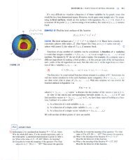
4. Applications to polar coordinates
For simplicity we consider a single nonlinear Schrödinger equation
−Δu − λu + Vu+ μu 3 = 0 in Ω,
u = 0 on Ω, (4.1)
where Ω={(x 1 ,x 2 ) ∈ R 2 : x1 2+x2 2 < 1} is the unit circle. Let x 1=r cos θ, x 2 =r sin θ, and set û(r, θ)=u(r cos θ,rsin θ).
Then (4.1) becomes
(
)
2 u
−
r 2 + 1 u
r r + 1 2 u
r 2 θ 2 − λu + Vu+ μu 3 = 0, 0

C.-S. Chien et al. / Journal of Computational and Applied Mathematics 214 (2008) 549 – 571 557
where we have dropped the “ ∧ ” sign in (4.2). We discretize (4.2) by the centered difference approximations described
in [17] with uniform mesh width Δr = 2/(2N + 1) on the radial direction and Δθ = 2π/M on the azimuthal direction
for some positive integers M and N. The locations of grid points are half integered in the radial direction and integered
in the azimuthal direction, i.e.,
r i = (i − 1 2 )Δr, θ j = (j − 1)Δθ, i = 1, 2,...,N + 1, j= 1, 2,...,M + 1.
Let U ij = u(r i , θ j ). Then the centered difference analogue of (4.2) is
−
(
Ui+1,j − 2U ij + U i−1,j
(Δr) 2
+ 1 r i
U i+1,j − U i−1,j
2Δr
+ 1
r 2 i
)
U i,j+1 − 2U ij + U i,j−1
(Δθ) 2
− λU ij + VU ij + μU 3 ij = 0
inΩ,
U N+1,j = 0 onΩ. (4.3)
Since u(r, θ) is 2π periodic in θ, wehaveU i,0 = U i,M and U i,1 = U i,M+1 . We can order the grid points either in the
radial direction or in the azimuthal direction. In both cases we obtain two nonsymmetric but similar matrices. We refer
to [7] for details.
The derivation of two-grid discretization schemes for (4.1) is the same as those given in Section 2 and is omitted
here. In conclusion, suppose that Δ˜r is the radial meshsize on the coarse grid. To avoid the singularity at the origin, we
have to choose Δr = (1/3 n )Δ˜r for some positive integer n as the radial meshsize on the fine grid.
5. Discrete systems
5.1. TCNLS
Eq. (1.4) can be expressed as
[ ]
−Δu1 + f(u
F(u 1 ,u 2 , λ 1 , λ 2 ) =
1 ,u 2 , λ 1 )
= 0. (5.1)
−Δu 2 + g(u 1 ,u 2 , λ 2 )
Let u = (u 1 ,u 2 ), C 2 0 (Ω) := {u ∈ C2 (Ω) | u| Ω = 0}, and X = (C 2 0 (Ω))2 , Y = (C 0 (Ω)) 2 . Then F : X × R 2 → Y is a
smooth mapping. Note that u 0 = (0, 0) is a trivial solution of (5.1) for all λ ∈ R 2 . Differentiating F with respect to u
at the homogeneous equilibrium u 0 = (0, 0), we obtain the linearization L of F , namely,
⎡
−Δ + f (0, λ 1 )
⎢ u
L := D u F(u 0 , λ 1 , λ 2 ) = ⎣
1
g
(0, λ 2 )
u 1
[
−Δ − λ1 I 0
=
0 −Δ − λ 2 I
⎤
⎥
⎦
(0, λ 2 )
u 2
]
, (5.2)
f
(0, λ 1 )
u 2
−Δ + g
where L : X × R 2 → Y . We discretize (5.1) by the centered difference approximations with uniform meshsize
h = 1/(N + 1) on the x- and y-axis. The centered difference analogue of (5.1) can be expressed as
{
A1 U − λ
F(U,V,λ 1 , λ 2 ) =
1 U + μ 1 U 3 + βV 2 ◦ U = 0,
A 1 V − λ 2 V + μ 2 U 3 + βU 2 ◦ V = 0.
(5.3)
Here A 1 ∈ R N 2 ×N 2 is the coefficient matrix associated with the discretization of the Laplacian −Δ, U =[U 1 ,U 2 ,...,
U N 2] T , V =[V 1 ,V 2 ,...,V N 2] T with h=1/(N +1) on the x- and y-axis, U ◦V =[U 1 V 1 ,U 2 V 2 ,...,U N 2V N 2] denotes
the Hadamard product of U and V , and U r =U ◦···◦U, the r-times Hadamard products of U. We denote X =[U,V] T

558 C.-S. Chien et al. / Journal of Computational and Applied Mathematics 214 (2008) 549 – 571
and treat λ 1 as the continuation parameter by varying the values of λ 2 and β. Note that F : R M × R → R M is a smooth
mapping with M =2N 2 . For convenience we fix λ 2 . Let the Jacobian matrix of F be denoted by DF =[D X F,D λ1 F ]∈
R (M+1)×M .Wehave
[
A1 + diag(−λ
D X F =
1 + 3μ 1 U 2 + βV 2 ]
) diag(2βV ◦ U)
diag(2βU ◦ V) A 1 + diag(−λ 2 + 3μ 2 V 2 + βU 2 )
and
[
−U
D λ1 F =
0
]
. (5.4)
Note that A 1 is symmetric and positive definite, and D X F is symmetric. The discrete operator corresponding to the
linear operator L in (5.2) is denoted by
[ ]
A1 − λ
A = 1 I 0
∈ R M×M . (5.5)
0 A 1 − λ 2 I
The eigenvalues and corresponding eigenvectors of A 1 are
(
)
λ p,q = 4(N + 1) 2 sin 2 pπ
2(N + 1) + qπ
sin2 , 1p, q N,
2(N + 1)
U p,q (x j ,y k ) = sin
jpπ
N + 1 sin kqπ
N + 1 . (5.6)
We can fix λ 2 so that the matrix A in (5.5) becomes singular if λ 1 = λ p,q . Thus the bifurcation point of the discrete
two-coupled nonlinear Schrödinger equations occur on the trivial solution curve at {(U, V, λ 1 ) = (0, 0, λ p,q ) | p, q =
1, 2,...,N}.
5.2. The Brusselator
The Brusselator is governed by
u
t = d 1Δu + f (u, v, λ) = d 1 Δu − (λ + 1)u + u 2 v + α in Ω =[0,l]×[0, 1],
v
t = d 2Δv + g(u, v, λ) = d 2 Δv + λu − u 2 v in Ω =[0,l]×[0, 1],
u(x,y,t)= α,
v(x,y,t)= λ α
on Ω. (5.7)
Eq. (5.7) has a uniform steady state solution (u 0 ,v 0 ) = (α, λ/α). We treat λ as the bifurcation parameter and fix α. Let
u = (u, v). Shifting u 0 = (α, λ/α) to u 0 = (0, 0), we obtain
f(u, λ) = (λ − 1)u + α 2 v + ((λ/α)u 2 + 2αuv + u 2 v),
g(u, λ) =−λu − α 2 v − ((λ/α)u 2 + 2αuv + u 2 v). (5.8)
Thus the steady state equations of (5.7) can be expressed as
[ ]
d1 Δu + f(u, λ)
F(u, λ) =
= 0, (5.9)
d 2 Δv + g(u, λ)

C.-S. Chien et al. / Journal of Computational and Applied Mathematics 214 (2008) 549 – 571 559
3 4
1
2
Fig. 1. An Adini’s element □ ij .
Table 1
The total execution time (in seconds) and total number of iterations on the fine gird for tracing the solution branch of (6.1) bifurcating at (0, λ ∗ 1,1 )
by implementing Methods 1, 2, 4 with six-node triangular elements
Method 1 Method 2 Method 4
(a) μ = 30
Time(s) 2489.22 2105.08 3799.11
Total Newton iterations 13 0 99
Total linear systems 126 100 198
Total Lanczos iterations 94581 79704 144723
(b) μ =−30
Time(s) 2495.63 2139.39 3867.81
Total Newton iterations 13 0 99
Total linear systems 126 100 198
Total Lanczos iterations 94765 81033 147127
where f(u, λ) and g(u, λ) are defined as in (5.8). Differentiating F with respect to u at the homogeneous equilibrium
u 0 = (0, 0), we obtain the linearization L of F with
⎡
d 1 Δ + f f ⎤
(0, λ) (0, λ)
⎢ u v ⎥
L := D u F(0, λ) = ⎣ g
(0, λ)
u d 2Δ + g ⎦
v (0, λ)
[
d1 Δ + (λ − 1)I α
=
2 ]
I
−λI d 2 Δ − α 2 . (5.10)
I
To simplify our computations, we choose l = 1. The centered difference analogue of (5.10) is given by
[
−d1 A
A = 1 + (λ − 1)I α 2 ]
I
−λI −d 2 A 1 − α 2 , (5.11)
I
where A 1 is defined as in (5.4). Let λ p,q be defined as in (5.6). Similar to the discussion given in [9,11], the eigenvalues
λ ∗ p,q of A are determined by those of the 2 × 2 matrices
[ −d1 λ p,q + (λ ∗ ]
p,q − 1) α2
B p,q =
−λ ∗ p,q −d 2 λ p,q − α 2 , p,q = 1,...,N.
Since det B p,q = d 1 d 2 λ 2 p,q − (d 2λ ∗ p,q − d 2 − α 2 d 1 )λ p,q + α 2 = 0, therefore
( ) 1 α
λ ∗ 2
p,q = d 1λ p,q + + d 1 + 1, p,q = 1,...,N. (5.12)
λ p,q d 2
Thus the bifurcation points of the Brusselator occur on the trivial solution curve at {(0, 0, λ ∗ p,q ) | p, q = 1,...,N},
where λ ∗ p,q are defined in (5.12).

560 C.-S. Chien et al. / Journal of Computational and Applied Mathematics 214 (2008) 549 – 571
0.9
0.6
μ=30
μ=−30
0.3
U(0.5,0.5)
0
−0.3
−0.6
−0.9
10 15 20 25 30
Fig. 2. The first solution branches of (6.1) with μ = 30 and μ =−30, respectively.
λ
Table 2
Locations of the first bifurcation points of (6.1)
Method Meshsize Matrix order Bifurcation (0, λ h ) |λ h − λ ∗ h | Time(s)
Triangular elements h = 64 1
4225 × 4225 (0, 20.02088404) 4.40 × 10 −4 129.95
Triangular elements h = 128 1
16641 × 16641 (0, 20.02090534) 4.19 × 10 −4 924.77
Triangular elements h = 256 1
66049 × 66049 (0, 20.02093030) 3.94 × 10 −4 6637.56
Adini’s elements h = 32 1
3267 × 3267 (0, 20.02091925) 4.05 × 10 −4 198.13
Two-grid solution (0, λ ∗ h ) = (0, 20.02132439)
Table 3
The total execution time (in seconds) and total number of iterations on the fine gird for tracing the solution branch of (1.4) bifurcating at (0, 0, λ 1,1 )
by implementing Methods 1–4 and the single-grid continuation method, V 1 = V 2 = 0, μ 1 = 10, μ 2 = 5, λ 2 = 30, β = 300, and Ω = (0, 1) 2
Method 1 Method 2 Method 3 Method 4 Single-grid
Time(s) 552.48 350.73 630.69 542.95 769.33
Total Newton iterations 53 12 99 99 118
Total linear systems 206 124 298 198 336
Total preconditioned Lanczos iterations 18111 11438 20695 17983 25248
5.3. The Adini elements
Let the domain S be split into small rectangles □ ij , i.e., S =∪ ij □ ij . Denote by h i and k j the boundary lengths of
□ ij , and h = max i,j {h i ,k j }. The rectangles □ ij are said to be quasiuniform if
h
min i,j {h i ,k j } c
for some constant c. The quasiuniform elements are said to be uniform if h i = h and k j = k. Without loss of generality
we may assume hk. Let V A ⊂ H0 1 (Ω) be the finite dimensional subspace spanned by the Adini elements,
V A ={v ∈ H 1 0 (S) : v|□ ij ∈ ̂P 3 ,v x and v y are continuous at all vertices of □ ij },

C.-S. Chien et al. / Journal of Computational and Applied Mathematics 214 (2008) 549 – 571 561
1
u 1 (0.5,0.5), u 2 (0.5,0.5)
0.8
0.6
0.4
u 1 , β=−300
u 2 , β=−300
u 1 , β=−600
0.2 u 2 , β=−600
u 1 , β=−900
u 2 , β=−900
0
−50 −40 −30 −20 −10 0 10 20 30
λ1
Fig. 3. The solution curves of u 1 and u 2 of (1.4) with V 1 = V 2 = 0, μ 1 = 10, μ 2 = 5, λ 2 = 30, and β =−300, −600, −900.
u 1 (0.5,0.5), u 2 (0.5,0.5)
0.45
0.4
0.35
0.3
0.25
0.2
0.15
0.1
0.05
u 1 , β=300
u 2 , β=300
u 1 , β=600
u 2 , β=600
u 1 , β=900
u 2 , β=900
0
15 20 25 30 35 40 45
Fig. 4. The solution curves of u 1 and u 2 of (1.4) with V 1 = V 2 = 0, μ 1 = 10, μ 2 = 5, λ 2 = 30, and β = 300, 600, 900.
λ 1
where
̂P 3 = span{1,x,y,x 2 ,y 2 ,xy,x 3 ,y 3 ,x 2 y,xy 2 ,x 3 y,xy 3 }. (5.13)
Note that the Adini elements are conforming for Poisson’s equation but not for biharmonic equations.
Denote □ ij ={(x, y) : x i x x i+1 ,y j y y j+1 }. We choose the affine transformations ξ = (x − x i )/h i and
η = (y − y j )/k j , where h i = x i+1 − x i and k j = y j+1 − y j . The admissible functions for the Adini elements are given
by
v(x,y) =
4∑
v l l (ξ, η) + h i
l=1
4∑
4∑
(v x ) l ψ l (ξ, η) + k j (v y ) l θ l (ξ, η). (5.14)
l=1
l=1

562 C.-S. Chien et al. / Journal of Computational and Applied Mathematics 214 (2008) 549 – 571
Fig. 5. The contours of the solutions u 1 and u 2 of (1.4) with V 1 =V 2 =0, μ 1 =10, μ 2 =5, λ 2 =30, and β=−300 at λ 1 =22.7315546, −94.0162850,
−396.206293, −2947.69410, respectively: (a) λ 1 = 22.7315546, (b) λ 1 =−94.0162850, (c) λ 1 =−396.206293, (d) λ 1 =−2947.69410.
where the nodal points 1, 2, 3, 4 denote the coordinates (i, j), (i + 1,j), (i, j + 1), and (i + 1,j + 1), respectively.
See Fig. 1
.
The 12 basis functions on S =[0, 1] 2 are given explicitly by
1 (x, y) = (1 − x)(1 − y)(1 + x + y − 2x 2 − 2y 2 ),
2 (x, y) = x(1 − y)(3x + y − 2x 2 − 2y 2 ),
3 (x, y) = (1 − x)y(x + 3y − 2x 2 − 2y 2 ),

C.-S. Chien et al. / Journal of Computational and Applied Mathematics 214 (2008) 549 – 571 563
Table 4
The total execution time (in seconds) and total number of iterations on the fine gird for tracing the first solution branch of (1.4) defined on the unit
circle by implementing Methods 1, 2, 4, and the single-grid continuation method, V 1 = (x 2 1 + x2 2 )/2, V 2 = (x 2 1 + x2 2 )/5, μ 1 = 10, μ 2 = 5, λ 2 = 10,
and β = 300.
Method 1 Method 2 Method 4 Single-grid
Time(s) 178.92 114.92 182.18 249.15
Total Newton iterations 39 14 110 201
Total linear systems 178 128 220 402
Total Bi-CGSTAB iterations 65975 43864 70560 95803
where
4 (x, y) = xy(−1 + 3x + 3y − 2x 2 − 2y 2 ),
5 (x, y) = ψ 1 (x, y) = (1 − y)̂ψ 0 (x),
6 (x, y) = ψ 2 (x, y) = (1 − y)̂ψ 1 (x),
7 (x, y) = ψ 3 (x, y) = ŷψ 0 (x),
8 (x, y) = ψ 4 (x, y) = ŷψ 1 (y),
9 (x, y) = θ 1 (x, y) = (1 − x)̂ψ 0 (y),
10 (x, y) = θ 2 (x, y) = x̂ψ 0 (y),
11 (x, y) = θ 3 (x, y) = (1 − x)̂ψ 1 (y),
12 (x, y) = θ 4 (x, y) = x̂ψ 1 (y), (5.15)
̂ψ0 (s) = s 3 − 2s 2 + s, ̂ψ1 (s) = s 3 − s 2 (5.16)
are the cubic Hermite basis functions on [0, 1].
6. Numerical results
The numerical algorithms described in Section 3 were implemented to traced solution branches of the TCNLS,
where ˜h =
16 1 and h = 256 1 . For convenience we denote Algorithm 3.1 and the three variants of Algorithm 3.1, i.e.,
replacing Step 2(ii) of Algorithm 3.1 by the corrector procedures (ii-1)–(ii-3) as Methods 1–4, respectively. The
TCNLS were discretized by the centered difference approximation with uniform meshsize on the x- and y-axis for
the rectangular domains Ω = (0, 1) 2 and (−6, 6) × (−6, 6), and on the radial- and azimuthal-direction for the unit
disk. We also compare the performance of six-node triangular elements and the Adini elements on a single grid. As
a side application Algorithm 3.1 was also implemented to trace solution branches of the Brusselator. The accuracy
tolerances for the linear solvers and the Newton corrector are 5 × 10 −10 and 5 × 10 −8 , respectively. All computations
were executed on a Pentium 4 computer using FORTRAN 95 Language with double precision arithmetic. In
these examples we computed 100 approximating points on the solution curves branching from the first bifurcation
points.
Example 1 (A single NLS). We consider a single NLS
−Δu(x) + V (x)u(x) + μ|u(x)| 2 u(x) = λu(x), x ∈ Ω = (0, 1) 2 ,
u(x) = 0, x ∈ Ω, (6.1)
where V(x)=
2 1 (x2 1 + x2 2 ). To start with, we used a two-grid finite element discretization scheme with ˜h =
16 1 and
h =
256 1 to compute the first eigenpair of the linear Schrödinger eigenvalue problem
−Δu(x) + V (x)u(x) = λu(x), x ∈ Ω,

564 C.-S. Chien et al. / Journal of Computational and Applied Mathematics 214 (2008) 549 – 571
Fig. 6. The contours of the solutions u 1 and u 2 of (1.4) with V 1 = (x 2 1 + x2 2 )/2, V 2 = (x 2 1 + x2 2 )/5, μ 1 = 10, μ 2 = 5, λ 2 = 10, and β = 300 at
λ 1 = 5.75096348, 16.4065407, 23.0804876, 73.0623656, respectively: (a) λ 1 = 5.75096348, (b) λ 1 = 16.4065407, (c) λ 1 = f , (d) λ 1 = 73.0623656.
u(x) = 0, x ∈ Ω. (6.2)
The first discrete eigenvalue of (6.2) on the fine grid is λ ∗ h = 20.02132439, where the residual norm is 10−9 . Next,
we used the two-grid six-node triangular discretization scheme to trace the solution curve of (6.1) branching from the
first bifurcation point (0, λ ∗ h ) ≈ (0, 20.02132439), where Methods 1, 2, and 4 were implemented with the Lanczos
method as the linear solver. Table 1 lists the total execution time as well as the total Lanczos and Newton iterations.
Fig. 2 displays the first solution branches of (6.1) with μ = 30 and μ =−30, respectively. Both the six-node triangular
elements and the Adini elements were also implemented on a single grid to trace the first solution branch of (6.1).
Table 2 lists the locations of the detected bifurcation points (0, λ h ) with various grid sizes.

C.-S. Chien et al. / Journal of Computational and Applied Mathematics 214 (2008) 549 – 571 565
Fig. 7. The contours of the solutions u 1 and u 2 of (1.4) with V 1 = (x 2 1 + x2 2 )/2, V 2 = (x 2 1 + x2 2 )/5, μ 1 = 10, μ 2 = 5, λ 2 = 25, and β =−300 at
λ 1 = 5.84931608, −1.01785437, −112.638902, −1490.83931, respectively: (a) λ 1 = 5.84931608, (b) λ 1 =−1.01785437, (c) λ 1 =−112.638902,
(d) λ 1 =−1490.83931.
Example 2 (TCNLS on the unit square). We chose V 1 = V 2 = 0, μ 1 = 10, μ 2 = 5 and λ 2 = 30 in (1.4), and treated
λ 1 as the continuation parameter. Table 3 lists the total execution time as well as the total preconditioned Lanczos and
Newton iterations, where Methods 1–4 and the single-grid continuation method were implemented to trace the first
solution branch. Fig. 3 shows that the solution curves of u 1 and u 2 are pitchfork and subcritical, where β=−300, −600
and −900. That is, the solution curves turn to the left of the bifurcation point. Fig. 4 shows that the solution curves of
u 1 and u 2 are pitchfork and supercritical, where β = 300, 600 and 900. The contours of the solution curves of u 1 and
u 2 with β =−300 at λ 1 = 22.7315546, −94.0162850, −396.206293, and −2947.69410 are displayed in Fig. 5.

566 C.-S. Chien et al. / Journal of Computational and Applied Mathematics 214 (2008) 549 – 571
Fig. 8. The contours of the real and imaginary parts of the wave solutions Φ j , j = 1, 2 with λ 1 =−1490.83931, λ 2 = 25.0, respectively, at t = 100.
0.6
0.5
||u 1 || ∞ , ||u 2 || ∞
0.4
0.3
0.2
0.1
0
0 2 4 6 8 10 12 14
λ 1
u 1
u 2
Fig. 9. The solution curves of u 1 and u 2 of (1.4) with Ω = (−6, 6) 2 , V 1 = (x 2 1 + x2 2 )/2, V 2 = (x 2 1 + x2 2 )/5, μ 1 = 10, μ 2 = 5, λ 2 = 2.5, and β = 300.
Example 3 (TCNLS on the unit circle). We study the two-coupled NLS as in (1.4), where V 1 = (x 2 1 + x2 2 )/2, V 2 =
(x 2 1 + x2 2 )/5, μ 1 = 10, μ 2 = 5, λ 2 = 10 or 25, β = 300 or −300, and treated λ 1 as the continuation parameter. In
Table 4 we list the total execution time as well as the total Bi-CGSTAB and Newton iterations, where Methods 1, 2,
4, and the single-grid continuation method were implemented to trace the first solution branch. We observe that the
two-grid methods are better than the single-grid method and Method 2 is superior to the other two two-grid methods.
The contours of the solution curves of u 1 and u 2 with λ 2 =10 and β=300 at λ 1 =5.75096348, 16.4065407, 23.0804876,
and 73.0623656 are displayed in Fig. 6. The contours of the solution curves of u 1 and u 2 with λ 2 = 25 and β =−300

C.-S. Chien et al. / Journal of Computational and Applied Mathematics 214 (2008) 549 – 571 567
Fig. 10. The contours of the solutions u 1 and u 2 of (1.4) with Ω = (−6, 6) 2 , V 1 = (x 2 1 + x2 2 )/2, V 2 = (x 2 1 + x2 2 )/5, μ 1 = 10, μ 2 = 5, λ 2 = 2.5, and
β = 300 at λ 1 = 1.61545937, 2.41149804, 4.59511622, 13.0373400, respectively: (a) λ 1 = 1.61545937, (b) λ 1 = 2.41149804, (c) λ 1 = 4.59511622,
(d) λ 1 = 13.0373400.
at λ 1 = 5.84931608, −1.01785437, −112.638902, and −1490.83931 are displayed in Fig. 7. Fig. 8 displays the wave
functions Φ 1 and Φ 2 at λ 1 =−1490.83931, λ 2 = 25, and t = 100.
Example 4 (TCNLS on the square Ω = (−l, l) 2 ). We study the two-coupled NLS (1.4) defined on Ω = (−l, l) 2 ,
where l = 6, V 1 = (x 2 1 + x2 2 )/2, V 2 = (x 2 1 + x2 2 )/5, μ 1 = 10, μ 2 = 5, λ 2 = 2.5, β = 300, and treated λ 1 as the
continuation parameter. Methods 1–4 were implemented to traced solution branches of this example, where we chose

568 C.-S. Chien et al. / Journal of Computational and Applied Mathematics 214 (2008) 549 – 571
100
80
λ ∗ 1,1
60
40
20
(0.5, 54.3601204)
(1, 37.5495407)
(3, 26.3424876)
(2, 29.1442509)
(4, 24.941606)
0
0 2 4 6 8
d 2
Fig. 11. The bifurcation curve of (5.9) with d 1 = 1, α = 4, h = 1
256 .
Table 5
The total execution time (in seconds) and total number of iterations on the fine gird for tracing the solution branch of (5.9) bifurcating at (0, 0, λ ∗ 1,1 )
Method 1 Method 2 Method 3 Method 4 Single-grid
(a) Right solution branch of u and v
Time(s) 3565.23 1249.34 2328.91 2494.53 3732.38
Total Newton iterations 96 0 90 99 104
Total linear systems 292 100 280 198 308
Total Bi-CGSTAB iterations 152226 53377 99149 106447 158853
(b) Left solution branch of u and v
Time(s) 3739.50 3046.36 2529.66 2567.72 3838.73
Total Newton iterations 98 89 95 99 102
Total linear systems 296 278 290 198 304
Total Bi-CGSTAB iterations 160010 130093 107694 109710 163867
2.5
2
U
V
1.5
U(0.5,0.5), V(0.5,0.5)
1
0.5
0
−0.5
−1
−1.5
−2
26 28 30 32 34 36 38
λ
Fig. 12. The solution curves of u and v branching from the first bifurcation point (0, 0, λ ∗ 1,1 ) of (5.9) with d 1 = 1, d 2 = 2, α 2 = 4, and l = 1.

C.-S. Chien et al. / Journal of Computational and Applied Mathematics 214 (2008) 549 – 571 569
Fig. 13. The contours of the solutions u and v of (5.9) with d 1 = 1, d 2 = 2, α = 4, and l = 1 at: (a) λ = 26.7036738, (b) λ = 30.0809857, (c)
λ = 228.491101, respectively.
˜h = 2l/32 and h = 2l/256. The first discrete bifurcation points on the coarse and fine grids are (u 1 ,u 2 , λ 1 ) ≈
(0, 0, 1.40536883) and (0, 0, 1.41407622), respectively. Fig. 9 shows the first solution branches of u 1 and u 2 . The
contours of the solution curves of u 1 and u 2 at λ 1 = 1.61545937, 2.41149804, 4.59511622, and 13.0373400 are
displayed in Fig. 10.
Example 5 (The Brusselator). In this example, we chose l = 1, d 1 = 1, d 2 = 2 and α = 4 in (5.9).The first bifurcation
point on the trivial solution curve is (u, v, λ) ≈ (0, 0, 29.1444935367).Forh =
256 1 , the first discrete bifurcation point
is (U, V, λ ∗ 1,1 ) = (0, 0, 29.1442509002). Fig. 11 displays the bifurcation curve for various values of d 2 with d 1 = 1,
α = 4, h =
256 1 . In our numerical experiments, Methods 1–4 and the single-grid continuation method were implemented
to trace the solution curve branching from the first bifurcation point (0, 0, λ ∗ 1,1 ), where the Bi-CGSTAB method [23]
was used as the linear solver. Table 5 lists the total execution time, the total Bi-CGSTAB iterations, and the Newton
iterations on the fine grid. Fig. 12 shows that the solution curves of u and v branching from (0, 0, λ ∗ 1,1 ) are transcritical.
The contours of the solution curves of u and v at λ = 26.7036738, 30.0809857, 228.491101 are displayed in Fig. 13.

570 C.-S. Chien et al. / Journal of Computational and Applied Mathematics 214 (2008) 549 – 571
7. Conclusions
We have presented efficient two-grid discretization schemes with two-loop continuation algorithms for computing
wave functions of nonlinear Schrödinger equations. Some variants of the correct procedure in the inner continuation are
also proposed. Both rectangular and polar coordinates are considered in our numerical experiments. As a comparison
the six-node triangular elements and the higher order Adini elements are also exploited to discretize a single NLS. Our
numerical result shows that it is very promising to develop two-grid discretization schemes using the Adini elements
when the domain is rectangular. The two-grid discretization schemes we discussed in this paper also can be used to
compute stationary solutions of reaction–diffusion systems.
Based on the numerical results reported in Section 6, we wish to give some conclusions concerning the performance
of the algorithms we proposed in Section 3.
1. The main costs of the proposed algorithms depend on: (i) how many linear systems are required to be solved on
the fine grid and (ii) how close are the initial guesses to the exact solution curves. In case (ii) we can see, e.g., from
Tables 1,3,4, and 5a that most initial guesses for Newton’s method in Method 2 can be accepted as approximating
points for the solution curve c on the fine grid.
2. Implementing Algorithm 3.1 for Examples 2–5 is only slightly cheaper than implementing the continuation algorithm
on a single fine grid.
3. Finally, we conclude that it is unnecessary to perform quadratic approximations for computing stationary solutions
of reaction–diffusion systems.
References
[1] J.R. Anglin, W. Ketterle, Bose–Einstein condensation of atomic gases, Nature 416 (2002) 211–218.
[2] W. Bao, Ground states and dynamics of multicomponent Bose–Einstein condensates, Multiscale Model. Simul. 2 (2004) 210–236.
[3] W. Bao, Q. Du, Computing the ground state solution of Bose–Einstein condensates by a normalized gradient flow, SIAM J. Sci. Comput. 25
(2004) 1674–1697.
[4] W. Bao, D. Jacksch, P.A. Markowich, Numerical solution of the Gross-Pitaevskii equation for Bose–Einstein condensation, J. Comput. Phys.
187 (2003) 318–342.
[5] W. Bao, S. Jin, P.A. Markowich, Numerical study of time-splitting spectral discretizations of nonlinear Schrödinger equations in the semiclassical
regimes, SIAM J. Sci. Comput. 25 (2003) 27–64.
[6] S.-L. Chang, C.-S. Chien, B.-W. Jeng, Liapunov–Schmidt reduction and continuation for nonlinear Schrödinger equations, SIAM J. Sci. Comput.
29 (2007) 729–755.
[7] S.-L. Chang, C.-S. Chien, B.-W. Jeng, Computing wave functions of nonlinear Schrödinger equations: a time-independent approach, J. Comput.
Phys. (2007), in press, doi:10.1016/j.jcp.2007.03.028.
[8] Y. Chen, Y. Huang, D. Yu, A two-grid method for expanded mixed finite-element solution of semilinear reaction–diffusion equations, Internat.
J. Numer. Methods Eng. 57 (2003) 193–209.
[9] C.-S. Chien, M.-H. Chen, Multiple bifurcations in a reaction–diffusion problem, Comput. Math. Appl. 35 (1998) 15–39.
[10] C.-S. Chien, B.-W. Jeng, A two-grid discretization scheme for semilinear elliptic eigenvalue problems, SIAM J. Sci. Comput. 27 (2006)
1287–1304.
[11] C.-S. Chien, Z. Mei, C.-L. Shen, Numerical continuation at double bifurcation points of a reaction–diffusion problem, Internat. J. Bifurcation
Chaos 8 (1998) 117–139.
[12] P. Ghosh, Exact results on the dynamics of two-component Bose–Einstein condensate, Phys. Rev. Lett. 85 (2000) 5030–5033.
[13] A. Gierer, H. Meinhardt, A theory of biological pattern formation, Kybernetik 12 (1972) 30–39.
[14] D.S. Hall, M.R. Matthews, J.R. Ensher, C.E. Wieman, E.A. Cornell, Dynamics of component separation in a binary mixture of Bose–Einstein
condensates, Phys. Rev. Lett. 81 (1998) 1539–1542.
[15] H.T. Huang, Z.C. Li, Global superconvergence of Adini’s elements coupled with the Trefftz method for singular problems, Eng. Anal. Boundary
Elem. 27 (2003) 227–240.
[16] H.T. Huang, Z.C. Li, N. Yan, New error estimates of Adini’s elements for Poisson’s equation, Appl. Numer. Math. 50 (2004) 49–74.
[17] M.-C. Lai, A note on finite difference discretizations for Poisson equation on a disk, Numer. Methods Partial Differential Equations 17 (2001)
199–203.
[18] T.-C. Lin, J. Wei, Ground state of N coupled nonlinear Schrödinger equations in R n , n3, Comm. Math. Phys. 255 (2005) 629–653.
[19] J.D. Murray, Mathematical Biology, Springer, Berlin, 1989.
[20] C.J. Myatt, E.A. Burt, R.W. Ghrist, E.A. Cornell, C.E. Wieman, Production of two overlapping Bose–Einstein condensates by sympathetic
cooling, Phys. Rev. Lett. 78 (1997) 586–589.
[21] W.-M. Ni, Qualitative properties of solutions to elliptic problems, in: M. Chipot, P. Quittner (Eds.), Handbook of Differential Equations, vol.
I, Stationary Partial Differential Equations, North-Holland, Amsterdam, 2004, pp. 157–233.

C.-S. Chien et al. / Journal of Computational and Applied Mathematics 214 (2008) 549 – 571 571
[22] I. Prigogine, R. Lefever, Stability and self-organization in open systems, in: G. Nicolis, R. Lefever (Eds.), Membranes, Dissipative Structures,
and Evolution, Benjamin, New York, 1974, pp. 1–16.
[23] H.A. van der Vorst, Bi-CGSTAB: a fast and smoothly converging variant of Bi-CG for the solution of nonsymmetric linear systems, SIAM J.
Sci. Statist. Comput. 13 (1992) 631–644.
[24] L. Wu, M.B. Allen, A two-grid method for mixed finite-element solution of reaction–diffusion equations, Numer. Methods Partial Differential
Equations 15 (1999) 317–332.
[25] L. Wu, M.B. Allen, Two-grid methods for mixed finite-element solution of coupled reaction–diffusion systems, Numer. Methods Partial
Differential Equations 15 (1999) 589–604.