Seismic Inversion - The Rice Inversion Project - Rice University

university-logo 

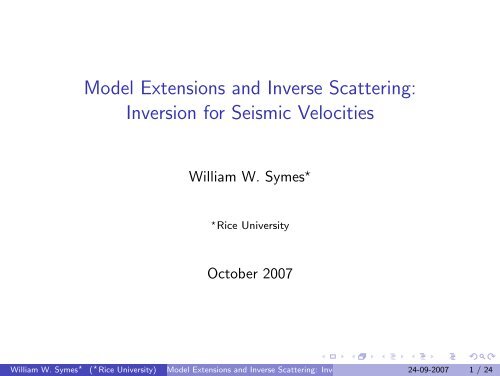
Model Extensions and Inverse Scattering: 

Inversion for Seismic Velocities 

William W. Symes ⋆ 

⋆ Rice University 

October 2007 

William W. Symes ⋆ ( ⋆ Rice University) Model Extensions and Inverse Scattering: Inversion for Seismic Velocities 24-09-2007 1 / 24


Expanded version of presentation in “Recent Advances and Road Ahead” 

session, SEG 2007. 

References to related SEG 07 talks in red - available via Scitation, 

www.seg.org. 

PDF available at www.trip.caam.rice.edu. 

Draft paper with references: www.caam.rice.edu, TR 07-05. 


Introduction 

Focus: recent developments in waveform inversion (WI) for velocity, and 

relation to migration velocity analysis (MVA). 

Main topics: 

Why inversion via least squares data fitting (“waveform inversion”) 

doesn’t work for exploration seismology; 

How migration is an approximate solution of the linearized inverse 

problem; 

How “Kirchhoff” and “Wave Equation” prestack depth migration 

differ, and what that means for migration velocity analysis; 

How to formulate migration velocity analysis via optimization, use all 

events; 

How to view migration velocity analysis as a solution of a “partly 

linear” waveform inversion problem; 

How nonlinear waveform inversion might be integrated with migration 

velocity analysis. 



Marine Seismic Reflection Experiment 

Airguns = source of sound. Streamer consists of hydrophone receiver 

groups. Each group records a trace (time series of pressure) for each shot 

= excitation of source. Source-receiver distance = offset. 




Typical Shot Record 

time (s) 

0 

0.5 

1.0 

1.5 

2.0 

offset (km) 

0.5 1.0 1.5 

CMP gather from North Sea Survey 

(thanks: Shell). 

Processing applied: 

bandpass filter 3-8-25-35 Hz; 

cutoff or mute to remove 

non-reflection energy (direct, 

diving, head waves); 

predictive deconvolution to 

suppress multiple reflections. 


Mechanical properties of sedimentary rocks 

v p varies significantly. 

Heterogeneity at all scales - km 

to mm to µm. 

Well (v p) log from Texas borehole 

(thanks: P. Janak, Total E&P, USA) 



Point Source Acoustics - the minimal model 

Earth = Ω = R 3 . Wave equation for acoustic potential response to 

isotropic point radiator at x s , time dependence w(t): 

( 1 

v 2 ∂ 2 u 

∂t 2 − ∇2 ) 

u(t, x; x s ) = w(t)δ(x − x s ) 

plus initial and boundary conditions. 

Lions, late ’60’s: problem well posed for v ∈ A 0 = {log v ∈ L ∞ (Ω)}, RHS 

in L 2 ([0, T ] × Ω). 

Forward map: F : A 0 → L 2 (Σ × [0, T ]), Σ ⊂ {x 3 = 0} × {x 3 = 0} open, 

samples pressure: 

( 

F[v](t, x r ; x s ) = φ ∂u ) 

(t, x r ; x s ), (t, x r , x s ) ∈ [0, T ] × Σ, φ ∈ C0 

∞ (Σ) 

∂t 

If v = v 0 known & constant in {x 3 < z} for some z > 0, slight extension 

of Lions shows F well-defined. Stolk 2000: continuous, diffb’le 

“with loss of derivative”. 




Agenda 

1 Waveform Inversion 

2 Migration Velocity Analysis 

3 Semblance and Optimization 

4 Extended Modeling: MVA + WI 

5 Conclusions and Prospects 


Inversion Generalities 

The usual set-up: 

M = a set of models (v ∈ A 0 ); 

D = a Hilbert space of (potential) data (L 2 ([0, T ] × Σ)); 

F : M → D: modeling operator or “forward map”. 

Waveform inversion problem: given d ∈ D, find v ∈ M so that F[v] ≃ d. 

F can incorporate any physics - acoustics, elasticity, anisotropy, 

attenuation,.... (and v may be more than velocity...). 

Typical problem size for adequately sampled 3D survey simulation: 

dim(M) ∼ 10 10 , dim(D) ∼ 10 12 

⇒ any computational “solution” must admit algorithms that scale well 

with problem size - if iterative, then iteration count should be essentially 

independent of dimension. 



Output Least Squares Inversion 

Given d ∈ D, find v ∈ M to minimize 

J OLS (v, d) = 1 2 ‖d − F[v]‖2 ≡ 1 2 (d − F[v])T (d − F[v]) 

Has long and productive history in geophysics - but not in reflection 

seismology. 

Only Newton and relatives scale well - but these find only local minima. 

Unfortunately, J OLS has lots of local minima having nothing to do with 

“truth”, for typical length, time, and frequency scales of exploration 

seismology. 

⇒ least squares waveform inversion with Newton-like iteration “doesn’t 

work” (Gauthier 86, Kolb 86, Santosa & S. 89, Bunks 95, Shin 01, Shin 

and Min 06, many others - see Chung SI 2.4). 





Simple but instructive example: 1D reflection, v = v(z), wavefield is plane 

wave at normal incidence with wavelet w(t). 

At constant velocity v(z) ≡ v 0 , 

where ˇw(t) = w(−t). 

∇J OLS [v 0 ](z) = const. 

( d ˇw 

dt ∗ (d − w) ) ( 2z 

v 0 

) 

If data (hence w) contains no energy at frequencies below f min , then 

gradient contains no energy at spatial wavelengths longer than v 0 /(2f min ) 

⇒ first step of Newton does not even begin to reconstruct nonzero mean 

deviations if z d > v 0 /(4f min ). 



Upgrade to layered (or near-layered) media via plane wave expansion, 

range of incidence angles θ: v 0 → v 0 / cos θ. 

⇒ using reflection data with incidence angles ≤ 60 ◦ , gradient-based 

method cannot update mean velocity over depth interval [0, z d ] if 

f min > v 0 

2z d 

Typical shallow sediment imaging: v 0 ≃3 km/s, z d = 5 km ⇒ to recover 

nonzero mean deviation from 3 km/s must have significant energy at 

f min ≃ 0.3Hz (cf. Bunks 95, Chung SI 2.4, Pillet SI 4.5) 

If not present (energetics - Ziolkowski 93) and/or filtered from data, and if 

〈v〉 ≠ v 0 , then spurious minima must exist (and will be found by 

gradient-based optimization from v init = v 0 )! 




0 

midpoint (km) 

0 5 10 

0 

offset (km) 

0 0.1 0.2 0.3 0.4 0.5 

v (km/s) 

1.0 1.5 2.0 2.5 3.0 

0 

0.1 

0.1 

0.2 

depth (km) 

0.2 

0.3 

time (s) 

0.2 

0.3 

0.4 

depth (km) 

0.4 

0.6 

0.4 

0.5 

0.5 

0.6 

0.8 

0.6 

0.7 

1.0 

1.6 1.8 2.0 2.2 2.4 

km/s 

Left: Layered model. Middle: response to point source in center, 

4-10-30-40 Hz bandpass wavelet. Right: OLS inversions, dashed=initial, 

solid=final. Quasi-Newton iteration terminated when gradient reduced by 

10 −2 . 




Examples of successful waveform inversion from synthetic data containing 

very low frequencies (


Agenda 








The Seismologist’s Standard Model 

[Thanks: P. Lailly]. Because (1) F is hard to understand, (2) it’s a lot 

simpler, and (3) it works sometimes, assume separation of scales: v [and 

other mechanical parameters] superposition of: 

smooth macromodel v: the long-scale component of velocity etc. 

(scales ≃ 1 km and larger). 

oscillatory perturbation δv: high-frequency component of the velocity, 

scale ≃ 10’s of m (wavelength). 

( 1 ∂ 2 ) 

u 

v 2 ∂t 2 − ∇2 δu(t, x; x s ) = 2δv(x) ∂ 2 u 

v 3 (x) ∂t 2 (t, x; x s), DF[v]δv = ∂δu 

∣ 

∂t 

∣ 

[0,T ]×Σ 



Linearized Acoustic Inverse Problem 

v smooth, r oscillatory (or even singular): 

( 1 ∂ 2 ) 

u 

v 2 ∂t 2 − ∇2 δu(t, x; x s ) = 2δv(x) ∂ 2 u 

v 3 (x) ∂t 2 (t, x; x s), DF[v]δv = ∂δu 

∣ 

∂t 

Admissible sets of macromodels: bounded A ⊂ C ∞ (Ω),... 

Beylkin 85, Bleistein 87, Rakesh 88, Burridge 89, Nolan 97, de Hoop 97, 

ten Kroode 98, Stolk 00: under ever-weaker conditions, DF[v] ∗ DF[v] is 

(microlocally) invertible pseudodifferential operator. 

Means: DF[v] almost unitary, DF[v] ∗ (d − F[v]) has same 

(near-)singularities as δv, differs by scaling (S., SI 2.2) - image of δv. 

DF[v] ∗ = prestack depth migration operator. 

∣ 

[0,T ]×Σ 



Linearized Acoustic Inverse Problem 

Partially linearized inverse problem = Migration Velocity Analysis: given 

d ∈ D ≡ L 2 ([0, T ] × Σ), find v ∈ A, δv ∈ E ′ (Ω) so that 

DF[v]δv ≃ d − F[v]. 

Least squares approach no more successful than for basic IP. Instead, 

industry has developed migration velocity analysis methods. 

Based on image volume I output by prestack depth migration - function of 

subsurface position x and other (redundant) parameters. Two major 

variants: surface-oriented and depth-oriented. 

Recent advance: understanding the difference. 



Migration and Imaging Conditions 

(I) Surface oriented: diffraction sum representation of image volume 

I S (x, h) = ∑ m 

(...)d(m, h, T [v](x, m − h) + T [v](x, m + h)) 

where h = 0.5(x r − x s ) = half-offset, m = 0.5(x r + x s ) = midpoint, 

T (x, y) = one-way time from x to y. (...) = optional amplitude, 

antialiasing,.. Data with same h = offset bin. 

Relation is binwise: offset bin of image depends only on corresponding 

offset bin of data, hence “common offset”. Diffraction sum is only comp. 

feasible implementation, hence “Kirchhoff” migration. 

Other binwise migrations: common shot, common receiver, common 

scattering angle... 




(II) Depth oriented image volume: also has diffraction sum representation 

I D (x, H) = ∑ m 

∑ 

(...)d(m, h, T [v](x − H, m − h) + T [v](x + H, m + h)) 

h 

H is space shift or depth offset vector - unrelated to acquisition geometry. 

Note extra summation over h: every image value depends on all traces. 

Usual implementation via one-way WE (shot profile or DSR, Claerbout 85) 

or two-way RTM (Biondi-Shan 02, S. 02) (hence “wave equation” 

migration). 

Transform to scattering angle available - Prucha 99, Sava and Fomel 01. 

Time shift variant - Sava and Fomel 05. 



Imaging conditions: how to extract image from image volume. 

(I) Surface oriented: stack over offset 

I (x) = ∑ h 

I S (x, h) 

(II) Depth oriented: extract zero (depth) offset section 

I (x) = I D (x, 0) 

NB: These really are the same! In both cases, I ≃ DF[v] ∗ (d − F[v]) 

(high freq asymptotic approximation). 

So both variants produce same image... 





But not the same image volume! 

Nolan & S. 97, Stolk & S. 04, deHoop & Brandsberg-Dahl 03: 

multipathing (multiple rays connecting source, receiver, and image points, 

caustics) leads to artifacts in surface oriented image volume. 

Artifact = coherent event in wrong place, of strength comparable to 

correct events. 

Stolk & deHoop 01, S. 02, Stolk 05: depth-oriented image volume 

generally free of artifacts, even with strong multipathing. 

So the two types of image volume are not even kinematically equivalent! 

Accounts for perceived superiority of “wave equation migration”. 

Consequences for velociy analysis: Nolan and S. 97, Xu TOM 1.4. 



0 

x (km) 

2 4 6 8 

z (km) 

2 

1.0 1.5 2.0 2.5 

v (km/s) 

Velocity model after Valhall field, North Sea. Note sloping reflector at left, 

large low-velocity lens (modeling gas accumulation) in center. Both tend 

to produce multipathing. (Thanks: M. de Hoop, A. Malcolm) 




0 

x(km) 

2 4 6 8 

1 

t(s) 

2 

3 

4 

Typical shot gather over center of model, exhibiting extensive 

multipathing. 




0 

angle(deg) 

20 40 60 

angle(deg) 

0 20 40 60 

0 

0.5 

0.5 

z(km) 

1.0 

z(km) 

1.0 

1.5 

1.5 

2.0 

2.0 

Angle common image gathers at same horizontal position from 

surface-oriented (Kirchhoff) and depth-oriented (DSR) migrated image 

volumes. Left: ACIG from Kirchhoff migration: kinematic artifacts clearly 

visible. Right: ACIG from DSR migration: no artifacts! 




Agenda 








Semblance 

Semblance condition - complementary to imaging condition. 

Expresses consistency between data, velocity model in terms of image 

volume. 

(I) Surface oriented: velocity-data consistency when I S (x, h) independent 

of h (at least in terms of phase), i.e. image gathers are flat. 

(II) Depth oriented: velocity-data consistency when I D (x, H) concentrated 

near H = 0, i.e. image gathers are focused [or flat, when converted to 

scattering angle]. 


Semblance 

offset (km) 

-0.2 -0.1 0 0.1 

0 

offset (km) 

-0.2 -0.1 0 0.1 

0 

offset (km) 

-0.2 -0.1 0 0.1 

0 

0.1 

0.1 

0.1 

0.2 

0.2 

0.2 

depth (km) 

0.3 

depth (km) 

0.3 

depth (km) 

0.3 

0.4 

0.4 

0.4 

0.5 

0.5 

0.5 

OIG, x=1 km: vel 10% low 

Offset Image Gather, x=1 km 

OIG, x=1 km: vel 10% high 

Image gathers {I D (x, H) : x, y fixed, H = (0, h, 0)}, amplitude vs. (z, h), 

from velo model v 0 + δv, v 0 = const., δv = randomly distributed point 

diffractors. Left to Right: use v = 90%, 100%, 110% of true velocity v 0 . 




Semblance 

Leads to two methods for velocity updating: 

(I) Depth domain reflection traveltime tomography: 

(auto)pick events in migrated image volume 

backproject inconsistency (eg. residual moveout of angle gather 

events) to construct velocity update as in standard traveltime 

tomography. 

Used with both surface oriented and depth oriented image volume 

formation. 

Drawback: uses only small fraction of events in typical image volume. 


Semblance 

(II) Depth domain reflection waveform tomography (“differential 

semblance”): 

form measure of deviation of image volume from semblance condition 

- function of velocity model; all energy not conforming to semblance 

condition contributes. 

optimize numerically: gradient = backprojection of 

semblance-inconsistent energy into velocity update. 

Also used with both surface and depth oriented image volumes. Recent 

contributions: Shen 03, 05, Li & S. 05, Foss 06, Albertin 06, Khoury 06, 

Verm 06, Kabir SVIP 2.3. 

Inherently uses all events in data, weighted by strength. 

Example: minimize J[v] = ∑ |HI D (x, H)| 2 - penalizes energy at H ≠ 0. 



Synthetic Example (Shen SEG 05) 

Starting velocity model for waveform tomography. Data: Born version of 

Marmousi, fixed receiver spread across surface. 




Image (I D (x, H = 0)) at initial velocity. 




Final velocity (47 iterations of descent method). Note appearance of high 

velocity fault blocks. 




Image (I D (x, H = 0)) at final velocity. 




Field Example - Trinidad (Kabir SVIP 2.3) 

[see Expanded Abstract, SEG 07.] 



Agenda 








Extended Modeling 

Where we are: 

(i) WI lets you model any physics at all, and use all of the data, but 

doesn’t work (spurious local minima); 

(ii) MVA works - can even be made into an optimization without spurious 

local minima (“waveform tomography”, differential semblance) - but only 

produces velocity, and assumes linearized model (single scattering, Born 

approximation, primaries-only data,...). 

Can the two be combined somehow, while retaining their advantages? 




Partial Answer: MVA solves a version of WI! To see this, need extended 

modeling concept, plus true amplitude migration or linear inversion. 

Extended model ¯F : ¯M → D, where ¯M is a bigger model space. Physical 

model space M in 1-1 correspondence with a subset of ¯M, via extension 

map χ. 

For surface-oriented extended modeling, extended models depend on h, 

and χ[v](x, h) = v(x), i.e. χ produces models not depending on h. 

For depth-oriented extended modeling, extended models depend on H, and 

χ[v](x, H) = v(x)δ(H), i.e. χ produces models focused at zero offset. 

In either case, output of χ is an “image volume” satisfying the semblance 

condition, and vis-versa - which “explains” semblance condition. 



Lailly, Tarantola, Claerbout (80’s): migration operator (producing image) 

is adjoint or transpose DF[v] ∗ . True amplitude migration is 

(pseudo)inverse DF[v] −1 . 

Same relation with extended modeling: migration operator (producing 

image volume) is adjoint D ¯F[χ[v]] ∗ of linearized extended modeling 

operator. True amplitude migration defines (pseudo)inverse D ¯F[χ[v]] −1 . 

For depth orientation, diffraction sum representation is 

∫ 

= 

D ¯F[χ[v]]δ¯v(m, h, t) 

dxdHδ¯v(x, H)δ(t − T (x − H, m − h) − T (x + H, m + h)) 

Easy to check: D ¯F[χ[v]] T d(x, H) = I D (x, H). 





Claim: MVA (with true amplitude) solves “partially linearized” problem: 

find reference velocity v and perturbation δv so that DF[v]δv ≃ d − F[v]. 

Proof: successful MVA produces image volume satisfying imaging 

condition, i.e. I D = χ[δv]. 

Use true amplitude migration, and you get 

D ¯F[χ[v]] −1 (d − F[v]) ≃ χ[δv], whence 

Q.E.D. 

DF[v]δv = D ¯F[χ[v]]χ[δv] 

≃ D ¯F[χ[v]]D ¯F[χ[v]] −1 (d − F[v]) ≃ d − F[v] 




Linearization of what? 

Exercise for reader: for V = SAPD op on appropriate Hilbert space, define 

¯F[V ] ≡ ∂ū 

∣ 

[0,T ]×Σ 

, where 

∂t 

V −2 ∂2 2 ū 

− ∇ 2 ū = w(t)δ(x − x s ) 

∂t 

Suppose distribution kernel of V is v(x)δ ( ) ( 

x−¯x 

2 + δ¯v x+¯x 

2 , x−¯x ) 

2 , then 

D ¯F[χ[v]]δ¯v has diffraction sum representation given above: its adjoint is 

depth-oriented prestack migration! (H ∼ x−¯x 

2 ) 

Existence theory for symmetric hyperbolic systems with operator 

coefficients after Lions 68. 




So what? Well, 

In this scheme, F can be any modeling operator - acoustic, elastic, ... 

- known how to do true amplitude, thanks to Beylkin, Burridge, 

Bleistein, de Hoop,... So: MVA extended to elastic (Born) modeling, 

for instance. 

For depth-oriented extension, ¯F expresses action at a distance: elastic 

moduli are nonlocal, stress at x + H results from strain at x − H. So 

Claerbout’s semblance principle is actually Cauchy’s 

no-action-at-a-distance hypothesis! [Thanks: Scott Morton] 

Nonlinear MVA via enforcing semblance = no-action-at-distance on 

elastic moduli, treated as operators - MVA incorporating multiple 

scattering = WI with extended modeling. 



Agenda 







Conclusions 

Takeaway messages of this talk: 

Least squares WI prone to get trapped in useless local minima - 

avoidance requires either initial velocity estimates good to 0.5 

(shortest) wavelength, or longest wavelength exceeding the survey 

depth. 

MVA: “Kirchhoff” (surface-oriented) and “Wave Equation” 

(depth-oriented) prestack migrations have different kinematic 

properties. 

MVA via waveform tomography (“differential semblance”), based on 

semblance condition and numerical optimization, uses all events to 

constrain velocity updates, much less tendency towards local minima 

than least squares WI. 

MVA solves a “partially linearized” WI problem based on extended 

modeling - nonphysical degrees of freedom. 

Nonlinear extended scattering = framework for uniting MVA and 

waveform inversion. 




Prospects 

Two kinematically inequivalent extensions: surface-oriented and 

depth-oriented. Classify all extensions by microlocal equivalence. 

Waveform MVA via Reverse Time Migration (= full-blown 

computation of D ¯F[χ[v]] ∗ ) and differential semblance - kinematic 

accuracy, fast linear inversion (SI 2.2, Moghaddam SPMI 3.2). 

Concepts other than differential semblance, least squares: van 

Leeuwen SI 2.8. 

Nonlinear inversion via model extension (“nonlinear MVA”) including 

multiple scattering ⇒ sparse representation of operator coefficients, 

introduction of “control” (∼ migration velocity), integration of source 

estimation (Minkoff & S. 97). 



Thanks to 

Total E&P USA for permission to show Shen SEG 05 

BP and Uwe Albertin for Trinidad gas sag example 

Sponsors of The Rice Inversion Project for their long-term support of 

my work 

Organizers, for inviting me to speak 

All of you, for listening

Seismic Inversion - The Rice Inversion Project - Rice University

Create successful ePaper yourself

Delete template?

Save as template?