quake's hidden-surface removal

More documents

Recommendations

Info

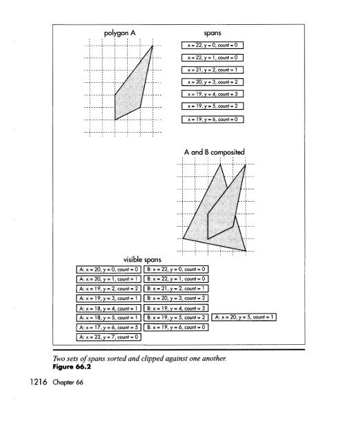
and clipping the spans against each other until only the visible portions of visible spans are left to be drawn, as shown in Figure 66.2. This may sound a lot like z-buffering (which is simply too slow for use in drawing the world, although it’s fine for smaller moving objects, as described earlier), but there are crucial differences. By contrast with z-buffering, only visible portions of visible spans are scanned out pixel by pixel (although all polygon edges must still be rasterized). Better yet, the sorting that z-buffering does at each pixel becomes a per-span operation with sorted spans, and because of the coherence implicit in a span list, each edge is sorted only against some of the spans on the same line and is clipped only to the few spans that it overlaps horizontally. Although complex scenes still take longer to process than simple scenes, the worst case isn’t as bad as with the beam tree or back-to-front approaches, because there’s no overdraw or scanning of hidden pixels, because complexity is limited to pixel resolution and because span coherence tends to limit the worst-case sorting in any one area of the screen. As a bonus, the output of sorted spans is in precisely the form that a low-level rasterizer needs, a set of span descriptors, each consisting of a start coordinate and a length. In short, the sorted spans approach meets our original criteria pretty well; although it isn’t zero-cost, it’s not horribly expensive, it completely eliminates both overdraw and pixel scanning of obscured portions of polygons and it tends to level worst-case performance. We wouldn’t want to rely on sorted spans alone as our hidden-surface mechanism, but the precalculated PVS reduces the number of polygons to a level that sorted spans can handle quite nicely. So we’ve found the approach we need; now it’s just a matter of writing some code and we’re on our way, right? Well, yes and no. Conceptually, the sorted-spans approach is simple, but it’s surprisingly difficult to implement, with a couple of major design choices to be made, a subtle mathematical element, and some tricky gotchas that I’ll have to defer until Chapter 67. Let’s look at the design choices first. Edges versus Spans The first design choice is whether to sort spans or edges (both of which fall into the general category of “sorted spans”). Although the results are the same both ways, a list of spans to be drawn, with no overdraw, the implementations and performance implications are quite different, because the sorting and clipping are performed using very different data structures. With span-sorting, spans are stored in x-sorted, linked list buckets, typically with one bucket per scan line. Each polygon in turn is rasterized into spans, as shown in Figure 66.1, and each span is sorted and clipped into the bucket for the scan line the span is on, as shown in Figure 66.2, so that at any time each bucket contains the nearest spans encountered thus far, always with no overlap. This approach involves generating all spans for each polygon in turn, with each span immediately being sorted, clipped, and added to the appropriate bucket. Quake‘s Hidden-Surface Removal 1 21 5
polygon A I I I I I I spans 1 x = 22, y = 0, count = o I I x=22,v= 1,count=0 I x=21.v=2,count=1 I I x = 20. v = 3. count = 2 I I A and B composited visible spans A: x = 20, y = 0, count = 0 B: x = 22, y = 0, count = 0 I , , , , , A:x=20,y=l,count=l Ax=19,y=2,count=2 B:x=22,y=l,count=O B:x=21,y=2,count=l Two sets of spans sorted and clipped against one another: Figure 66.2 1 21 6 Chapter 66
Page 1 and 2: chapter 66 quake's hidden-surface r
Page 3 and 4: Apart from giving me a clue as to w
Page 5: hot spots in which the frame rate b
Page 9 and 10: Active Edge List . I Current edge;
Page 11 and 12: make a few forward references to as
Page 13: sorting on l/z, we’re able to lea

quake's hidden-surface removal

You also want an ePaper? Increase the reach of your titles

Delete template?

Save as template?