6. Spatial analysis of multivariate ecological data - Laboratoire de ...
6. Spatial analysis of multivariate ecological data - Laboratoire de ...
6. Spatial analysis of multivariate ecological data - Laboratoire de ...

You also want an ePaper? Increase the reach of your titles
YUMPU automatically turns print PDFs into web optimized ePapers that Google loves.
Université Laval Analyse multivariable - mars-avril 2008 1<br />
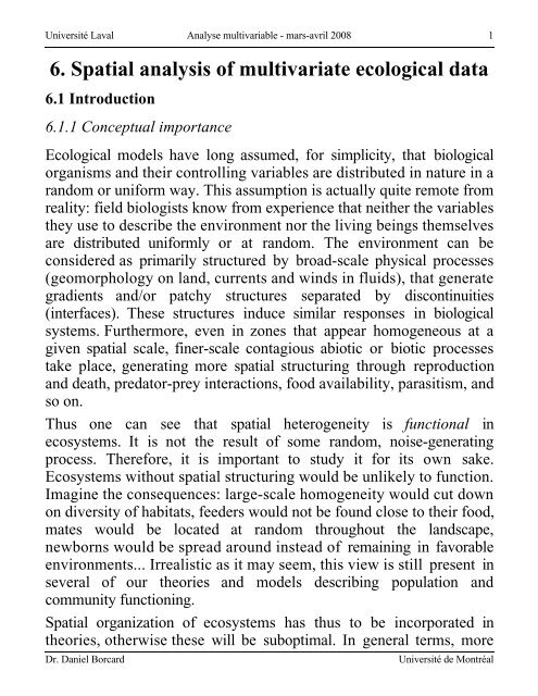
<strong>6.</strong> <strong>Spatial</strong> <strong>analysis</strong> <strong>of</strong> <strong>multivariate</strong> <strong>ecological</strong> <strong>data</strong><br />
<strong>6.</strong>1 Introduction<br />
<strong>6.</strong>1.1 Conceptual importance<br />
Ecological mo<strong>de</strong>ls have long assumed, for simplicity, that biological<br />
organisms and their controlling variables are distributed in nature in a<br />
random or uniform way. This assumption is actually quite remote from<br />
reality: field biologists know from experience that neither the variables<br />
they use to <strong>de</strong>scribe the environment nor the living beings themselves<br />
are distributed uniformly or at random. The environment can be<br />
consi<strong>de</strong>red as primarily structured by broad-scale physical processes<br />
(geomorphology on land, currents and winds in fluids), that generate<br />
gradients and/or patchy structures separated by discontinuities<br />
(interfaces). These structures induce similar responses in biological<br />
systems. Furthermore, even in zones that appear homogeneous at a<br />
given spatial scale, finer-scale contagious abiotic or biotic processes<br />
take place, generating more spatial structuring through reproduction<br />
and <strong>de</strong>ath, predator-prey interactions, food availability, parasitism, and<br />
so on.<br />
Thus one can see that spatial heterogeneity is functional in<br />
ecosystems. It is not the result <strong>of</strong> some random, noise-generating<br />
process. Therefore, it is important to study it for its own sake.<br />
Ecosystems without spatial structuring would be unlikely to function.<br />
Imagine the consequences: large-scale homogeneity would cut down<br />
on diversity <strong>of</strong> habitats, fee<strong>de</strong>rs would not be found close to their food,<br />
mates would be located at random throughout the landscape,<br />
newborns would be spread around instead <strong>of</strong> remaining in favorable<br />
environments... Irrealistic as it may seem, this view is still present in<br />
several <strong>of</strong> our theories and mo<strong>de</strong>ls <strong>de</strong>scribing population and<br />
community functioning.<br />
<strong>Spatial</strong> organization <strong>of</strong> ecosystems has thus to be incorporated in<br />
theories, otherwise these will be suboptimal. In general terms, more<br />
Dr. Daniel Borcard<br />
Université <strong>de</strong> Montréal
Université Laval Analyse multivariable - mars-avril 2008 2<br />
and more theories admit that the elements <strong>of</strong> an ecosystem that are<br />
close to one another in space or time are more likely to be influenced<br />
by the same generating processes. Such is the case, for instance, for<br />
the theories <strong>of</strong> competition, succession, evolution and adaptation<br />
(historic autocorrelation), maintenance <strong>of</strong> species diversity, parasitism,<br />
population genetics, population growth, predator-prey interactions, and<br />
social behaviour.<br />
<strong>6.</strong>1.2 Importance in sampling strategy<br />
The very fact that every living community is spatially structured has its<br />
consequences on the sampling strategies. One should be aware that<br />
the sampling strategy strongly influences the perception <strong>of</strong> the spatial<br />
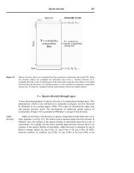
structure <strong>of</strong> the sampled population or community. For instance, in a<br />
site where the variables to be sampled are structured in more or less<br />
regular patches, systematic sampling could lead to completely altered<br />
estimations <strong>of</strong> the spatial structure if the intersample distance is larger<br />
than one half <strong>of</strong> the inter-patch distance (Figure 35, see below).<br />
This example may seem trivial especially to botanists....but botanists<br />
have a major advantage in that they see what they sample. This is not<br />
the case in, say, ecology <strong>of</strong> aquatic or soil organisms. When one<br />
samples a soil community following a systematic pattern, for example,<br />
it is quite possible that a part <strong>of</strong> the sampled species distributions will<br />
be estimated correctly, whereas some other will be totally<br />
misinterpreted. Thus, when one aims to study the spatial distribution <strong>of</strong><br />
organisms, a random-based sampling strategy seems preferable, in that<br />
it allows various and unrelated inter-sample distances to be sampled.<br />
Even when mapping is planned, it is always possible to estimate a<br />
regular grid <strong>of</strong> values on the basis <strong>of</strong> a randomly placed set <strong>of</strong><br />
measurements.<br />
Dr. Daniel Borcard<br />
Université <strong>de</strong> Montréal
Université Laval Analyse multivariable - mars-avril 2008 3<br />
Figure 35 - The danger <strong>of</strong> systematic sampling<br />
<strong>6.</strong>1.3 Importance in statistics<br />
When the variables to be sampled are spatially structured, one <strong>of</strong> the<br />
most fundamental assumptions <strong>of</strong> the classical statistics, that is, the<br />
assumption <strong>of</strong> in<strong>de</strong>pendance <strong>of</strong> the observations (or, more precisely, <strong>of</strong><br />
residuals), is violated. In a situation where no spatial structure is<br />
present, the resemblance patterns between all pairs <strong>of</strong> sample units are<br />
in<strong>de</strong>pendant <strong>of</strong> the geographical distances between the sample units. In<br />
other words, one cannot predict the value <strong>of</strong> a variable (or the species<br />
composition <strong>of</strong> a community sample unit) on the basis <strong>of</strong> a few other,<br />
neighbouring units. On the contrary, when a spatial structure exists<br />
Dr. Daniel Borcard<br />
Université <strong>de</strong> Montréal
Université Laval Analyse multivariable - mars-avril 2008 4<br />
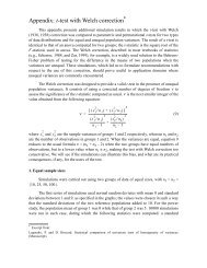
and one knows its general shape (gradient, patches...), one can predict<br />
at least roughly the content <strong>of</strong> a sample unit on the basis <strong>of</strong> the other<br />
ones on the basis <strong>of</strong> their locations. Such a sample set (or its variables)<br />
is said to be spatially autocorrelated (Figure 36).<br />
Figure 36 - Three types <strong>of</strong> spatial structures.<br />
Dr. Daniel Borcard<br />
Université <strong>de</strong> Montréal
Université Laval Analyse multivariable - mars-avril 2008 5<br />
Due to the violation <strong>of</strong> the assumption <strong>of</strong> in<strong>de</strong>pendance <strong>of</strong> the<br />
observations, it is not possible to perform standard statistical tests <strong>of</strong><br />
hypotheses on spatially autocorrelated <strong>data</strong>. In most <strong>of</strong> the natural<br />
cases, the <strong>data</strong> are positively autocorrelated at short distances, which<br />
means that any two close sample units resemble more each other than<br />
predicted by a random (uncorrelated) structure. In such cases, for<br />
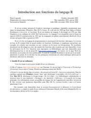
instance, the classical statistical procedures estimate a confi<strong>de</strong>nce<br />
interval around a Pearson correlation coefficient narrower than it is in<br />
reality, so that one <strong>de</strong>clares too <strong>of</strong>ten that the coefficient is different<br />
from zero (inflated type I error, Figure 37):<br />
Figure 37 - Un<strong>de</strong>restimation <strong>of</strong> the confi<strong>de</strong>nce interval around a<br />
Pearson r correlation coefficient in the presence <strong>of</strong> autocorrelation.<br />
One could un<strong>de</strong>rstand this from the point <strong>of</strong> view <strong>of</strong> the <strong>de</strong>grees <strong>of</strong><br />
freedom: normally one counts one <strong>de</strong>gree <strong>of</strong> freedom for each<br />
in<strong>de</strong>pendant observation, and this allows one to choose the appropriate<br />
statistical distribution for the given test. Now, if the observations are<br />
not in<strong>de</strong>pendant but rather autocorrelated, each new observation does<br />
not bring a full <strong>de</strong>gree <strong>of</strong> freedom, but only a fraction. It follows that<br />
the total actual number <strong>of</strong> <strong>de</strong>grees <strong>of</strong> freedom is smaller than estimated<br />
by the classical procedures. Thus the consequence: for a given total<br />
variance, the smaller the number <strong>of</strong> d.f., the broa<strong>de</strong>r the actual<br />
confi<strong>de</strong>nce interval.<br />
Dr. Daniel Borcard<br />
Université <strong>de</strong> Montréal
Université Laval Analyse multivariable - mars-avril 2008 6<br />
In limited cases there is now possible to correct for autocorrelation<br />
when estimating the number <strong>of</strong> d.f. But this is by no means an easy<br />
task.<br />
<strong>6.</strong>1.4 Importance in <strong>data</strong> interpretation and mo<strong>de</strong>lling<br />
As said previously, the spatial structuration <strong>of</strong> the living communities<br />
and their controlling environmental factors is functional. Thus, it is<br />
important to inclu<strong>de</strong> this structuration into the theories, into the <strong>data</strong><br />
analyses, and into the mo<strong>de</strong>ls.<br />
<strong>Spatial</strong> structure in the <strong>data</strong> has many consequences on the<br />
interpretation <strong>of</strong> analytical results. For instance, spatial structuration<br />
that is shared by response and explanatory variables can induce<br />
spurious correlations, leading uncorrect causal mo<strong>de</strong>ls to be accepted.<br />
Partial analyses may allow to avoid this pitfall. On the other hand,<br />
proper handling <strong>of</strong> spatial <strong>de</strong>scriptors allows to explain the <strong>data</strong><br />
variation in a more <strong>de</strong>tailed way, by disciminating between<br />
environmental, spatial, and mixed relationships.<br />
So, by taking the spatial structure into account when analyzing<br />
<strong>multivariate</strong> <strong>data</strong> sets, it is <strong>of</strong>ten possible to elucidate more <strong>ecological</strong><br />
relationships, avoid misinterpretations, and explain more <strong>data</strong> variation.<br />
This insight allows one to build more realistic mo<strong>de</strong>ls.<br />
Last but not least, spatial structures can be mapped. Mapping is not<br />
only a nice tool (or toy!) for illustration, but also a powerful way <strong>of</strong><br />
exploring <strong>data</strong> structure and generating new hypotheses, especially<br />
when the <strong>data</strong> contain a significant amount <strong>of</strong> spatial structure that is<br />
not related with the measured environmental variables.<br />
This chapter addresses the topics <strong>of</strong> some measures <strong>of</strong> autocorrelation,<br />
the components <strong>of</strong> spatial structure, and some techniques <strong>of</strong> spatial<br />
mo<strong>de</strong>ling.<br />
Dr. Daniel Borcard<br />
Université <strong>de</strong> Montréal
Université Laval Analyse multivariable - mars-avril 2008 7<br />
<strong>6.</strong> 2 The measure <strong>of</strong> spatial autocorrelation<br />
The introduction above makes clear that there are multiple reasons to<br />
test in a unambiguous way if the <strong>data</strong> are autocorrelated. One can run<br />
such tests either to verify that there is no spatial structure, and use<br />
parametric tests afterwards, or, on the contrary, to confirm the<br />
presence <strong>of</strong> a spatial structure to be able to study it in more <strong>de</strong>tail.<br />
Such tests are built on coefficients <strong>of</strong> spatial autocorrelation, that<br />
have the double advantage to test for spatial structures and provi<strong>de</strong> a<br />
simple <strong>de</strong>scription <strong>of</strong> it. Here we will first expose the tests for<br />
univariate <strong>data</strong> (Moran's I and Geary's c), and then the Mantel<br />
correlogram for <strong>multivariate</strong> <strong>data</strong>.<br />
<strong>6.</strong>2.1 One singe variable: intuitive introduction<br />
<strong>6.</strong>2.1.1 One spatial dimension<br />
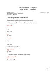
Imagine that you have collected a series <strong>of</strong> measures <strong>of</strong> bulk <strong>de</strong>nsity <strong>of</strong><br />
a soil along a transect. You can construct a graph associating the<br />
position <strong>of</strong> the sites and the measures <strong>of</strong> <strong>de</strong>nsity (Figure 38):<br />
Figure 38 - Substratum <strong>de</strong>nsity along a transect (fictitious <strong>data</strong>)<br />
Dr. Daniel Borcard<br />
Université <strong>de</strong> Montréal
Université Laval Analyse multivariable - mars-avril 2008 8<br />
In these <strong>data</strong>, one can clearly see a periodic structure. In such a case,<br />
one can predict at least approximately the value at one site on the basis<br />
<strong>of</strong> the values nearby. The series is thus autocorrelated. An easy way<br />
<strong>of</strong> studying such a series is to correlate it with itself (auto-correlating<br />
it!) several times, introducing a shift (Table XII):<br />
Table XII - Correlation <strong>of</strong> a <strong>data</strong> series with itself: auto-correlation. In<br />
this example, for <strong>de</strong>monstration purposes only, Pearson's r correlation<br />
coefficient is used for simplicity.<br />
Lag 0 : 8 9 7 5 3 1 2 1 5 6 9 9 8 5 3 1 2 1 4 6<br />
8 9 7 5 3 1 2 1 5 6 9 9 8 5 3 1 2 1 4 6 Pearson's r between the 2 series = 1<br />
Lag 1 :(8)9 7 5 3 1 2 1 5 6 9 9 8 5 3 1 2 1 4 6<br />
8 9 7 5 3 1 2 1 5 6 9 9 8 5 3 1 2 1 4(6) r = 0.75<br />
Lag 2 :(8 9)7 5 3 1 2 1 5 6 9 9 8 5 3 1 2 1 4 6<br />
8 9 7 5 3 1 2 1 5 6 9 9 8 5 3 1 2 1(4 6) r = 0.33<br />
Lag 3 :(8 9 7)5 3 1 2 1 5 6 9 9 8 5 3 1 2 1 4 6<br />
8 9 7 5 3 1 2 1 5 6 9 9 8 5 3 1 2(1 4 6) r = – 0.25<br />
Lag 4 :(8 9 7 5)3 1 2 1 5 6 9 9 8 5 3 1 2 1 4 6<br />
8 9 7 5 3 1 2 1 5 6 9 9 8 5 3 1(2 1 4 6) r = – 0.73<br />
Lag 5 :(8 9 7 5 3)1 2 1 5 6 9 9 8 5 3 1 2 1 4 6<br />
8 9 7 5 3 1 2 1 5 6 9 9 8 5 3(1 2 1 4 6) r = – 0.95<br />
Lag 6 :(8 9 7 5 3 1)2 1 5 6 9 9 8 5 3 1 2 1 4 6<br />
8 9 7 5 3 1 2 1 5 6 9 9 8 5(3 1 2 1 4 6) r = – 0.81<br />
Lag 7 :(8 9 7 5 3 1 2)1 5 6 9 9 8 5 3 1 2 1 4 6<br />
8 9 7 5 3 1 2 1 5 6 9 9 8(5 3 1 2 1 4 6) r = – 0.36<br />
Lag 8 :(8 9 7 5 3 1 2 1)5 6 9 9 8 5 3 1 2 1 4 6<br />
8 9 7 5 3 1 2 1 5 6 9 9(8 5 3 1...) r = 0.25<br />
Lag 9 :(8 9 7 5 3 1 2 1 5)6 9 9 8 5 3 1 2 1 4 6<br />
8 9 7 5 3 1 2 1 5 6 9(9 8 5 3...) r = 0.69<br />
Lag 10:(8 9 7 5 3 1 2 1 5 6)9 9 8 5 3 1 2 1 4 6<br />
8 9 7 5 3 1 2 1 5 6(9 9 8 5...) r = 0.99<br />
Lag 11:(8 9 7 5 3 1 2 1 5 6 9)9 8 5 3 1 2 1 4 6<br />
8 9 7 5 3 1 2 1 5(6 9 9 8...) r = 0.82<br />
Dr. Daniel Borcard<br />
Université <strong>de</strong> Montréal
Université Laval Analyse multivariable - mars-avril 2008 9<br />
Lag 12:(8 9 7 5 3 1 2 1 5 6 9 9)8 5 3 1 2 1 4 6<br />
8 9 7 5 3 1 2 1(5 6 9 9...) r = 0.38<br />
Lag 13:(8 9 7 5 3 1 2 1 5 6 9 9 8)5 3 1 2 1 4 6<br />
8 9 7 5 3 1 2(1 5 6 9...) r = – 0.19<br />
Lag 14:(8 9 7 5 3 1 2 1 5 6 9 9 8 5)3 1 2 1 4 6<br />
8 9 7 5 3 1(2 1 5 <strong>6.</strong>..) r = – 0.79<br />
Lag 15:(8 9 7 5 3 1 2 1 5 6 9 9 8 5 3)1 2 1 4 6<br />
8 9 7 5 3(1 2 1 5...) r = – 0.89<br />
... and we stop at lag 15, because there are not enough pairs <strong>of</strong> values<br />
left.<br />
The result <strong>of</strong> such an <strong>analysis</strong> is generally presented in the form <strong>of</strong> a<br />
correlogram, where the abscissa represents the lag, and the ordinate<br />
are the correlation values (Figure 39):<br />
Corrélation<br />
1<br />
0.8<br />
0.6<br />
0.4<br />
0.2<br />
0<br />
-0.2 0 1 2 3 4 5 6 7 8 9 10 11 12 13 14 15<br />
-0.4<br />
-0.6<br />
-0.8<br />
-1<br />
Pas (décalage <strong>de</strong> la série p.r. à elle-même)<br />
Figure 39 - Correlogram <strong>of</strong> the fictitious <strong>data</strong> <strong>of</strong> Fig. 38. Beware: the<br />
lag ("pas") does not represent spatial coordinates, but reciprocal<br />
distances among sites! For instance, at lag 5, the r = –0.95 means that<br />
any pair <strong>of</strong> sites whose members are 5 units apart (for instance sites 3<br />
and 8, or 10 and 15...) probably have very different values <strong>of</strong> <strong>de</strong>nsity:<br />
one <strong>of</strong> the sites has a high value, the other a low one.<br />
Dr. Daniel Borcard<br />
Université <strong>de</strong> Montréal
Université Laval Analyse multivariable - mars-avril 2008 10<br />
<strong>6.</strong>2.1.2 Two spatial dimensions (surface)<br />
The next step <strong>of</strong> our reasoning is to extend it to a surface, in the case<br />
<strong>of</strong> an isotropic process (the spatial pattern is more or less i<strong>de</strong>ntical in<br />
all directions). In this case, one can no more organize the <strong>data</strong> in a<br />
linear series. Rather, one computes a matrix <strong>of</strong> Eucli<strong>de</strong>an<br />
(geographical) distances among all pairs <strong>of</strong> sites, and then the distances<br />
are grouped in classes. For instance, all distances shorter than 1 meter<br />
belong to class 1, the distances between 1 and 2 meters are put in<br />
class 2, and so on. Table XIII gives an example:<br />
Table XIII - Construction <strong>of</strong> a matrix <strong>of</strong> classes <strong>of</strong> distance<br />
2 3 4 5 6 2 3 4 5 6<br />
1 0.23 2.82 1.65 0.89 1.23 1 3 2 1 2<br />
2 1.45 2.44 0.32 1.87 2 3 1 2<br />
3 3.56 0.09 2.11 -> 4 1 3<br />
4 2.70 1.15 3 2<br />
5 1.34 2<br />
Matrix <strong>of</strong> Eucli<strong>de</strong>an distances Matrix <strong>of</strong> distance classes<br />
On this basis (but with more than 6 sites!) one could compute<br />
autocorrelation indices for the 4 classes <strong>of</strong> geographical distances. For<br />
instance, for class 1 the value would be computed on the basis <strong>of</strong> pairs<br />
1-2, 1-5, 2-5 and 3-5. And so on. For n objects, one always has n(n–<br />
1)/2 distances, that should be grouped into an appropriate number <strong>of</strong><br />
classes: neither too high (too few values in each class) nor too low (to<br />
avoid the <strong>analysis</strong> to be too coarse). Sturge's rule is <strong>of</strong>ten used to<br />
<strong>de</strong>ci<strong>de</strong> how many classes are appropriate:<br />
Nb <strong>of</strong> classes = 1 + 3.3 log 10 (m)<br />
(roun<strong>de</strong>d to the nearest integer)<br />
where m is, in this case, the number <strong>of</strong> distances in the upper<br />
triangular matrix <strong>of</strong> distances (excluding the diagonal).<br />
Dr. Daniel Borcard<br />
Université <strong>de</strong> Montréal
Université Laval Analyse multivariable - mars-avril 2008 11<br />
<strong>6.</strong>2.2 Indices <strong>of</strong> spatial autocorrelation: Moran's I and Geary's c<br />
In practice, the two mostly used indices are Moran's I, which behaves<br />
approximately like a Pearson correlation coefficient, and Geary's c,<br />
which is a sort <strong>of</strong> distance.<br />
Moran's I is computed as follows (for distance class d):<br />
I(d) =<br />
1<br />
W<br />
n<br />
∑<br />
n<br />
h=1i=1<br />
and Geary's c:<br />
c(d) =<br />
n<br />
( )( y i − y )<br />
∑w hi y h − y<br />
1<br />
n<br />
n<br />
1<br />
∑ ∑<br />
2W h=1<br />
1<br />
( n −1)<br />
n<br />
∑( y i − y ) 2<br />
i=1<br />
i=1<br />
n<br />
w hi ( y h − y i ) 2<br />
∑( y i − y ) 2<br />
i=1<br />
for h ≠ i<br />
for h ≠ i<br />
y h and y i are the values <strong>of</strong> the variable in objects h and i; n is the<br />
number <strong>of</strong> objects; the weights w are equal to 1 when pair (h,i)<br />
belongs to distance class d (the one for which the in<strong>de</strong>x is computed)<br />
and 0 otherwise. W is the sum <strong>of</strong> all w hi , i.e. the number <strong>of</strong> pairs <strong>of</strong><br />
objects belonging to distance class d.<br />
Moran's I generally varies between –1 and +1, although values<br />
beyond these limits are not impossible. Positive autocorrelation yields<br />
positive values <strong>of</strong> I, and negative autocorrelation produces negative<br />
values. Moran's I expected value in the absence <strong>of</strong> autocorrelation is<br />
equal to E(I) = – (n – 1) -1 i.e., close to 0 when n is large.<br />
Geary's c varies from 0 to some unspecified value larger than 1.<br />
Positive autocorrelation translates into values from 0 to 1, while<br />
negative autocorrelation yields values larger than 1. Geary's c<br />
expectation in the absence <strong>of</strong> autocorrelation is equal to E(c) = 1.<br />
Dr. Daniel Borcard<br />
Université <strong>de</strong> Montréal
Université Laval Analyse multivariable - mars-avril 2008 12<br />
Example<br />
The 8 x 8 grid below (Table XIV and Figure 40) is a fictitious <strong>data</strong> set<br />
where the value <strong>of</strong> a variable z has been measured on a regular<br />
sampling <strong>de</strong>sign. One can see a gradient in the <strong>data</strong>.<br />
Table XIV - Fictitious, spatially referenced sample set. 64 sites.<br />
11 10 9 7 7 6 4 2<br />
9 11 7 6 5 3 2 2<br />
10 9 6 10 8 4 5 3<br />
8 9 7 5 4 3 3 2<br />
7 6 5 6 4 4 3 2<br />
5 5 5 4 5 3 1 3<br />
5 4 3 2 3 3 2 2<br />
3 4 2 2 1 3 1 1<br />
Figure 40 - Grid map <strong>of</strong> the <strong>data</strong> given in Table IX.<br />
Each site is characterized by its x - y spatial coordinates and the value<br />
<strong>of</strong> the measured variable, z. In this example, let us state that the<br />
horizontal and vertical intersite distance is equal to 1 m. The<br />
computation <strong>of</strong> a correlogram involves 4 steps:<br />
Dr. Daniel Borcard<br />
Université <strong>de</strong> Montréal
Université Laval Analyse multivariable - mars-avril 2008 13<br />
1. Computation <strong>of</strong> a matrix <strong>of</strong> Eucli<strong>de</strong>an distances among sites.<br />
2. Transformation <strong>of</strong> these distances into classes <strong>of</strong> distances.<br />
3. Computation <strong>of</strong> Moran's I or Geary's c for all distance classes.<br />
4. Drawing <strong>of</strong> the correlograms.<br />
The hypotheses <strong>of</strong> the tests run on each distance class can be wor<strong>de</strong>d<br />
as follows:<br />
H 0 : there is no spatial autocorrelation. The values <strong>of</strong> variable z are<br />
spatially in<strong>de</strong>pen<strong>de</strong>nt. Each Moran's I or Geary's c value is close<br />
to its expectation.<br />
H 1 : there is significant spatial autocorrelation in the <strong>data</strong>. At least one<br />
autocorrelation value is significant at the Bonferroni-corrected<br />
level <strong>of</strong> significance (see below).<br />
The result below (with 6 equidistant classes) has been obtained using<br />
the R package for <strong>multivariate</strong> <strong>data</strong> <strong>analysis</strong> by Pierre Legendre,<br />
Philippe Casgrain and Alain Vaudor. This package, not to be confused<br />
with the R language, is available for Macintosh (Classic environment)<br />
from Pierre Legendre's web site:<br />
http://www.bio.umontreal.ca/legendre/<br />
Classes équidistantes<br />
Classe Limite sup. Fréq.<br />
1 1.64992 210<br />
2 3.29983 556<br />
3 4.94975 442<br />
4 <strong>6.</strong>59967 560<br />
5 8.24958 218<br />
6 9.89950 30<br />
Dr. Daniel Borcard<br />
Université <strong>de</strong> Montréal
Université Laval Analyse multivariable - mars-avril 2008 14<br />
FICHIER DE DONNEES grad.8x8.r<br />
Option du mouvement: Matrice SIMIL<br />
Note: les probabilités sont plus significatives près <strong>de</strong> zéro<br />
les probabilités sont à plus ou moins; 0.00100<br />
H0: I = 0 I = 0 C = 1 C = 1<br />
H1: I > 0 I < 0 C < 1 C > 1<br />
Dist.,I(Moran), p(H0), p(H0), C(Geary), p(H0), p(H0), Card.*<br />
1 0.6723 0.000 0.2366 0.000 420<br />
2 0.3995 0.000 0.4601 0.000 1112<br />
3 0.0225 0.177 0.8660 0.008 884<br />
4 -0.3678 0.000 1.4245 0.000 1120<br />
5 -0.7674 0.000 2.0580 0.000 436<br />
6 -1.0667 0.000 2.7131 0.000 60<br />
Total 4032<br />
* Card. means "cardinality", i.e. the number <strong>of</strong> pairs <strong>of</strong> observations in each distance class, in a square<br />
distance matrix, diagonal exclu<strong>de</strong>d.<br />
The following correlograms can be drawn from the results above:<br />
Figure 41 - Moran's I correlogram, <strong>data</strong> from Table XIV.<br />
Dr. Daniel Borcard<br />
Université <strong>de</strong> Montréal
Université Laval Analyse multivariable - mars-avril 2008 15<br />
Figure 42 - Geary's c correlogram, <strong>data</strong> from Table XIV.<br />
In these graphs, the black squares are significant values (at an<br />
uncorrected α level <strong>of</strong> 0.05, but see below!) and white squares non<br />
significant ones. The output file gives the exact probabilities.<br />
The opposite aspect <strong>of</strong> the curves illustrates well the fact that Moran's<br />
I behaves like a correlation (positive values mean positive<br />
autocorrelation) while Geary's c behaves like a distance (lowest value<br />
for highest positive autocorrelation).<br />
<strong>6.</strong>2.3 Correction for multiple testing<br />
One problem remains, related to the α probability level <strong>of</strong> rejection <strong>of</strong><br />
the null hypothesis. Such a threshold is <strong>de</strong>fined for one test. In our<br />
case, since we computed six autocorrelation values (one for each<br />
distance class), six tests have been performed simultaneously. In such<br />
Dr. Daniel Borcard<br />
Université <strong>de</strong> Montréal
Université Laval Analyse multivariable - mars-avril 2008 16<br />
a case, the type I error (rejecting H 0 when it is true) is no more 0.05 (if<br />
this was the selected level). For one test, a threshold <strong>of</strong> 5% means that,<br />
on average, among 100 tests run on completely random variables, 5<br />
will (wrongly) reject H 0 and 95 will not. Cumulating 6 tests at the 5%<br />
level means that the chances <strong>of</strong> rejecting H 0 at least once is equal to 1<br />
– 0.95 6 = 0.265 instead <strong>of</strong> 0.05 ! The most drastic (conservative)<br />
remedy to this situation is called the Bonferroni correction, which<br />
consists in dividing the global threshold level by the number <strong>of</strong><br />
simultaneous tests. In our case, for each correlogram, this means that,<br />
globally, the correlogram will be <strong>de</strong>clared significant if at least one<br />
autocorrelation value is significant at the corrected α level <strong>of</strong> 0.05/6 =<br />
0.0083. One can verify that, with this correction, the global chances <strong>of</strong><br />
accepting H 0 when it is true is equal to (1 – 0.0083) 6 ≈ 0.95.<br />
This correction is very conservative, however, and can lead to type II<br />
error (accepting H 0 when it is false) when the tests involved in the<br />
multiple comparison are not in<strong>de</strong>pen<strong>de</strong>nt, i.e. when they address a<br />
series <strong>of</strong> related questions and <strong>data</strong>. Several alternatives have been<br />
proposed in the literature. An interesting one is the Holm correction.<br />
It consists in (1) running all the k tests, ( 2) or<strong>de</strong>ring the probabilities in<br />
increasing or<strong>de</strong>r, and (3) correcting each α significance level by<br />
dividing it by (1 + the number <strong>of</strong> remaining tests) in the or<strong>de</strong>red series.<br />
In this way, the first level is divi<strong>de</strong>d by k, the second one by k – 1, and<br />
so on. The procedure stops when a non-significant value is<br />
encountered.<br />
<strong>6.</strong>2.4 Multidimensional <strong>data</strong>: the Mantel correlogram<br />
If one wants to explore the autocorrelation structure <strong>of</strong> a <strong>multivariate</strong><br />
<strong>data</strong> set (for instance a matrix <strong>of</strong> species abundances), on can resort to<br />
the Mantel correlogram. This technique is based on the Mantel<br />
statistic. Each class <strong>of</strong> the matrix <strong>of</strong> distance classes is represented by a<br />
binary (0 - 1) matrix where the pairs <strong>of</strong> objects belonging to that class<br />
receive the value 1 and the others 0. The tests are permutational (as in<br />
Dr. Daniel Borcard<br />
Université <strong>de</strong> Montréal
Université Laval Analyse multivariable - mars-avril 2008 17<br />
the case <strong>of</strong> the Mantel test). If the standardized Mantel statistic is used,<br />
the values are ranged between -1 and +1 and the interpretation <strong>of</strong> the<br />
Mantel correlogram is similar to that <strong>of</strong> the Moran correlogram,<br />
bearing in mind that the expectation <strong>of</strong> the Mantel statistic un<strong>de</strong>r H 0 is<br />
strictly 0.<br />
<strong>6.</strong>2.5 Remarks<br />
1. Many other structure functions are available to <strong>de</strong>scribe and mo<strong>de</strong>l<br />
spatial structures. A very important one is the semi-variogram, which<br />
uses a measure <strong>of</strong> variance among values <strong>of</strong> sites belonging to various<br />
distance classes to build a mo<strong>de</strong>l that can be used either to <strong>de</strong>scribe the<br />
spatial structure (as in the case <strong>of</strong> the correlogram) or to mo<strong>de</strong>l it,<br />
especially for mapping and prediction purposes (as in the case <strong>of</strong><br />
kriging).<br />
2. Unless otherwise specified, these methods consi<strong>de</strong>r that the spatial<br />
structures are isotropic (same in all directions). But anisotropy can be<br />
addressed in several ways, for instance by modifying the matrix <strong>of</strong><br />
distance classes.<br />
3. When statistical tests are run to i<strong>de</strong>ntify spatial structures, they<br />
require that the condition <strong>of</strong> second-or<strong>de</strong>r stationarity be satisfied.<br />
This condition states that the expected value (mean) and spatial<br />
covariance (numerator <strong>of</strong> Moran's I) <strong>of</strong> the variable are the same all<br />
over the study area, and the variance (<strong>de</strong>nominator) is finite. A relaxed<br />
form <strong>of</strong> stationarity hypothesis, the intrinsic assumption, states that<br />
the differences (y h – y i ) for any distance must have zero mean and<br />
constant and finite variance over the study area.<br />
Dr. Daniel Borcard<br />
Université <strong>de</strong> Montréal