Introduction to Soft Matter Simulations - ESPResSo
Introduction to Soft Matter Simulations - ESPResSo
Introduction to Soft Matter Simulations - ESPResSo

Create successful ePaper yourself
Turn your PDF publications into a flip-book with our unique Google optimized e-Paper software.
Simulating <strong>Soft</strong> <strong>Matter</strong> with<br />
<strong>ESPResSo</strong>, <strong>ESPResSo</strong>++ and<br />
VOTCA!<br />
Christian Holm!<br />
Institut für Computerphysik, Universität Stuttgart<br />
Stuttgart, Germany!<br />
1!
Intro <strong>to</strong> <strong>Soft</strong> <strong>Matter</strong> <strong>Simulations</strong>!<br />
• What is <strong>Soft</strong> <strong>Matter</strong>?<br />
• What can simulations do for you?<br />
• What is needed <strong>to</strong> perform good simulations?<br />
• Bits and pieces of necessary background<br />
information for understanding molecular<br />
simulations<br />
• <strong>ESPResSo</strong>: his<strong>to</strong>ry, aim, background
What is <strong>Soft</strong> <strong>Matter</strong>?
What is <strong>Soft</strong> <strong>Matter</strong>?<br />
….and why is it interesting?!
What is <strong>Soft</strong> <strong>Matter</strong>?
What is <strong>Soft</strong> <strong>Matter</strong>?<br />
• Gummy bears, gels, networks: Rubber, low fat food,<br />
• Fibers (z.B. Goretex, Nylon)…<br />
• Colloidal systems: milk, mayonnaise, paints,<br />
cosmetics…<br />
•“Simple” plastics: joghurt cups, many car parts, CDs, …<br />
• Membranes: cell walls, artificial tissue, vesicles…<br />
• Many parts of the cell, cy<strong>to</strong>skele<strong>to</strong>n, nucleus<br />
• Most biomolecules (RNA, DNA, proteins, amino-acids)<br />
• Liquid crystals<br />
• Many applications: smart materials (actua<strong>to</strong>rs, sensors,<br />
pho<strong>to</strong>nic crystals), biotechnology, biomedicin<br />
(hyperthermia, drug targeting, cell separation<br />
techniques), model systems for statistical physics
Length Scales of <strong>Soft</strong> <strong>Matter</strong>!<br />
1 fm 1pm 1 Å 1nm 10 µm 1mm 1m 1km 10 3 km 10 6 parsec<br />
<strong>Soft</strong><br />
<strong>Matter</strong><br />
10 -15 m 10 -12 m 10 -9 m 10 -6 m 10 -3 m 10 0 m 10 3 m 10 6 m<br />
7!
Length Scales of <strong>Soft</strong> <strong>Matter</strong>!<br />
1 Å 1nm 10 µm 1mm<br />
<strong>Soft</strong><br />
<strong>Matter</strong><br />
10 -15 m 10 -12 m 10 -9 m 10 -6 m 10 -3 m 10 0 m 10 3 m 10 6 m<br />
1 nm 10 nm 100 nm 1 µm 10 µm 100 µm<br />
8!<br />
CH 4<br />
Magnetische<br />
NP
Who needs <strong>Simulations</strong>?!<br />
<br />
<br />
<br />
<br />
<br />
<br />
Goal: Understanding and prediction of interesting systems!<br />
Computer science: Network simulations, “emulations” of not-yetexisting<br />
CPUs, …!<br />
Economy: <strong>Simulations</strong> of economical cycles!<br />
Biology: <strong>Simulations</strong> of metabolic networks, ecological simulations<br />
(e.g. Preda<strong>to</strong>r-prey-systems, population dynamics)!<br />
Physics: <strong>Simulations</strong> of quantum systems, simulations of mechanical<br />
systems, astronomical simulations, weather prediction!<br />
Here: Physics/Chemistry/Boplogy: Simulation of <strong>Soft</strong> <strong>Matter</strong> and Bio<br />
Systems (Polymers, Fluids, Proteins, …)!
The New Trinity of Physics!<br />
Experiment!<br />
Theory<br />
Computer simulations<br />
( Computer experiments)<br />
Why using simulations in physics?!<br />
<br />
<br />
<br />
<br />
All laws of nature can be expressed as mathematical formulas!<br />
However, only few physical systems can be solved analytically!<br />
<strong>Simulations</strong> can be used <strong>to</strong> numerically solve the most complex<br />
formulas and <strong>to</strong> compare them <strong>to</strong> experimental results !<br />
System properties can be estimated without actually creating the<br />
system (cheaper, simpler, faster and/or less dangerous, well<br />
controlled)!
Natural Speed-ups and ....!<br />
Computer power doubles every 24 months ends<br />
Future: computer power / 1000 Euro ?<br />
Need <strong>to</strong> exploit parallelism!
other architectures (GPUs) and...!<br />
http://developer.nvidia.com/cuda/nvidia-gpucomputing-documentation
... more clever Algorithms can help!!<br />
Smart Algorithms can (and do) outperforme Moore‘s law !!
Molecular <strong>Simulations</strong> !<br />
<br />
<br />
<br />
In a molecular simulation, the evolution of the states of a<br />
molecular system needs <strong>to</strong> be simulated!<br />
In principle, only a pure quantum mechanical description of<br />
such a system is exact (careful, even here are pitfalls! How<br />
many exact solutions are known?)!<br />
<br />
<br />
<br />
Only very small systems can be simulated on that<br />
level !<br />
The system has <strong>to</strong> be simplified (“coarse-grained”)!<br />
First step: Classical A<strong>to</strong>ms and Interactions!<br />
Real systems have ~10 23 a<strong>to</strong>ms!<br />
<br />
<br />
<br />
A statistical description is needed!<br />
Only a part of a molecular system can be simulated!<br />
The simulated system has significant boundaries!
Coarse-graining!<br />
<br />
<br />
<br />
<br />
<br />
A model consists of a number of<br />
Degrees of Freedom (e.g. the<br />
a<strong>to</strong>m positions) and the<br />
Interactions between them!<br />
Coarse-graining:!<br />
<br />
<br />
reduce the number of degrees of<br />
freedom by keeping only the<br />
“important” degrees of freedom!<br />
Use “effective” interactions!<br />
Classical first step: A<strong>to</strong>ms and<br />
Interactions (all-a<strong>to</strong>m or a<strong>to</strong>mistic)!<br />
Further coarse-graining is often<br />
needed and useful!<br />
For <strong>Soft</strong> <strong>Matter</strong> we are often on<br />
the molecular and mesoscopic<br />
level!<br />
All-a<strong>to</strong>m<br />
Quantum<br />
Mesoscopic<br />
Fluid Methods<br />
Molecular<br />
Continuum
Computational Approaches!<br />
• Quantum: ab-initio QM or first principles high-level<br />
QM, PHF, MP2,Car-Parrinello MD, Born-Oppenheimer<br />
MD, TBDFT, hybrid embedded QM/MM, ...!<br />
• A<strong>to</strong>mistic: Classical Force Field AA MD,MC!<br />
• Coarse-grained: Classical DFT, Molecular Dynamics,<br />
Monte Carlo, Field theoretic methods (SCFT)!<br />
• Mesoscopic Fluid: Lattice-Boltzmann, MPC, DPD!<br />
• Continuum Solvers: Computational Fluid Dynamics<br />
codes (Navier-S<strong>to</strong>kes), Poisson-Boltzmann, Lattice-<br />
Boltzmann, FEM!
Available Programs:!<br />
• First principles Quantum: TURBOMOLE, Molpro (Stuttgart),<br />
Gaussian,...<br />
• DFT: CP2K, Car-Parrinello MD, Quantum Espresso,<br />
Wien2K,... Look on www.psi-k.org<br />
• All-A<strong>to</strong>m: GROMOS, GROMACS, NAMD, AMBER, CHARM,<br />
DL_POLY, LAMMPS...<br />
• Coarse-grained: DL_POLY, LAMMPS, <strong>ESPResSo</strong>, OCTA,...<br />
Continuum<br />
• For PB: Delphi, APBS,UHBD<br />
• For FEM: DUNE, more on http://www.cfd-online.com/Wiki/<br />
Codes<br />
• Lattice-Boltzmann: openLB<br />
• .......much more than I can list
Making Molecular <strong>Simulations</strong>!<br />
How <strong>to</strong> make a molecular simulation?!<br />
Choose the system <strong>to</strong> be simulated !<br />
<br />
<br />
<br />
<br />
<br />
Choose the model and coarse-graining level of the<br />
simulation !<br />
Determine the initial state of the model!<br />
Simulate the model (using an appropriate algorithm<br />
and appropriate <strong>to</strong>ols)!<br />
Analyze and interpret the results!<br />
Executing the simulation is only a small part of the<br />
work!!
Possible errors!<br />
<strong>Simulations</strong> have plenty of sources for errors!!<br />
<br />
<br />
<br />
<br />
<br />
Errors of the boundary of the system!<br />
Errors of the initial state!<br />
Errors of the model / level of coarse-graining!<br />
Numerical errors (Errors of the simulation)!<br />
Errors of the interpretation / analysis!<br />
Theory and experimental<br />
verifications are still needed<br />
Remember Murphy‘s Law!
What do I need <strong>to</strong> know...!<br />
...before I start simulating? !<br />
• Statistical Mechanics!<br />
• Theory behind my system (i.e. <strong>Soft</strong><br />
<strong>Matter</strong> theory)!<br />
• The program I am using (best way is <strong>to</strong><br />
write it yourself!)!<br />
• Background of the algorithm (strength,<br />
weakness, limitations)!<br />
• Clever ways of analyzing the data!
Aim of this week long tu<strong>to</strong>rial?!<br />
• Describe some Algorithms:!<br />
• Long range interactions!<br />
• CG Hydrodynamics!<br />
• Membrane simulations (Mb<strong>to</strong>ols)!<br />
• VOTCA, AdResS, <strong>ESPResSo</strong>++!<br />
• Some sample applications!<br />
• ...there is much more you need <strong>to</strong> know....!<br />
• Bits and pieces!<br />
• Meet developers for specific questions!
Periodic Boundary Conditions!<br />
<br />
<br />
<br />
<br />
<br />
<br />
<br />
<br />
Simulated systems are much smaller than “real” systems<br />
Boundaries make up a significant part of the<br />
system!<br />
Surface/Volume not small (i.e. for N=1000 the<br />
boundary makes up 49%)<br />
Trick: Periodic boundary conditions!<br />
The simulated system has infinitely many<br />
copies of itself in all directions!<br />
A particle at the right boundary interacts with<br />
the particle at the left boundary in the image!<br />
Minimum image convention: Each particle<br />
only interacts with the closest image of<br />
another particle (i.e. interaction range L/2)!<br />
Pseudo-infinite system without boundaries!<br />
Significantly reduces boundary-related errors!<br />
More tricky for long range interactions…!
Example: Modeling Liquid Argon!<br />
<br />
<br />
Very simple system:!<br />
<br />
Noble gas: no bonds<br />
between a<strong>to</strong>ms!<br />
Semi-empirical <br />
Lennard-Jones-Potential:!<br />
Closed shell: almost<br />
spherical!<br />
<br />
Contributions <strong>to</strong> the<br />
interaction (from QM):!<br />
Pauli exclusion principle:<br />
strongly repulsive core<br />
(exact functional form<br />
does not matter)!<br />
Van-der-Waals<br />
interaction: attractive<br />
interaction for larger<br />
distances ~-1/r 6!<br />
Liquid argon: σ = 3.4 Å, ε = 100 cm -1 !
All-A<strong>to</strong>m Models!<br />
<br />
<br />
Most commonly used model!<br />
Each a<strong>to</strong>m is represented by one<br />
spherical particle!<br />
A force field (FF) describes the interactions <br />
between the a<strong>to</strong>ms and consists of !<br />
a set of equations !<br />
<br />
a long table of parameters for all a<strong>to</strong>m type pairs!<br />
For different applications, various different force <br />
fields exist (e.g. GROMOS, AMBER, OPLS,<br />
Charm… )!<br />
<br />
The interactions can be split in<strong>to</strong> two groups:!<br />
<br />
<br />
Non-bonded potentials: e.g. Lennard-Jones, Coulomb!<br />
Bonded potentials for bonded a<strong>to</strong>ms!
Non-bonded Potentials!<br />
<br />
<br />
Non-bonded potentials model the interaction between a<strong>to</strong>ms<br />
that do not have bonds!<br />
Lennard-Jones potential accounts for Pauli exclusion and vander-Waals<br />
interaction:<br />
<br />
Coulomb interaction for charged a<strong>to</strong>ms:<br />
<br />
<br />
Beware: The Coloumb interaction is long-ranged. This may<br />
require special measures <strong>to</strong> compute it!!<br />
In some force fields, usually uncharged a<strong>to</strong>ms can carry<br />
partial charges <strong>to</strong> account for polarization effects in certain<br />
compounds (for example water)!
Bonded Potentials!<br />
<br />
Bonded potentials model the bonds between a<strong>to</strong>ms!<br />
Bond-stretching: harmonic 2-body potential <br />
models bond length:<br />
<br />
Classical spring potential!!<br />
Bond-angle potential (3-body) models <br />
bond angle:<br />
or!
Dihedral Potentials (4-body)!<br />
<br />
<br />
The dihedral angle is the angle between<br />
the planes of 4 bonded a<strong>to</strong>ms!<br />
Improper dihedrals keep planar groups<br />
planar (e.g. aromatic rings):<br />
<br />
<br />
again: harmonic potential!<br />
Proper dihedrals model cis/trans<br />
conformations:<br />
ξ"
How <strong>to</strong> find the FF parameters?!<br />
• Fit experimental data (density, g(r), diffusion, heat<br />
of vaporization, ...)!<br />
• use QM calculations <strong>to</strong> calculate some interaction<br />
parameters!<br />
• FF work for the situation where they were<br />
parametrized, hope carries us along...<br />
(transferability)!<br />
• Combining FF parameters is non-trivial, often<br />
needs reparametrization!
Pros and Cons of FF!<br />
• PRO:!<br />
• Fast and easy <strong>to</strong> use (practically linear scaling)!<br />
• Visualization of microscopic behavior!<br />
• Mechanistic insight!<br />
• CON:!<br />
• Quality difficult <strong>to</strong> asses!<br />
• Chemical reactions difficult <strong>to</strong> model!<br />
• Orbital interactions (polarizability) often not included!
Coarse-grained Models!<br />
<br />
<br />
<br />
<br />
<br />
Large and complex molecules (e.g.<br />
long polymers) can not be<br />
simulated on the all-a<strong>to</strong>m level!<br />
Requires coarse-graining of the<br />
model!<br />
Coarse-grained models are usually<br />
also particles (beads) and<br />
interactions (springs, …)!<br />
A bead represents a group of<br />
a<strong>to</strong>ms!<br />
Coarse-graining a molecule is<br />
highly non-trivial, see systematic<br />
coarse-graining, VOTCA, AdResS!
Gaussian Polymer in a Θ-solvent!<br />
Conformational properties of a Gaussian polymer in a <br />
Θ-solvent are that of a random walk!<br />
<br />
<br />
Basis for bead-spring model of a polymer!!<br />
Use a harmonic potential for the bonds:<br />
<br />
We can compute the partition function exactly<br />
<br />
Random walk and bead-spring model generate the<br />
same partition function!!
Gaussian Chains in Good Solvent!<br />
<br />
<br />
Θ-solvent is a special case!!<br />
Solvents are good or poor w.r. <strong>to</strong> the polymer!<br />
Good solvent can be modeled via a repulsive <br />
potential!<br />
Use the repulsive part of Lennard-Jones <br />
(aka Weeks-Chandler-Anderson)<br />
Lennard-Jones<br />
WCA<br />
<br />
FENE (Finite Extensible Nonlinear Elastic) bond<br />
FENE<br />
Harmonic<br />
<br />
Has a maximal extension/compression!<br />
Very similar <strong>to</strong> harmonic potential at r 0!
Gaussian Chains in Poor Solvent!<br />
<br />
Poor solvent can be modeled via a full!<br />
!Lennar-Jones potential!<br />
Polymer monomers experience an attraction, !<br />
<br />
<br />
!since they want <strong>to</strong> minimize contact with solvent!<br />
the quality of the solvent can be changed by!<br />
varying the attraction via the interaction parameter ε and the cut-off!<br />
Scaling laws R ∝ N ν with Flory exponent ν"<br />
RW ν = 0.5!<br />
SAW ν = 0.588 (3/5)!<br />
Globule ν<br />
€<br />
= 1/3!<br />
Rod ν = 1<br />
Lennard-Jones<br />
WCA
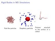
34!<br />
Charged Polymers!
Molecular Dynamics!
New<strong>to</strong>n's Equations of Motion!<br />
Basic idea of Molecular Dynamics (MD): !<br />
<br />
<br />
The system consists of point particles and interactions (e.g. a<strong>to</strong>ms and<br />
their interactions)!<br />
Solve the classical equations of motion for the particles on the computer:<br />
<br />
Can be applied <strong>to</strong> a wide range of problems:!<br />
<br />
<br />
<br />
<br />
<br />
Molecular systems (gases, fluids, polymers, proteins, liquid crystals,<br />
…)!<br />
Granular materials (sand, sugar, salt, …)!<br />
Planetary motion!<br />
Nuclear missiles!<br />
…!
Euler's Method of Integration!<br />
<br />
<br />
Numerical integration: discretize in time, time-step!<br />
Use finite differences:<br />
Taylor expand <br />
2!
Euler's Method of Integration!<br />
<br />
<br />
Numerical integration: discretize in time, time-step!<br />
Use finite differences:<br />
Taylor expand !<br />
<br />
<br />
<br />
Truncate at higher order terms!!<br />
Positions in the next time-step can be computed!!<br />
Simplest integration method, least accurate!<br />
2!
Estimating the Time-step!<br />
How large should the time-step<br />
<br />
<br />
<br />
be?!<br />
It should not cause numerical instabilities of the<br />
integration algorithm!<br />
It should allow <strong>to</strong> observe the collision of two<br />
particles!<br />
Rule of thumb: Particles should move maximally<br />
~1/10 of the particle diameter d per time-step!<br />
<br />
Time-step depends on the maximal velocity v max!
Required Iterations!<br />
A<strong>to</strong>ms /<br />
Molecules<br />
Granular<br />
matter<br />
Astrophysics<br />
Diameter d 10 -10 m 10 -3 m 10 7 m<br />
Maximal velocity 10 m/s 1 m/s 10 8 m/s<br />
v max<br />
Time-step Δt 10 -12 s 10 -4 s 10 -2 s<br />
Wanted simulation<br />
time<br />
1s 10 2 s 10 13 s<br />
Required Iterations 10 12 10 6 10 15
Good Integration Algorithms!<br />
What is a good integration algorithm?!<br />
Easy <strong>to</strong> implement, fast <strong>to</strong> compute!<br />
Numerically stable for large time-steps<br />
<strong>to</strong> allow for long simulations!<br />
Trajec<strong>to</strong>ry should be reproducible!<br />
Should conserve energy, linear and<br />
angular momentum !
Short-time Stability!<br />
<br />
<br />
<br />
Depending on the problem at<br />
hand, different properties of the<br />
integration algorithm are<br />
important!<br />
For some systems, it is important<br />
that the algorithm has a minimal<br />
error in the trajec<strong>to</strong>ry (“short-time<br />
stable”) (e.g. satellite orbits)!<br />
Note that the error in the<br />
trajec<strong>to</strong>ry always grows<br />
exponentially over time due <strong>to</strong><br />
positive Lyapunov exponents!
Long-time Stability!<br />
<br />
<br />
In molecular simulations, we want <strong>to</strong> compute statistical<br />
averages (i.e. ensemble averages) of observables!<br />
MD uses the Ergodic hypothesis:<br />
<br />
<br />
trajec<strong>to</strong>ry<br />
= ensemble!<br />
Accurate trajec<strong>to</strong>ries are not important!<br />
Instead, the correct physical ensemble should be<br />
described throughout the simulation:!<br />
<br />
<br />
<br />
Conservation of energy, linear and angular<br />
momentum!<br />
Time-reversibility!<br />
(In fact: conservation of phase space)!<br />
Integra<strong>to</strong>rs that do this are “long-time stable” <br />
(or “symplectic”)!
Verlet Algorithm!<br />
<br />
<br />
Verlet Integra<strong>to</strong>r (1967) is more accurate than Euler's<br />
method, and it is long-time stable(!)!<br />
To derive it, Taylor expand x(t) forward and backward in<br />
time<br />
<br />
This results in<br />
<br />
Straightforward algorithm, long-time stable!<br />
Bootstrapping problem: Requires for the initial<br />
step!
Velocity Verlet Algorithm!<br />
<br />
<br />
Mathematically equivalent <strong>to</strong> Verlet algorithm!<br />
Same accuracy!<br />
No bootstraping problem !<br />
<br />
<br />
Requires initial velocities instead!<br />
Symplectic- preserves shadow Hamil<strong>to</strong>nian<br />
<br />
Standard algorithm for MD simulations of a<strong>to</strong>mistic<br />
and molecular systems !
Velocity Verlet in Practice!<br />
• Start with x(t),v(t),a(t) !<br />
• Calculate new positions:<br />
• Calculate intermediate velocities:<br />
• Compute the new acceleration<br />
• Compute the new velocities:!
Higher order algorithms!<br />
<br />
<br />
For problems that require short-time stable behavior for example<br />
higher order Runge-Kutta methods can be utilized!<br />
Example (4 th order Runge-Kutta):!
MD in various Ensembles!<br />
<br />
Equations of motion are energy conserving!<br />
NVE (microcanonical) ensemble!<br />
<br />
<br />
<br />
Dynamics can be modified <strong>to</strong> yield other<br />
ensembles:!<br />
<br />
<br />
<br />
NVT: canonical ensemble!<br />
NPT: isothermal – isobaric!<br />
µPT: Gibbs ensemble!<br />
Often achieved via changing the equations of<br />
motions (i.e. barostats, thermostats,…)!<br />
Methods that go beyond standard MD are often<br />
needed!
Langevin Dynamics!<br />
Simulated molecules are usually not in <br />
vacuum. Air or solvent molecules collide<br />
constantly with the molecules, leading <strong>to</strong> <br />
Brownian motion!<br />
Simulating all solvent particles would be <br />
tedious and time consuming!<br />
<br />
Langevin Dynamics (LD) models solvent kicks via a random<br />
force and a friction:<br />
Nice side-effect: LD thermalizes the system <br />
(simulates constant temperature, NVT ensemble)!
Mean-squared deviation (MSD) in a Langevin Simulation!<br />
<br />
Slope ∝ t !<br />
Diffusive regime!<br />
Ballistic<br />
regime!<br />
t
Advanced MD Techniques!<br />
• Parallel tempering!<br />
• Metadynamics, Wang-Landau sampling!<br />
• Widom insertion!<br />
• Flux forward sampling / Transition path<br />
sampling / other rare event techniques!<br />
• Expanded ensemble techniques!<br />
• Umbrella sampling !<br />
• Steered MD!<br />
• MC/MD hybrids.... and many more...!
MD versus Monte-Carlo (MC)!<br />
Properties of Monte-Carlo as compared <strong>to</strong><br />
Molecular Dynamics:!<br />
<br />
<br />
<br />
<br />
<br />
<br />
<br />
Does not (easily) allow <strong>to</strong> observe dynamics!<br />
Easier <strong>to</strong> implement!<br />
Harder <strong>to</strong> parallelize!<br />
No time-step required!<br />
Good random number genera<strong>to</strong>r required!<br />
Faster for some systems (special moves!)!<br />
Often need physical insight <strong>to</strong> select good MC<br />
moves!
Some his<strong>to</strong>rical remarks!<br />
53!
<strong>ESPResSo</strong> at MPI-P in Mainz!<br />
• Pre 1: 1998 U. Micka (Fortran Basis, PME)<br />
• Pre 2: 1998 M. Deserno (polymd, P3M)<br />
• Pre 3: 1999 M. Puetz (fast, parallel, no<br />
electrostatics, P++)<br />
• 2000 T. Soddemann (extensions on P++)<br />
• 1999 -2001 H.J. Limbach (P++ plus P3M)<br />
• 1998 – 2002 A. Arnold (VMD, more electrostatics<br />
routines)
His<strong>to</strong>ry of <strong>ESPResSo</strong>!<br />
• Start in 2001 Codename „TCL_MD“<br />
Effort <strong>to</strong> create an efficiently parallized MD code<br />
with P3M (Coulomb interactions), extensibleflexible<br />
research <strong>to</strong>ol<br />
• Heinz-Billing Prize 2003 => <strong>ESPResSo</strong><br />
(release party 25.4.2003)<br />
• Early 2005 => paper ready<br />
H. J. Limbach and A. Arnold and B. A. Mann<br />
and C. Holm <strong>ESPResSo</strong> - An Extensible<br />
Simulation Package for Research on <strong>Soft</strong><br />
<strong>Matter</strong> Systems, Comp. Phys. Comm. 174<br />
704-727, 2006.
Initiall a pep effort (2004)!
Initiall a pep effort (2004)!
It soon aquired more people for a lift-off!
It soon aquired more people for a lift-off!
Movie!
Ready for Star Wars??!
The END!<br />
Thank you for your attention!