Phase Unwrapping and A Robust Chinese Remainder Theorem

More documents

Recommendations

Info

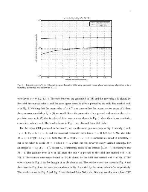
5 L=3,λ 1 =0.4,λ 2 =0.5,λ 3 =0.7,σ=1,Γ=10 10 −1 maximal remainder error level τ estimation error of x error upper bound estimation error and its upper bound of x 10 −2 10 −3 0 0.5 1 1.5 2 2.5 3 3.5 4 4.5 5 Fig. 1. Estimate error of ˆx in (18) and its upper bound in (19) using proposed robust phase unwrapping algorithm. x is a uniformly distributed real number in [0, 14). error levels τ = 0,1,2,3,4,5. The error between the estimate ˆx in (18) and the true value x is plotted by the solid line marked with × and the error upper bound in (19) is plotted by the solid line marked with ∗ in Fig. 1. Noticing that the mean value of x is 7, one can see that the reconstruction errors of x from the erroneous remainders ˜k i in (8) are small. Since the parameter x is a general real number, there is a precision error ǫ i in (2) that is reflected from error curves shown in Fig. 1 when there is no remainder errors, i.e., when τ = 0. The results shown in Fig. 1 are obtained from 200 trials. For the robust CRT proposed in Section III, we use the same parameters as in Fig. 1, namely L = 3, Γ 1 = 4, Γ 2 = 5, Γ 3 = 7, and the maximal remainder error levels τ = 0,1,2,3,4,5. We also take M = (1 + 2τ)(Γ 1 + Γ L ) + 1. Note that M = 2τ(Γ 1 + Γ L ) + 1 is sufficient as stated in Corollary 1 but is not taken to avoid M = 1 when τ = 0, which can be, however, easily verified similarly. For an integer n = n 0 Γ 1 Γ 2 · · · Γ L , integer n 0 is uniformly taken in the interval [0,M − 1] including 0 and M − 1. The estimate error of ˆn in (23) from the true n is plotted by the solid line marked with × in Fig. 2. The estimate error upper bound in (24) is plotted by the solid line marked with ∗ in Fig. 2. The errors shown in Fig. 2 can be thought of as absolute errors. The relative errors are shown in Fig. 3 and the curves in Fig. 3 are the error curves shown in Fig. 2 divided by the mean values of n, respectively. The results shown in Fig. 2 and Fig. 3 are obtained from 500 trials. One can see that our robust CRT
6 30 estimation error of n error upper bound L=3,Γ 1 =4,Γ 2 =5,Γ 3 =7, absolute errors 25 estimation error and its upper bound of n 20 15 10 5 0 0 0.5 1 1.5 2 2.5 3 3.5 4 4.5 5 maximal remainder error level τ Fig. 2. Absolute estimate error of ˆn in (23) and its upper bound in (24) using proposed robust CRT. provides small relative estimate errors when the remainders are erroneous, which the conventional CRT can not provide. Compared to the robust phase unwrapping algorithm dealing with real numbers x in Fig. 1, we are dealing with integers n here and thus there is no precision errors, i.e., ǫ i = 0, in (2) and the reconstruction (23) is accurate when there is no remainder errors, i.e., τ = 0, which can be verified from Fig. 2 and Fig. 3 where the errors are all zero when τ = 0. V. CONCLUSION In this letter, we proposed a robust phase unwrapping algorithm when the remainders have errors. Motivated from the robust phase unwrapping algorithm, we proposed a type of robust Chinese remainder theorem (CRT) for erroneous remainders. As we have mentioned before, what we want to emphasize here is that our proposed robust CRT is not trying to correct remainder errors nor precisely reconstruct an integer as in [1], [2], [3] but to reduce the reconstruction error from the conventional (non-robust) CRT. Also, what we studied in this letter is only for one integer (one x or one target) and different from the generalized CRT recently studied in [5], [6], [7] where multiple integers (multiple x or multiple targets) and sufficiently many moduli (remainder sets) are involved. Simulation results were provided to verify the theory. As a remark, this letter not only corrected an error on a result obtained in [4] but also considered a more general case for erroneous remainders than in [4].
Page 1 and 2: Phase Unwrapping and A Robust Chine
Page 3 and 4: 2 II. A ROBUST SOLUTION When the re
Page 5: 4 Since n has factors Γ i for 1
Page 9: 8 Since Γ i and Γ 1 are co-prime,

Phase Unwrapping and A Robust Chinese Remainder Theorem

You also want an ePaper? Increase the reach of your titles

Delete template?

Save as template?