1.1 Uniaxial compression in Copper (SCRIPT1): - Lammps
1.1 Uniaxial compression in Copper (SCRIPT1): - Lammps
1.1 Uniaxial compression in Copper (SCRIPT1): - Lammps

You also want an ePaper? Increase the reach of your titles
YUMPU automatically turns print PDFs into web optimized ePapers that Google loves.
3. Calculation of the stress-stra<strong>in</strong> curve and shear-stra<strong>in</strong> curve<br />
4. Dump of the atomic trayectories for visualization<br />
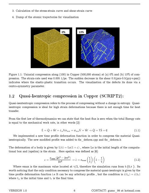
Figure <strong>1.1</strong>: <strong>Uniaxial</strong> <strong>compression</strong> along (100) <strong>in</strong> <strong>Copper</strong> (500,000 atoms) at (a) 0% and (b) 13% of <strong>compression</strong>.<br />
The stra<strong>in</strong>-rate used was 0.005 1/ps. The sudden decrease <strong>in</strong> the shear 0.5(pxx-0.5(pyy+pzz))<br />
<strong>in</strong>dicates where the elastic-plastic transition occurs. The visualization of the defects its done via a<br />
centro-symmetry parameter.<br />
1.2 Quasi-Isentropic <strong>compression</strong> <strong>in</strong> <strong>Copper</strong> (SCRIPT2):<br />
Quasi-isententropic <strong>compression</strong> refers to the process of compress<strong>in</strong>g without a change <strong>in</strong> entropy. Quasiisentropic<br />
<strong>compression</strong> is ideal for high stra<strong>in</strong> deformations because there is not enough time for heat<br />
transfer.<br />
From the first law of thermodynamics we can state that the heat flux is zero when the total Energy rate<br />
is equal to the mechanical work rate, <strong>in</strong> other words [2]:<br />
_E = _ Q + _ W = _ε α Vσ αα = σ αα<br />
_V = _ W → _ Q = T _ S = 0 (<strong>1.1</strong>)<br />
We implemented a new time profile deformation function <strong>in</strong> order to compress the material Quasiisentropically.<br />
The new modified profile was added to fix_deform.cpp and fix_deform.h<br />
The deformation of a body is given by L(t) = Lo(1 + ε) , where Lo is the <strong>in</strong>itial length of the computational<br />
box and (epsilon) is the stra<strong>in</strong> . Here epsilon was def<strong>in</strong>ed as [6]:<br />
ε = e max (2t 3 − 3τt 2 )<br />
6τ 2<br />
→ _ε = e max<br />
( t<br />
τ<br />
) (<br />
1 − t τ<br />
Where emax is the maximum value located at τ/2, therefore the simulation runs from t:{0,τ }. Its<br />
worth notic<strong>in</strong>g that the only condition necessary to compress the material quasi-isentropic is given by the<br />
time profile deformation function i.e It can be any arbritary profile , but the condition is _ε(t o ) = _ε(t f )<br />
where t o is the <strong>in</strong>itial time and t f is the f<strong>in</strong>al time.<br />
)<br />
(1.2)<br />
VERSION 1.0 6 CONTACT: gumo_99 at hotmail.com