1.1 Uniaxial compression in Copper (SCRIPT1): - Lammps
1.1 Uniaxial compression in Copper (SCRIPT1): - Lammps
1.1 Uniaxial compression in Copper (SCRIPT1): - Lammps

Create successful ePaper yourself
Turn your PDF publications into a flip-book with our unique Google optimized e-Paper software.
1<br />
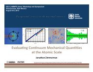
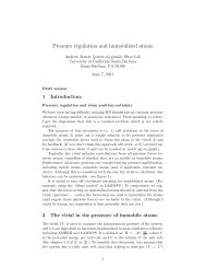
A beg<strong>in</strong>ner’s guide to the model<strong>in</strong>g of shock/uniaxial/quasi-isentropic<br />
<strong>compression</strong> us<strong>in</strong>g the LAMMPS molecular dynamics simulator By:<br />
Oscar Guerrero-Miramontes<br />
The follow<strong>in</strong>g text is a recompilation of LAMMPS [1] scripts that <strong>in</strong>tends to expla<strong>in</strong> <strong>in</strong> a nutshell the<br />
model<strong>in</strong>g of shock, uniaxial and quasi-isentropic <strong>compression</strong> us<strong>in</strong>g molecular dynamics simulations<br />
(MD). Hopefully these scripts may be useful for the MD newcomers. All the scripts provided <strong>in</strong> this<br />
text were tested us<strong>in</strong>g lammps-20Sep12 version.<br />
There is no guarantee that the scripts are fail proof or will work properly with a more recent version.<br />
<strong>1.1</strong> <strong>Uniaxial</strong> <strong>compression</strong> <strong>in</strong> <strong>Copper</strong> (<strong>SCRIPT1</strong>):<br />
The next script is useful when try<strong>in</strong>g to model uniaxial <strong>compression</strong> <strong>in</strong> BCC/FCC crystals e.g Tantalum<br />
or <strong>Copper</strong> [2,3]. The uniaxial <strong>compression</strong> can be performed along different crystalographic directions:<br />
(100),(110) and (111) to name a few. The stress-stra<strong>in</strong> curve and shear-stra<strong>in</strong> curve are plotted us<strong>in</strong>g<br />
gnuplot and the elastic-plastic transition is visualized us<strong>in</strong>g ATOMEYE [4]. The atomic <strong>in</strong>teractions are<br />
modeled us<strong>in</strong>g the embedded atom method (EAM) [5]<br />
# Isothermal <strong>Uniaxial</strong> deformation along [100],[110] or [111]<br />
# The equilibration step allows the lattice to expand to a<br />
# temperature of 300 K with a pressure of 0 kbar at each si-<br />
# mulation cell boundary. Then, the simulation cell is def-<br />
# ormed <strong>in</strong> the x-direction at a stra<strong>in</strong> rate of 0.005 1/ps,<br />
# while the lateral boundaries are controlled us<strong>in</strong>g the NVT<br />
# equations of motion to ma<strong>in</strong>ta<strong>in</strong> the length of the computa-<br />
# tional box constant. The stress and stra<strong>in</strong> values are ou-<br />
# tput to a separate file, which can be imported <strong>in</strong> a grap-<br />
# h<strong>in</strong>g application for plott<strong>in</strong>g. The cfg dump files <strong>in</strong>clude<br />
# the x, y, and z coord<strong>in</strong>ates, the centrosymmetry values, the<br />
# potential energies, and forces for each atom. This can be<br />
# directly visualized us<strong>in</strong>g AtomEye. We assume 1 timestep is<br />
# equal to 0.0005 pico-seconds<br />
# Script made by Oscar Guerrero-Miramontes<br />
# ---------- Initialize Simulation ---------------------<br />
1
clear<br />
units metal<br />
dimension 3<br />
boundary p p p<br />
atom_style atomic<br />
atom_modify map array<br />
# ---------- def<strong>in</strong>e variables ---------------------<br />
variable stemperature equal 300 # temperature <strong>in</strong> kelv<strong>in</strong><br />
variable epercentage equal 0.30 # the percentage the body is compressed<br />
variable myseed equal 12345 # the value seed for the velocity<br />
variable atomrate equal 2500 # the rate <strong>in</strong> timestep that atoms are dump as CFG<br />
variable time_step equal 0.005 # time step <strong>in</strong> pico seconds<br />
variable time_eq equal 10000 # time steps for the equlibration part<br />
variable tdamp equal "v_time_step*100" # DO NOT CHANGE<br />
variable pdamp equal "v_time_step*1000" # DO NOT CHANGE<br />
variable R equal 0.005 # ERATE here 0.005 1/ps every picosecond<br />
# time for the deformation part (DO NOT CHANGE)<br />
variable time_run equal "(v_epercentage/v_R)/v_time_step"<br />
timestep ${time_step} # DO NOT CHANGE<br />
# ---------- Create Atoms ---------------------<br />
# Create FCC lattice with x orientation along (100)<br />
# if you want to change orientation along (110) or (111)<br />
# then uncomment<br />
lattice fcc 3.615 orig<strong>in</strong> 0.0 0.0 0.0 orient x 1 0 0 orient y 0 1 0 orient z 0 0 1<br />
# lattice fcc 3.615 orig<strong>in</strong> 0.0 0.0 0.0 orient x 1 1 0 orient y 0 0 1 orient z 1 -1 0<br />
# lattice fcc 3.615 orig<strong>in</strong> 0.0 0.0 0.0 orient x 1 1 1 orient y 1 -1 0 orient z 1 1 -2<br />
region box block 0 50 0 50 0 50 units lattice<br />
create_box 1 box<br />
create_atoms 1 box<br />
# ---------- Def<strong>in</strong>e Interatomic Potential ---------------------<br />
pair_style eam/alloy<br />
pair_coeff * * Cu_mish<strong>in</strong>1.eam.alloy Cu<br />
VERSION 1.0 2 CONTACT: gumo_99 at hotmail.com
# ---------- Def<strong>in</strong>e Sett<strong>in</strong>gs ----------------------------------<br />
# "compute" Def<strong>in</strong>e a computation that will be performed on a<br />
# group of atoms. Quantities calculated by a compute are<br />
# <strong>in</strong>stantaneous values, mean<strong>in</strong>g they are calculated from<br />
# <strong>in</strong>formation about atoms on the current timestep or iteration,<br />
# though a compute may <strong>in</strong>ternally store some <strong>in</strong>formation about<br />
# a previous state of the system. Def<strong>in</strong><strong>in</strong>g a compute does not<br />
# perform a computation. Instead computes are <strong>in</strong>voked by other<br />
# LAMMPS commands as needed<br />
compute myCN all cna/atom 3.9<br />
compute myKE all ke/atom<br />
compute myPE all pe/atom<br />
# ---------- Equilibration ---------------------------------------<br />
reset_timestep 0<br />
velocity all create ${stemperature} ${myseed} mom yes rot no<br />
# The equilibration step NPT allows the lattice to expand to a<br />
# temperature of 300 K with a pressure of 0 bar at each simul-<br />
# ation cell boundary. The Tdamp and Pdamp parameter is speci-<br />
# fied <strong>in</strong> time units and determ<strong>in</strong>es how rapidly the temperatu-<br />
# re is relaxed. A good choice for many models is a Tdamp of-<br />
# around 100 timesteps and A good choice for many models is a-<br />
# Pdamp of around 1000 timesteps. Note that this is NOT the s-<br />
# ame as 1000 time units for most units sett<strong>in</strong>gs.<br />
fix equilibration all npt temp ${stemperature} ${stemperature} ${tdamp}<br />
iso 0 0 ${pdamp} drag 1<br />
# Output thermodynamics <strong>in</strong>to outputfile<br />
# for units metal, pressure is <strong>in</strong> [bars] = 100 [kPa] = 1/10000 [GPa] p2, p3, p4 are <strong>in</strong> GPa<br />
variable eq1 equal "step"<br />
variable eq2 equal "pxx/10000"<br />
variable eq3 equal "pyy/10000"<br />
variable eq4 equal "pzz/10000"<br />
variable eq5 equal "lx"<br />
variable eq6 equal "ly"<br />
variable eq7 equal "lz"<br />
variable eq8 equal "temp"<br />
variable eq9 equal "etotal"<br />
VERSION 1.0 3 CONTACT: gumo_99 at hotmail.com
fix output1 all pr<strong>in</strong>t 10 "${eq1} ${eq2} ${eq3} ${eq4} ${eq5} ${eq6} ${eq7} ${eq8} ${eq9}"<br />
file run.${stemperature}K.out screen no<br />
thermo 10<br />
thermo_style custom step pxx pyy pzz lx ly lz temp etotal<br />
# Use cfg for AtomEye (here only pr<strong>in</strong>t the coord<strong>in</strong>ates of the atoms)<br />
dump 1 all cfg ${time_eq} fcc.cu.*.cfg id type xs ys zs<br />
dump_modify 1 element Cu<br />
# RUN AT LEAST 10000 timesteps<br />
run ${time_eq}<br />
# Store f<strong>in</strong>al cell length for stra<strong>in</strong> calculations<br />
variable tmp equal "lx"<br />
variable L0 equal ${tmp}<br />
pr<strong>in</strong>t "Initial Length, L0: ${L0}"<br />
# reset<br />
unfix equilibration<br />
undump 1<br />
unfix output1<br />
# ---------- Deformation ---------------------------------<br />
reset_timestep 0<br />
# In our simulations We seek to control the lateral boundaries<br />
# Ly and Lz, i.e When the computational box is stretched,<br />
# the contraction or transverse stra<strong>in</strong> perpendicular to the<br />
# load is zero<br />
fix 1 all nvt temp ${stemperature} ${stemperature} ${tdamp} drag 0.0<br />
fix 2 all deform 1 x erate -${R} units box remap x<br />
# IMPORTANT NOTE: When non-equilibrium MD (NEMD) simulations are<br />
# performed us<strong>in</strong>g this fix, the option "remap v" should normally<br />
# be used. This is because fix nvt/sllod adjusts the atom positions<br />
# and velocities to <strong>in</strong>duce a velocity profile that matches the<br />
# chang<strong>in</strong>g box size/shape. Thus atom coord<strong>in</strong>ates should NOT be<br />
# remapped by fix deform, but velocities SHOULD be when atoms cross<br />
# periodic boundaries, s<strong>in</strong>ce that is consistent with ma<strong>in</strong>ta<strong>in</strong><strong>in</strong>g<br />
# the velocity profile already created by fix nvt/sllod. LAMMPS<br />
# will warn you if the remap sett<strong>in</strong>g is not consistent with fix nvt/sllod.<br />
VERSION 1.0 4 CONTACT: gumo_99 at hotmail.com
# Output stra<strong>in</strong> and stress <strong>in</strong>fo to file<br />
# for units metal, pressure is <strong>in</strong> [bars] = 100 [kPa] = 1/10000 #[GPa] pxx, pyy, pzz<br />
# are <strong>in</strong> GPa<br />
variable stra<strong>in</strong> equal "-(lx - v_L0)/v_L0"<br />
variable shear equal "0.5*(pxx/10000 - 0.5*(pyy/10000 + pzz/10000))"<br />
variable tstep equal "step"<br />
variable mypxx equal "pxx/10000"<br />
variable mypyy equal "pyy/10000"<br />
variable mypzz equal "pzz/10000"<br />
variable mylx equal "lx"<br />
variable myly equal "ly"<br />
variable mylz equal "lz"<br />
variable mytemp equal "temp"<br />
fix def1 all pr<strong>in</strong>t 10 "${stra<strong>in</strong>} ${mypxx} ${mypyy} ${mypzz} ${shear} ${mylx} ${myly} ${mylz}<br />
${mytemp}" file stress.${stemperature}K.${epercentage}e.out screen no<br />
# Use cfg for AtomEye<br />
dump 1 all cfg ${atomrate} dump._*.cfg id type xs ys zs c_myPE c_myKE c_myCN fx fy fz<br />
dump_modify 1 element Cu<br />
# Display thermo<br />
variable thermostep equal "v_time_run/10"<br />
thermo ${thermostep}<br />
thermo_style custom "v_stra<strong>in</strong>" pxx pyy pzz lx ly lz temp etotal pe ke<br />
run ${time_run}<br />
unfix def1<br />
unfix 1<br />
unfix 2<br />
# SAVE THE DATA OF THE CALCULATION OR ELSE YOU NEED TO START OVER<br />
write_restart restart.equil<br />
# SIMULATION DONE<br />
clear<br />
pr<strong>in</strong>t "creo ya esta =)"<br />
The steps taken for the <strong>Uniaxial</strong> <strong>compression</strong> of copper were the follow<strong>in</strong>g :<br />
1. Equilibration of the system<br />
2. Deformation of the computational box along the x-direction<br />
VERSION 1.0 5 CONTACT: gumo_99 at hotmail.com
3. Calculation of the stress-stra<strong>in</strong> curve and shear-stra<strong>in</strong> curve<br />
4. Dump of the atomic trayectories for visualization<br />
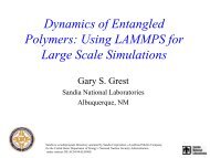
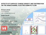
Figure <strong>1.1</strong>: <strong>Uniaxial</strong> <strong>compression</strong> along (100) <strong>in</strong> <strong>Copper</strong> (500,000 atoms) at (a) 0% and (b) 13% of <strong>compression</strong>.<br />
The stra<strong>in</strong>-rate used was 0.005 1/ps. The sudden decrease <strong>in</strong> the shear 0.5(pxx-0.5(pyy+pzz))<br />
<strong>in</strong>dicates where the elastic-plastic transition occurs. The visualization of the defects its done via a<br />
centro-symmetry parameter.<br />
1.2 Quasi-Isentropic <strong>compression</strong> <strong>in</strong> <strong>Copper</strong> (SCRIPT2):<br />
Quasi-isententropic <strong>compression</strong> refers to the process of compress<strong>in</strong>g without a change <strong>in</strong> entropy. Quasiisentropic<br />
<strong>compression</strong> is ideal for high stra<strong>in</strong> deformations because there is not enough time for heat<br />
transfer.<br />
From the first law of thermodynamics we can state that the heat flux is zero when the total Energy rate<br />
is equal to the mechanical work rate, <strong>in</strong> other words [2]:<br />
_E = _ Q + _ W = _ε α Vσ αα = σ αα<br />
_V = _ W → _ Q = T _ S = 0 (<strong>1.1</strong>)<br />
We implemented a new time profile deformation function <strong>in</strong> order to compress the material Quasiisentropically.<br />
The new modified profile was added to fix_deform.cpp and fix_deform.h<br />
The deformation of a body is given by L(t) = Lo(1 + ε) , where Lo is the <strong>in</strong>itial length of the computational<br />
box and (epsilon) is the stra<strong>in</strong> . Here epsilon was def<strong>in</strong>ed as [6]:<br />
ε = e max (2t 3 − 3τt 2 )<br />
6τ 2<br />
→ _ε = e max<br />
( t<br />
τ<br />
) (<br />
1 − t τ<br />
Where emax is the maximum value located at τ/2, therefore the simulation runs from t:{0,τ }. Its<br />
worth notic<strong>in</strong>g that the only condition necessary to compress the material quasi-isentropic is given by the<br />
time profile deformation function i.e It can be any arbritary profile , but the condition is _ε(t o ) = _ε(t f )<br />
where t o is the <strong>in</strong>itial time and t f is the f<strong>in</strong>al time.<br />
)<br />
(1.2)<br />
VERSION 1.0 6 CONTACT: gumo_99 at hotmail.com
The modification of LAMMPS source code to add the new deformation time profile is easy. In older<br />
versions of LAMMPS it was neccesary to HACK the code and modify fix_deform.cpp, but the recent<br />
version of LAMMPS <strong>in</strong>clude a new fix deform style "variable" : The variable style changes the specified<br />
box length dimension by evaluat<strong>in</strong>g a variable, which presumably is a function of time. I decided to<br />
implement my own HACK rather than use the fix deform "variable" style.<br />
First I added a new variable (tau) to fix_deform.h , then we replaced the TRATE L(t) profile :<br />
set[i].lo_stop = 0.5*(set[i].lo_start+set[i].hi_start) -<br />
0.5*((set[i].hi_start-set[i].lo_start) *<br />
exp(set[i].rate*delt)); set[i].hi_stop = 0.5*(set[i].lo_start+set[i].hi_start) +<br />
0.5*((set[i].hi_start-set[i].lo_start) * exp(set[i].rate*delt));<br />
to the new form given <strong>in</strong> equation (1.2) :<br />
set[i].lo_stop = 0.5*(set[i].lo_start+set[i].hi_start)<br />
-0.5*((set[i].hi_start-set[i].lo_start) *<br />
(1 + pow(set[i].tau,-2)*0.1666*set[i].rate*(2*pow(delt,3)-3*set[i].tau*pow(delt,2))));<br />
set[i].hi_stop = 0.5*(set[i].lo_start+set[i].hi_start) +<br />
0.5*((set[i].hi_start-set[i].lo_start) *<br />
(1 + pow(set[i].tau,-2)*0.1666*set[i].rate*(2*pow(delt,3)-3*set[i].tau*pow(delt,2))));<br />
F<strong>in</strong>aly I renamed TRATE L(t) profile to QRATE . After the modifications to fix_deform.cpp , and<br />
fix_deform.h then LAMMPS was recompiled e.g make openmpi. If LAMMPS compiles successfully,<br />
then the new profile is ready to RUN .<br />
Now I will show a LAMMPS script that implements Quasi-isentropic <strong>compression</strong> <strong>in</strong> <strong>Copper</strong>:<br />
# Quasi Isentropic deformation <strong>Copper</strong> along [100], [110] or [111]<br />
# The equilibration step allows the lattice to expand to a temperature of 300 K with a<br />
# pressure of 0 kbar at each simulation cell boundary. Then, the simulation cell is<br />
# deformed <strong>in</strong> the x-direction at, while the lateral boundaries are controlled us<strong>in</strong>g<br />
# the NVT equations of motion to manta<strong>in</strong> the lenght of the computational box constant.<br />
# The stress and stra<strong>in</strong> values are output to a separate file, which can be imported <strong>in</strong><br />
# a graph<strong>in</strong>g application for plott<strong>in</strong>g. The cfg dump files <strong>in</strong>clude the x, y, and z<br />
# coord<strong>in</strong>ates, the centrosymmetry values, the potential energies, and forces for each atom.<br />
# This can be directly visualized us<strong>in</strong>g AtomEye We assume 1 timestep is equal to 0.0005<br />
# pico-seconds<br />
# SCRIPT MADE BY OSCAR GUERRERO-MIRAMONTES<br />
# ---------- Initialize Simulation ---------------------<br />
clear<br />
units metal<br />
dimension 3<br />
VERSION 1.0 7 CONTACT: gumo_99 at hotmail.com
oundary p p p<br />
atom_style atomic<br />
atom_modify map array<br />
# ---------- def<strong>in</strong>e variables ---------------------<br />
variable stemperature equal 300 # temperature <strong>in</strong> kelv<strong>in</strong><br />
variable epercentage equal 0.19 # the percentage the body is compressed<br />
variable myseed equal 12345 # the value seed for the velocity<br />
variable atomrate equal 250 # the rate <strong>in</strong> timestep that atoms are dump as CFG<br />
variable time_step equal 0.0005 # time step <strong>in</strong> pico seconds (CHANGE THIS VALUE)<br />
variable tau equal 5<br />
# quasi-isentropic scheme f<strong>in</strong>al run time (<strong>in</strong> time UNITS)<br />
variable time_eq equal 10000 # time steps for the equlibration part<br />
variable time_nvt equal 5000 # time steps for the NVT (NUCLEATION DEFECTS)<br />
variable tdamp equal "v_time_step*100" # DO NOT CHANGE<br />
variable pdamp equal "v_time_step*1000" # DO NOT CHANGE<br />
variable R equal "(v_epercentage/0.165)/v_tau" # Compress rate <strong>in</strong> EMAX<br />
variable time_run equal "v_tau/v_time_step" # time step for the deformation part<br />
timestep ${time_step} # DO NOT CHANGE<br />
# ---------- Create Atoms ---------------------<br />
lattice fcc 3.615 orig<strong>in</strong> 0.0 0.0 0.0 orient x 1 0 0 orient y 0 1 0 orient z 0 0 1<br />
# lattice fcc 3.615 orig<strong>in</strong> 0.0 0.0 0.0 orient x 1 1 0 orient y 0 0 1 orient z 1 -1 0<br />
# lattice fcc 3.615 orig<strong>in</strong> 0.0 0.0 0.0 orient x 1 1 1 orient y 1 -1 0 orient z 1 1 -2<br />
region box block 0 50 0 50 0 50 units lattice<br />
create_box 1 box<br />
create_atoms 1 box<br />
# ---------- Def<strong>in</strong>e Interatomic Potential ---------------------<br />
pair_style eam/alloy<br />
pair_coeff * * Cu_mish<strong>in</strong>1.eam.alloy Cu<br />
# ---------- Def<strong>in</strong>e Sett<strong>in</strong>gs ----------------------------------<br />
# "compute" Def<strong>in</strong>e a computation that will be performed on a group of atoms. Quantities<br />
# calculated by a compute are <strong>in</strong>stantaneous values, mean<strong>in</strong>g they are calculated from<br />
# <strong>in</strong>formation about atoms on the current timestep or iteration, though a compute may<br />
# <strong>in</strong>ternally store some <strong>in</strong>formation about a previous state of the system. Def<strong>in</strong><strong>in</strong>g a<br />
# compute does not perform a computation.Instead computes are <strong>in</strong>voked by other LAMMPS<br />
# commands as needed<br />
VERSION 1.0 8 CONTACT: gumo_99 at hotmail.com
compute myCN all cna/atom 3.8<br />
compute myKE all ke/atom<br />
compute myPE all pe/atom<br />
# ---------- Equilibration ---------------------------------------<br />
reset_timestep 0<br />
velocity all create ${stemperature} ${myseed} mom yes rot no<br />
fix equilibration all npt temp ${stemperature} ${stemperature} ${tdamp}<br />
iso 0 0 ${pdamp} drag 0.0<br />
# Output thermodynamics <strong>in</strong>to outputfile<br />
# for units metal, pressure is <strong>in</strong> [bars] = 100 [kPa] = 1/10000 [GPa]<br />
# p2, p3, p4 are <strong>in</strong> GPa<br />
variable eq1 equal "step"<br />
variable eq2 equal "pxx/10000"<br />
variable eq3 equal "pyy/10000"<br />
variable eq4 equal "pzz/10000"<br />
variable eq5 equal "lx"<br />
variable eq6 equal "ly"<br />
variable eq7 equal "lz"<br />
variable eq8 equal "temp"<br />
variable eq9 equal "etotal"<br />
fix output1 all pr<strong>in</strong>t 10 "${eq1} ${eq2} ${eq3} ${eq4} ${eq5} ${eq6} ${eq7} ${eq8} ${eq9}"<br />
file run.${stemperature}K.out screen no<br />
thermo 10<br />
thermo_style custom step pxx pyy pzz lx ly lz temp etotal<br />
# Use cfg for AtomEye (here only pr<strong>in</strong>t the coord<strong>in</strong>ates of the atoms)<br />
dump 1 all cfg ${time_eq} fcc.copper.*.cfg id type xs ys zs<br />
dump_modify 1 element Cu<br />
# RUN AT LEAST 10000 timesteps<br />
run ${time_eq}<br />
# Store f<strong>in</strong>al cell length for stra<strong>in</strong> calculations<br />
variable tmp equal "lx"<br />
variable L0 equal ${tmp}<br />
pr<strong>in</strong>t "Initial Length, L0: ${L0}"<br />
#reset<br />
unfix equilibration<br />
undump 1<br />
VERSION 1.0 9 CONTACT: gumo_99 at hotmail.com
unfix output1<br />
# ---------- Deformation ---------------------------------<br />
reset_timestep 0<br />
# QRATE IS OUR MODIFIED FUNCTIONAL FORM AND IS A LAMMPS HACK<br />
fix 1 all nve<br />
fix 2 all deform 1 x qrate ${R} ${tau} units box remap x<br />
# Output stra<strong>in</strong> and stress <strong>in</strong>fo to file<br />
# for units metal, pressure is <strong>in</strong> [bars] = 100 [kPa] = 1/10000 [GPa]<br />
# pxx, pyy, pzz are <strong>in</strong> GPa<br />
variable stra<strong>in</strong> equal "-(lx - v_L0)/v_L0"<br />
variable shear equal "0.5*(pxx/10000 - 0.5*(pyy/10000 + pzz/10000))"<br />
variable tstep equal "step"<br />
variable out1 equal "v_stra<strong>in</strong>"<br />
variable out2 equal "pxx/10000"<br />
variable out3 equal "pyy/10000"<br />
variable out4 equal "pzz/10000"<br />
variable out5 equal "v_shear"<br />
variable out6 equal "lx"<br />
variable out7 equal "ly"<br />
variable out8 equal "lz"<br />
variable out9 equal "temp"<br />
variable out10 equal "vol"<br />
# Volume Angstroms^3<br />
variable out11 equal "etotal" # ENERGY IN EV<br />
variable out12 equal "press/10000" # PRESSURE IN GPa<br />
variable out13 equal "((press/10000)*vol)/160.21" # MECHANICAL WORK W = PV <strong>in</strong> EV<br />
fix def1 all pr<strong>in</strong>t 1 "${tstep} ${out2} ${out3} ${out4} ${out5} ${out6} ${out7}<br />
${out8} ${out9} ${out10} ${out11} ${out12}" file stress.${stemperature}K.${epercentage}e.out<br />
screen no<br />
# Display thermo<br />
variable thermostep equal "v_time_run/10"<br />
thermo ${thermostep}<br />
thermo_style custom "v_stra<strong>in</strong>" pxx pyy pzz lx ly lz temp etotal pe ke<br />
# Use cfg for AtomEye (here only pr<strong>in</strong>t the coord<strong>in</strong>ates of the atoms)<br />
dump 1 all cfg ${atomrate} dump.copper.*.cfg id type xs ys zs<br />
dump_modify 1 element Cu<br />
VERSION 1.0 10 CONTACT: gumo_99 at hotmail.com
un ${time_run}<br />
unfix def1<br />
unfix 1<br />
unfix 2<br />
# SIMULATION DONE<br />
clear<br />
pr<strong>in</strong>t "creo ya esta =)"<br />
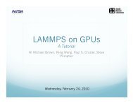
The above script first equlibrates the systems to a temperature of 300K , and next Quasi-isentropically<br />
compress the material up to 19% <strong>in</strong> 5 picoseconds. We can make a plot of the total energy rate E _ vs<br />
the mechanical work rate W _ = P V _ . As the next figure shows (figure 1.2), all the Energy transfer to<br />
mechanical work i.e E _ = W _ , thus the heat flux Q _ equals zero and the change of entropy with time is<br />
zero S _ = 0<br />
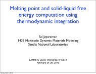
Figure 1.2: <strong>Uniaxial</strong> Quasi-isentropic <strong>compression</strong> along (100) <strong>in</strong> <strong>Copper</strong> (500,000 atoms). The image<br />
to the left show the Shear τ = 0.5(Pxx − 0.5(Pyy + Pzz)) and the nucleation of defects us<strong>in</strong>g a centrosymmetry<br />
analysis. The right image show the energy rate E _ (black l<strong>in</strong>e) vs _W = P V _ (cyan l<strong>in</strong>e). As is<br />
evident E _ = W _ and thus the S _ = 0<br />
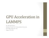
Now I will show the time profile of pressure,temperature and stra<strong>in</strong> rate obta<strong>in</strong>ed:<br />
VERSION 1.0 11 CONTACT: gumo_99 at hotmail.com
Figure 1.3: <strong>Uniaxial</strong> Quasi-isentropic <strong>compression</strong> along (100) <strong>in</strong> <strong>Copper</strong> (500,000 atoms). The image<br />
show the profiles of pressure, temperature, stra<strong>in</strong>-rate and volume obta<strong>in</strong>ed after runn<strong>in</strong>g the modified<br />
HACK version of LAMMPS<br />
1.3 Shock Compression <strong>in</strong> Niquel (SCRIPT3):<br />
Consider a cont<strong>in</strong>uous block of material of constant cross-section A. A piston drives <strong>in</strong>to the material<br />
with a velocity U p . In the situation be<strong>in</strong>g considered here, the piston is travell<strong>in</strong>g at a constant velocity.<br />
Therefore the material beh<strong>in</strong>d the shock is travell<strong>in</strong>g at the same velocity as the piston. From figure 1.4<br />
and 1.5 it can be seen that the motion of the piston causes an <strong>in</strong>crease <strong>in</strong> the density of the material<br />
ahead of it, as the material is ’gathered up’. The action of the piston, which causes the material to beg<strong>in</strong><br />
mov<strong>in</strong>g, and the resultant <strong>in</strong>crease <strong>in</strong> density causes a shock to travel forward at velocity U s .<br />
Figure 1.4: Schematic of shock propagation<br />
VERSION 1.0 12 CONTACT: gumo_99 at hotmail.com
Figure 1.5: Schematic of a simple piston driven shock. The piston drives <strong>in</strong>to the material from the left.<br />
Each horizontal row is a snapshot of the system at some time. The <strong>in</strong>itial state is at the bottom of the<br />
figure, and time <strong>in</strong>creases up the figure. Thus it can be seen that the slope of the arrow labelled Up<br />
gives the velocity of the piston, and that labelled Us gives the velocity of the shock front runn<strong>in</strong>g ahead<br />
<strong>in</strong>to the material at rest.<br />
Now I will present a LAMMPS’s Script that simulates a piston drive shock as described <strong>in</strong> the above<br />
figure. In this example we choose FCC Niquel [7,8]. Descriptions of the physics of shock and calculation<br />
of the shock speed U s are given <strong>in</strong> many texts. The <strong>in</strong>terested reader is referred to [9,10,11,12,13,14].<br />
# SCRIPT MADE BY: OSCAR GUERRERO<br />
# ---------- Initialize Simulation ---------------------<br />
clear<br />
units metal<br />
dimension 3<br />
boundary p p p<br />
atom_style atomic<br />
atom_modify map array<br />
# ---------- def<strong>in</strong>e variables ---------------------<br />
variable stemperature equal 5 # temperature <strong>in</strong> kelv<strong>in</strong><br />
variable alattice equal 3.520 # lattice constant (unit A)<br />
variable myseed equal 12345 # the value seed for the velocity<br />
variable xmax equal 40 # size <strong>in</strong> the x-direction<br />
variable ymax equal 40 # size <strong>in</strong> the y-direction<br />
VERSION 1.0 13 CONTACT: gumo_99 at hotmail.com
variable zmax equal 70 # size <strong>in</strong> the z-direction<br />
variable time_step equal 0.001 # time step <strong>in</strong> pico seconds<br />
variable time_eq equal 1000 # time steps for the equlibration part<br />
variable time_shock equal 15000 # time steps for the piston<br />
variable vpiston equal 1.300 # piston speed <strong>in</strong> (km/s) multiply by ten to obta<strong>in</strong> (A/ps)<br />
variable Nevery equal 10 # use <strong>in</strong>put values every this many timesteps<br />
variable Nrepeat equal 5 # number of times to use <strong>in</strong>put values for calculat<strong>in</strong>g<br />
variable Nfreq equal 100 # calculate averages every this many timesteps<br />
variable deltaz equal 3 # thickness of spatial b<strong>in</strong>s <strong>in</strong> dim (distance units)<br />
variable atomrate equal 100 # the rate <strong>in</strong> timestep that atoms are dump as CFG<br />
variable tdamp equal "v_time_step*100" # DO NOT CHANGE<br />
variable pdamp equal "v_time_step*1000" # DO NOT CHANGE<br />
# DO NOT CHANGE<br />
variable Up equal "10*v_vpiston"<br />
timestep ${time_step}<br />
# ---------- Create Atoms ---------------------<br />
lattice fcc ${alattice} orig<strong>in</strong> 0.0 0.0 0.0 orient x 1 0 0 orient y 0 1 0 orient z 0 0 1<br />
# lattice fcc ${alattice} orig<strong>in</strong> 0.0 0.0 0.0 orient x 1 1 0 orient y 0 0 1 orient z 1 -1 0<br />
# lattice fcc ${alattice} orig<strong>in</strong> 0.0 0.0 0.0 orient x 1 1 1 orient y 1 -1 0 orient z 1 1 -2<br />
# the create box commands create_box natoms idname, where natoms is the number of atoms type<br />
# <strong>in</strong> the simulation box for this case we only have one type of atoms<br />
# you can use the command "set" to set the different region of atoms to different Ntype<br />
# the command "set" is very useful examples: "set group piston type 1"<br />
# def<strong>in</strong>e size of the simulation box<br />
region sim_box block 0 ${xmax} 0 ${ymax} 0 ${zmax} units lattice<br />
create_box 2 sim_box<br />
# def<strong>in</strong>e atoms <strong>in</strong> a small region<br />
region atom_box block 0 ${xmax} 0 ${ymax} 0 ${zmax}<br />
create_atoms 1 region atom_box<br />
# def<strong>in</strong>e a group for the atom_box region<br />
group atom_box region atom_box<br />
region piston block INF INF INF INF INF 4<br />
region bulk block INF INF INF INF 4 INF<br />
group piston<br />
group bulk<br />
region piston<br />
region bulk<br />
VERSION 1.0 14 CONTACT: gumo_99 at hotmail.com
set group piston type 1<br />
set group bulk type 2<br />
# ---------- Def<strong>in</strong>e Interatomic Potential ---------------------<br />
pair_style eam/fs<br />
pair_coeff * * Ni.lammps.eam Ni Ni<br />
mass 1 58.70<br />
mass 2 58.70<br />
compute myCN bulk cna/atom fcc<br />
compute myKE bulk ke/atom<br />
compute myPE bulk pe/atom<br />
compute myCOM bulk com<br />
compute peratom bulk stress/atom<br />
compute vz bulk property/atom vz<br />
# ------------ Equilibrate ---------------------------------------<br />
reset_timestep 0<br />
# Now, assign the <strong>in</strong>itial velocities us<strong>in</strong>g Maxwell-Boltzmann distribution<br />
velocity atom_box create ${stemperature} ${myseed} rot yes dist gaussian<br />
fix equilibration bulk npt temp ${stemperature} ${stemperature} ${tdamp}<br />
iso 0 0 ${pdamp} drag 1<br />
variable eq1 equal "step"<br />
variable eq2 equal "pxx/10000"<br />
variable eq3 equal "pyy/10000"<br />
variable eq4 equal "pzz/10000"<br />
variable eq5 equal "lx"<br />
variable eq6 equal "ly"<br />
variable eq7 equal "lz"<br />
variable eq8 equal "temp"<br />
variable eq9 equal "etotal"<br />
fix output1 bulk pr<strong>in</strong>t 10 "${eq1} ${eq2} ${eq3} ${eq4} ${eq5} ${eq6} ${eq7} ${eq8} ${eq9}"<br />
file run.out screen no<br />
thermo 10<br />
thermo_style custom step pxx pyy pzz lx ly lz temp etotal<br />
VERSION 1.0 15 CONTACT: gumo_99 at hotmail.com
un ${time_eq}<br />
unfix equilibration<br />
unfix output1<br />
# -------------- Shock -------------------------------------------<br />
change_box all boundary p p s<br />
reset_timestep 0<br />
# WE CREATE A PISTON USING A FEW LAYERS OF ATOMS AND THEN WE GIVE IT<br />
# A CONSTANT POSTIVE SPEED. YOU COULD ALSO USE LAMMPS' FIX WALL/PISTON COMMAND<br />
fix 1 all nve<br />
velocity piston set 0 0 v_Up sum no units box<br />
fix 2 piston setforce 0.0 0.0 0.0<br />
# WE CREATE BINS IN ORDER TO TRACK THE PASSING OF THE SHOCKWAVE<br />
fix density_profile bulk ave/spatial ${Nevery} ${Nrepeat} ${Nfreq} z lower ${deltaz}<br />
density/mass file denz.profile units box<br />
variable temp atom c_myKE/(1.5*8.61e-5)<br />
fix temp_profile bulk ave/spatial ${Nevery} ${Nrepeat} ${Nfreq} z lower ${deltaz}<br />
v_temp file temp.profile units box<br />
variable meanpress atom -(c_peratom[1]+c_peratom[2]+c_peratom[3])/3<br />
fix pressure_profile bulk ave/spatial ${Nevery} ${Nrepeat} ${Nfreq} z lower ${deltaz}<br />
v_meanpress units box file pressure.profile<br />
fix velZ_profile bulk ave/spatial ${Nevery} ${Nrepeat} ${Nfreq} z lower ${deltaz}<br />
c_vz units box file velocityZcomp.profile<br />
variable eq1 equal "step"<br />
variable eq2 equal "pxx/10000"<br />
variable eq3 equal "pyy/10000"<br />
variable eq4 equal "pzz/10000"<br />
variable eq5 equal "lx"<br />
variable eq6 equal "ly"<br />
variable eq7 equal "lz"<br />
variable eq8 equal "temp"<br />
variable eq9 equal "etotal"<br />
variable eq10 equal "c_myCOM[3]"<br />
fix shock bulk pr<strong>in</strong>t 10 "${eq1} ${eq2} ${eq3} ${eq4} ${eq5} ${eq6} ${eq7} ${eq8} ${eq9}<br />
${eq10}" file run.${stemperature}K.out screen no<br />
VERSION 1.0 16 CONTACT: gumo_99 at hotmail.com
thermo 10<br />
thermo_style custom step pxx pyy pzz lx ly lz temp etotal c_myCOM[3]<br />
#Use cfg for AtomEye<br />
dump 1 all cfg ${atomrate} dump._*.cfg id type xs ys zs c_myPE c_myKE c_myCN<br />
dump_modify 1 element Cu Ni<br />
run ${time_shock}<br />
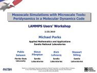
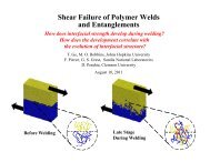
Figure 1.6: NEMD shock <strong>compression</strong> simulation <strong>in</strong> Niquel us<strong>in</strong>g the EAM potential <strong>in</strong>teraction and a<br />
piston speed Up = 1.3 km/s. Figure a). shows the system at the begg<strong>in</strong><strong>in</strong>g and figure b). Shows the<br />
nucleation of defects due to the pass<strong>in</strong>g of the shockwave.<br />
VERSION 1.0 17 CONTACT: gumo_99 at hotmail.com
The steps taken for the Shock <strong>compression</strong> of Niquel were the follow<strong>in</strong>g :<br />
1. Equilibration of the system<br />
2. Def<strong>in</strong>e a fixed layer of atoms to act as a Piston<br />
3. Periodic boundary conditions are applied <strong>in</strong> the x and y directions. Boundaries are free <strong>in</strong> the z<br />
direction<br />
4. Def<strong>in</strong>e BINS to track the pass<strong>in</strong>g of the shockwave<br />
5. Dump of the atomic trayectories for visualization<br />
Acknowledgement<br />
I would like to thank the LAMMPS community for the great FeedBack and discussions that made<br />
it possible to complete this brief tutorial. I would also like to thank the follow<strong>in</strong>g people for their<br />
contribution of ideas: Steve Plimpton, Nigel Park, Ray Shan, Jonathan Zimmerman, Vishnu Wakof,<br />
Anirban Dhar, Axel Kohlmeyer. Selesta Oxem, Rajdeep Behera, Paul Swa<strong>in</strong>, Gildardo Rivas, and Mark<br />
Tschopp<br />
VERSION 1.0 18 CONTACT: gumo_99 at hotmail.com
REFERENCES<br />
[1] S.J. Plimpton, Fast parallel algorithms for short-range molecular dynamics, J Comp Phys 117 (1995)<br />
1.<br />
[2] O. Guerrero, Pressure <strong>in</strong>duced dynamical <strong>in</strong>stabilities <strong>in</strong> body center cubic crystals, Thesis, M.S.,<br />
UTEP, 2010, p. 35.<br />
[3] Yuhang J<strong>in</strong>g; Q<strong>in</strong>gyuan Meng; Yufei Gao, Molecular dynamics simulation on the buckl<strong>in</strong>g behavior<br />
of silicon nanowires under uniaxial <strong>compression</strong>, Computational Materials Science (April 2009), 45<br />
(2), pg. 321-326<br />
[4] J. Li, AtomEye: an efficient atomistic configuration viewer, Modell<strong>in</strong>g Simul. Mater. Sci. Eng. 11<br />
(2003) 173.<br />
[5] Y. Mish<strong>in</strong>, M. J. Mehl, D. A. Papaconstantopoulos, A. F. Voter and J. D. Kress, Structural stability<br />
and lattice defects <strong>in</strong> copper: Ab <strong>in</strong>itio, tight-b<strong>in</strong>d<strong>in</strong>g, and embedded-atom calculations, Phys. Rev.<br />
B 63, 224106 (2001)<br />
[6] R. Ravelo, B.L. Holian, c T.C. Germann, High stra<strong>in</strong> rates effects <strong>in</strong> quasi-isentropic <strong>compression</strong> of<br />
solids, AIP Conf. Proc. 1195 (2009).<br />
[7] H N Jarmakani, E M Br<strong>in</strong>ga, P Erhart, B A Rem<strong>in</strong>gton, Y M Wang, N Q Vo, M A Meyers, Molecular<br />
dynamics simulations of shock <strong>compression</strong> of nickel: From monocrystals to nanocrystals, Acta<br />
Materialia 56 (2008) 5584-5604<br />
[8] Y. Mish<strong>in</strong>, D. Farkas, M.J. Mehl, and D.A. Papaconstantopolous, Interatomic Potentials for<br />
Monoatomic Metals from Experimental Data and ab <strong>in</strong>itio calculations, Phys. Rev. B 59, 3393<br />
(1999)<br />
[9] E.M. Br<strong>in</strong>ga, J.U. Cazamias, P. Erhart, J. Stolken, N. Tanushev, B.D. Wirth, et al., Atomistic shock<br />
Hugoniot simulation of s<strong>in</strong>gle-crystal copper, J. Appl. Phys. 96 (2004) 3793.<br />
[10] Brad Lee Holian, Plasticity Induced by Shock Waves <strong>in</strong> Nonequilibrium Molecular-Dynamics Simulations,<br />
Proceed<strong>in</strong>gs of APS Topical Group on Shock Compression, Amherst, MA, 27 July - August<br />
(1997)<br />
[11] Lan He, Thomas D. Sewell, and Donald L. Thompson, Molecular dynamics simulations of shock<br />
waves <strong>in</strong> oriented nitromethane s<strong>in</strong>gle crystals, J. Chem. Phys. 134, 124506 (2011)<br />
[12] W. J. Macquorn Rank<strong>in</strong>e. On the thermodynamic theory of waves of f<strong>in</strong>ite longitud<strong>in</strong>al disturbance.<br />
Philosophical Transactions of the Royal Society of London, 160:277-288, January 1870.<br />
19
[13] A. Siavosh-Haghighi, R. Dawes, T. D. Sewell, and D. L. Thompson, Shock-<strong>in</strong>duced melt<strong>in</strong>g of<br />
(100)-oriented nitromethane: Energy partition<strong>in</strong>g and vibrational mode heat<strong>in</strong>g, J. Chem. Phys.<br />
131, 064503 (2009).<br />
[14] H. Hugoniot. Propagation des mouvements dans les corps et specialement dans les gaz parfaits.<br />
Journal de lEcole Polytechnique, 57:3-98, 1887.<br />
VERSION 1.0 20 CONTACT: gumo_99 at hotmail.com