Calculating the Electrostatic Potential Energy Based on ... - Lammps

<strong>Calculating</strong> <strong>the</strong> <strong>Electrostatic</strong> <strong>Potential</strong> <strong>Energy</strong> <strong>Based</strong> on <strong>the</strong> Madelung Constant for B1
Crystal Lattice in LAMMPS with PPPM
Jan-Michael Carrillo
janmikel@gmail.com
November 23,2011
Introduction
This is a series of LAMMPS run that calculates <strong>the</strong> potential energy from a system that is arranged in a B1 lattice
structure. The B1 structure is similar to <strong>the</strong> crystal structure of NaCl. The simulation box consists of charges arranged in
<strong>the</strong> B1 lattice structure with separation distance r o of 2.0 hence <strong>the</strong> lattice constant a is 4.0.
The objective is to test <strong>the</strong> accuracy of <strong>the</strong> PPPM 1 implementation in LAMMPS by comparing <strong>the</strong> value of <strong>the</strong>
electrostatic potential energy calculated from <strong>the</strong> analytical Madelung constant from <strong>the</strong> normalized electrostatic energy
that is calculated by LAMMPS with PPPM.
Method
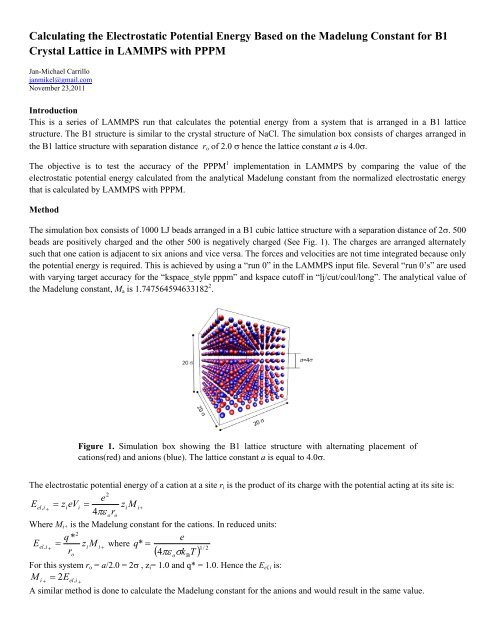
The simulation box consists of 1000 LJ beads arranged in a B1 cubic lattice structure with a separation distance of 2. 500
beads are positively charged and <strong>the</strong> o<strong>the</strong>r 500 is negatively charged (See Fig. 1). The charges are arranged alternately
such that one cation is adjacent to six anions and vice versa. The forces and velocities are not time integrated because only
<strong>the</strong> potential energy is required. This is achieved by using a “run 0” in <strong>the</strong> LAMMPS input file. Several “run 0’s” are used
with varying target accuracy for <strong>the</strong> “kspace_style pppm” and kspace cutoff in “lj/cut/coul/long”. The analytical value of
<strong>the</strong> Madelung constant, M a is 1.747564594633182 2 .
Figure 1. Simulation box showing <strong>the</strong> B1 lattice structure with alternating placement of
cations(red) and anions (blue). The lattice constant a is equal to 4.0.
The electrostatic potential energy of a cation at a site r i is <strong>the</strong> product of its charge with <strong>the</strong> potential acting at its site is:
2
e
Eel,
i
z
ieVi
ziM
i
4
oro
Where M i+ is <strong>the</strong> Madelung constant for <strong>the</strong> cations. In reduced units:
2
q *
e
Eel,
i
z
iM
i
where q*
r
4 k T
1/
o
o
2
For this system r o = a/2.0 = 2 , z i = 1.0 and q* = 1.0. Hence <strong>the</strong> E el,i is:
2
M i
E
el , i
B
A similar method is done to calculate <strong>the</strong> Madelung constant for <strong>the</strong> anions and would result in <strong>the</strong> same value.

M i
2 E
el , i
For an ionic solid, <strong>the</strong> sum of contributions of cations and anions of a crystal would <strong>the</strong>n be <strong>the</strong> sum of <strong>the</strong> partial
Madulung constants of cation and anion subarrays 3 . Hence <strong>the</strong> total Madelung constant is,
M
a
M
i
M
i
2 E
el , i
+ 2 E
el ,
= 4E i el , i
where E
el , i
would be <strong>the</strong> normalize potential energy that will be outputted by
LAMMPS.
Thus, in order to compare <strong>the</strong> results of <strong>the</strong> “run 0” LAMMPS run with <strong>the</strong> analytical expected value of <strong>the</strong> electrostatic
energy, we should divide <strong>the</strong> analytical Madelung constant, M a by 4 ( E M / 4 ). The expected normalized
electrostatic potential energy up to 15 decimal places is 0.436891148658295 k B T.
el, i , analytical a
Results and Discussions
Table 1 shows <strong>the</strong> target accuracy value, <strong>the</strong> LAMMPS potential energy output from different near field cutoffs, <strong>the</strong>
absolute value of <strong>the</strong> difference of <strong>the</strong> between <strong>the</strong> LAMMPS calculated energy to <strong>the</strong> electrostatic potential energy
calculated from <strong>the</strong> Madelung constant and <strong>the</strong> estimated RMS 4 calculated by LAMMPS.
Table 1
Target
Accuracy
Cutoff = 6 Cutoff = 8 Cutoff = 10
RMS
E
el , i
E
* RMS el , i
E
* RMS el , i
*
1.00E-01 5.641E-02 0.316353 4.523E-02 4.886E-02 0.35422 8.267E-02 5.082E-02 0.391665 4.523E-02
5.00E-02 3.221E-02 0.373343 1.780E-02 2.323E-02 0.40338 3.351E-02 2.495E-02 0.419089 1.780E-02
1.00E-02 4.414E-03 0.429696 8.856E-04 1.922E-03 0.43504 1.851E-03 2.243E-03 0.436006 8.856E-04
5.00E-03 2.896E-03 0.432315 8.856E-04 1.922E-03 0.43504 1.851E-03 2.243E-03 0.436006 8.856E-04
1.00E-03 5.097E-04 0.436167 1.091E-04 3.311E-04 0.43664 2.507E-04 3.947E-04 0.436782 1.091E-04
5.00E-04 2.254E-04 0.436584 6.252E-05 3.311E-04 0.43664 2.507E-04 2.467E-04 0.436829 6.252E-05
1.00E-04 6.156E-05 0.436812 7.524E-06 5.331E-05 0.436859 3.200E-05 3.966E-05 0.436884 7.524E-06
5.00E-05 3.620E-05 0.436845 5.424E-06 3.315E-05 0.436872 1.880E-05 2.965E-05 0.436886 5.424E-06
1.00E-05 6.240E-06 0.436883 7.487E-07 5.404E-06 0.436889 2.449E-06 4.833E-06 0.43689 7.487E-07
5.00E-06 3.702E-06 0.436887 6.237E-07 4.060E-06 0.436889 1.799E-06 4.033E-06 0.436891 6.237E-07
1.00E-06 7.861E-07 0.43689 1.237E-07 9.035E-07 0.436891 3.487E-07 8.080E-07 0.436891 1.237E-07
*
E
el,
i
M
4
c rystal

Figure 2. Dependence of to <strong>the</strong> target accuracy (a) and dependence of to <strong>the</strong> estimated
RMS value (b) for a simulation box with reduced density, =0.125 -3 and lattice
constant,a=4.
Figure 2 summarizes <strong>the</strong> results tabulated in Table 1. A similar simulation run is done for a box that is 101010 3 . This
is to see <strong>the</strong> effect of density in <strong>the</strong> PPPM calculation of <strong>the</strong> electrostatic potential energy. The results for this run are
shown in figure 3.
Figure 3. Dependence of to <strong>the</strong> target accuracy for a simulation box with reduced density,
=1.0 -3 and lattice constant,a=2.
The implementation of PPPM in LAMMPS can correctly recover <strong>the</strong> electrostatic potential energy based on <strong>the</strong> Madelung
constant. For a system with a reduced density of 0.125 -3 , <strong>the</strong> near field cutoff of 10 has <strong>the</strong> least value of (error) and
specifying a target accuracy of 1x10 -4 in <strong>the</strong> “kspace_style” argument results in an error or in <strong>the</strong> order of 1x10 -5 for
<strong>the</strong> electrostatic potential energy.
To comment on <strong>the</strong> probable result for more dense systems, when <strong>the</strong>re are more neighboring particles, this result might
reverse and a near field cutoff that is less than 10 might get a lower value of . The reason for this is <strong>the</strong>re would be
more contribution to <strong>the</strong> potential energy that is calculated in real space as opposed to <strong>the</strong> inverse space. For <strong>the</strong> system
with reduced density of 1.0 -3 , <strong>the</strong> near field cutoff of 8 has <strong>the</strong> least value of (error) as shown in figure 3. The user is

advised to check what is <strong>the</strong> optimal near field cutoff for <strong>the</strong> desired error in <strong>the</strong> potential energy calculation for a given
system before proceeding to do production runs. For inhomogeneous systems, e.g. interfaces, a test run is strongly
advised. Fur<strong>the</strong>rmore, specifying very small target accuracy is computationally expensive and <strong>the</strong> user is advised to find
<strong>the</strong> best value for <strong>the</strong> near field cutoff with respect to desired accuracy and simulation time.
Conclusions
The implementation of PPPM in LAMMPS can correctly recover <strong>the</strong> electrostatic potential energy based on <strong>the</strong> Madelung
constant. For a system with a reduced density of 0.125 -3 , <strong>the</strong> near field cutoff of 10 has <strong>the</strong> least value of (error) and
specifying a target accuracy of 1x10 -4 in <strong>the</strong> “kspace_style” argument results in an error or in <strong>the</strong> order of 1x10 -5 for
<strong>the</strong> electrostatic potential energy. For <strong>the</strong> more dense system, <strong>the</strong> system with reduced density of 1.0 -3 , <strong>the</strong> near field
cutoff of 8 has <strong>the</strong> least value of (error). The user is advised to check what is <strong>the</strong> optimal near field cutoff with respect
to <strong>the</strong> desired error in <strong>the</strong> potential energy and <strong>the</strong> simulation time for a given system before proceeding to do production
runs.
References
1. Hockney, R. W.; Eastwood, J. W., Computer simulation using particles. Special student ed.; A. Hilger: Bristol
[England] ; Philadelphia, 1988; p xxi, 540 p.
2. Crandall, R. E.; Buhler, J. P., Elementary function expansions for Madelung constants. Journal of Physics A:
Ma<strong>the</strong>matical and General 1987, 20 (16), 5497.
3. Wahab, M. A., Solid state physics: structure and properties of materials. Alpha Science International: 2005.
4. Deserno, M.; Holm, C., How to mesh up Ewald sums. II. An accurate error estimate for <strong>the</strong> particle-particleparticle-mesh
algorithm. Journal of Chemical Physics 1998, 109 (18), 7694-7701.