An Application of Linear Algebra in Population Biology
An Application of Linear Algebra in Population Biology
An Application of Linear Algebra in Population Biology

Create successful ePaper yourself
Turn your PDF publications into a flip-book with our unique Google optimized e-Paper software.
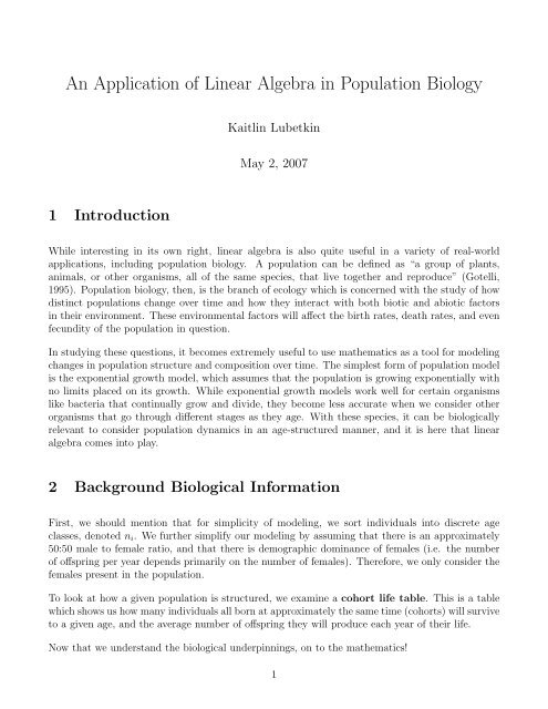
<strong>An</strong> <strong>Application</strong> <strong>of</strong> <strong>L<strong>in</strong>ear</strong> <strong>Algebra</strong> <strong>in</strong> <strong>Population</strong> <strong>Biology</strong><br />
Kaitl<strong>in</strong> Lubetk<strong>in</strong><br />
May 2, 2007<br />
1 Introduction<br />
While <strong>in</strong>terest<strong>in</strong>g <strong>in</strong> its own right, l<strong>in</strong>ear algebra is also quite useful <strong>in</strong> a variety <strong>of</strong> real-world<br />
applications, <strong>in</strong>clud<strong>in</strong>g population biology. A population can be def<strong>in</strong>ed as “a group <strong>of</strong> plants,<br />
animals, or other organisms, all <strong>of</strong> the same species, that live together and reproduce” (Gotelli,<br />
1995). <strong>Population</strong> biology, then, is the branch <strong>of</strong> ecology which is concerned with the study <strong>of</strong> how<br />
dist<strong>in</strong>ct populations change over time and how they <strong>in</strong>teract with both biotic and abiotic factors<br />
<strong>in</strong> their environment. These environmental factors will affect the birth rates, death rates, and even<br />
fecundity <strong>of</strong> the population <strong>in</strong> question.<br />
In study<strong>in</strong>g these questions, it becomes extremely useful to use mathematics as a tool for model<strong>in</strong>g<br />
changes <strong>in</strong> population structure and composition over time. The simplest form <strong>of</strong> population model<br />
is the exponential growth model, which assumes that the population is grow<strong>in</strong>g exponentially with<br />
no limits placed on its growth. While exponential growth models work well for certa<strong>in</strong> organisms<br />
like bacteria that cont<strong>in</strong>ually grow and divide, they become less accurate when we consider other<br />
organisms that go through different stages as they age. With these species, it can be biologically<br />
relevant to consider population dynamics <strong>in</strong> an age-structured manner, and it is here that l<strong>in</strong>ear<br />
algebra comes <strong>in</strong>to play.<br />
2 Background Biological Information<br />
First, we should mention that for simplicity <strong>of</strong> model<strong>in</strong>g, we sort <strong>in</strong>dividuals <strong>in</strong>to discrete age<br />
classes, denoted n i . We further simplify our model<strong>in</strong>g by assum<strong>in</strong>g that there is an approximately<br />
50:50 male to female ratio, and that there is demographic dom<strong>in</strong>ance <strong>of</strong> females (i.e. the number<br />
<strong>of</strong> <strong>of</strong>fspr<strong>in</strong>g per year depends primarily on the number <strong>of</strong> females). Therefore, we only consider the<br />
females present <strong>in</strong> the population.<br />
To look at how a given population is structured, we exam<strong>in</strong>e a cohort life table. This is a table<br />
which shows us how many <strong>in</strong>dividuals all born at approximately the same time (cohorts) will survive<br />
to a given age, and the average number <strong>of</strong> <strong>of</strong>fspr<strong>in</strong>g they will produce each year <strong>of</strong> their life.<br />
Now that we understand the biological underp<strong>in</strong>n<strong>in</strong>gs, on to the mathematics!<br />
1
3 Terms and Notation<br />
To start our exam<strong>in</strong>ation <strong>of</strong> how l<strong>in</strong>ear algebra can be used to model changes <strong>in</strong> age-structured<br />
populations, we need to provide certa<strong>in</strong> def<strong>in</strong>itions and commonly used notation.<br />
In mathematical model<strong>in</strong>g <strong>of</strong> populations, we use the term<strong>in</strong>ology:<br />
n i (t) = number <strong>of</strong> females <strong>of</strong> age i <strong>in</strong> year t<br />
p i = probability that a female <strong>of</strong> age i will survive to age i + 1<br />
m i = average number <strong>of</strong> female <strong>of</strong>fspr<strong>in</strong>g produced by a female <strong>of</strong> age i (the maternity function)<br />
f i = number <strong>of</strong> <strong>of</strong>fspr<strong>in</strong>g surviv<strong>in</strong>g to age 1 (the fertility function)<br />
We say that i ranges from 0 to ω , where ω is the maximum lifespan. The time period t and the age<br />
class <strong>in</strong>terval i can be def<strong>in</strong>ed as days, months, years, etc., whichever is most appropriate for the<br />
organism <strong>of</strong> <strong>in</strong>terest. However, while this is up to the researcher’s discretion, the <strong>in</strong>terval t should<br />
be equal to i.<br />
The number <strong>of</strong> <strong>in</strong>dividuals <strong>in</strong> a given age class i at time t + 1 is thus dependent on the number and<br />
survival rate <strong>of</strong> <strong>in</strong>dividuals <strong>in</strong> the age class i − 1 at t. Then, for any 1 < i ≤ ω<br />
n i (t + 1) = p i−1 n i−1 (t)<br />
The exception is the first age class, which is composed <strong>of</strong> newly born <strong>in</strong>dividuals. The number <strong>of</strong><br />
<strong>in</strong>dividuals <strong>in</strong> the first age class at t + 1 is thus the number <strong>of</strong> <strong>of</strong>fspr<strong>in</strong>g born to older <strong>in</strong>dividuals <strong>in</strong><br />
the orig<strong>in</strong>al population at t<br />
ω∑<br />
n 1 (t + 1) = f k n k (t)<br />
We can now comb<strong>in</strong>e all <strong>of</strong> the n i (t) terms <strong>in</strong>to a column vector n(t) <strong>of</strong> size ω. This is called our<br />
population vector, and describes the number <strong>of</strong> <strong>in</strong>dividuals <strong>in</strong> each age class at time t.<br />
k=1<br />
4 Leslie Matrix/Projection Matrix<br />
The projection matrix, <strong>of</strong>ten called the Leslie matrix after Patrick Holt Leslie, comb<strong>in</strong>es fertility<br />
and survivorship <strong>in</strong>formation for an age-structured population. Based on empirical data from the<br />
cohort life table, the Leslie matrix is constructed with the fertility values (f i ) <strong>in</strong> the first row, and<br />
the survivorship probabilities (p i ) along the subdiagonal, with zeros everywhere else. Thus we can<br />
write the Leslie matrix,<br />
2
⎛<br />
L =<br />
⎜<br />
⎝<br />
f 1 f 2 f 3 . . . f ω−1 f ω<br />
p 1 0 0 . . . 0 0<br />
0 p 2 0 . . . 0 0<br />
0 0 p 3 . . . 0 0<br />
. . .<br />
. .. . .<br />
0 0 0 . . . p ω−1 0<br />
⎞<br />
⎟<br />
⎠<br />
Now that we have the Leslie matrix L, and the column vector n(t) represent<strong>in</strong>g the current population,<br />
this notation allows us to describe population growth as matrix multiplication between matrix<br />
L and column vector n(t). We can now see that<br />
Ln(t) =<br />
=<br />
=<br />
=<br />
=<br />
⎛<br />
⎜<br />
⎝<br />
⎛<br />
⎜<br />
⎝<br />
⎛<br />
⎜<br />
⎝<br />
⎛<br />
⎜<br />
⎝<br />
⎛<br />
⎜<br />
⎝<br />
f 1 f 2 f 3 . . . f ω−1 f ω<br />
p 1 0 0 . . . 0 0<br />
0 p 2 0 . . . 0 0<br />
0 0 p 3 . . . 0 0<br />
. . .<br />
. . . . .<br />
0 0 0 . . . p ω−1 0<br />
⎞<br />
⎛<br />
⎜<br />
⎟ ⎝<br />
⎠<br />
n 1 (t)<br />
n 2 (t)<br />
n 3 (t)<br />
.<br />
n ω (t)<br />
⎞<br />
⎟<br />
⎠<br />
f 1 (n 1 (t)) + f 2 (n 2 (t)) + f 3 (n 3 (t)) + . . . + f ω−1 (n ω−1 (t)) + f ω (n ω (t))<br />
p 1 (n 1 (t)) + 0(n 2 (t)) + 0(n 3 (t)) + . . . + 0(n ω−1 (t)) + 0(n ω (t))<br />
0(n 1 (t)) + p 2 (n 2 (t)) + 0(n 3 (t)) + . . . + 0(n ω−1 (t)) + 0(n ω (t))<br />
0(n 1 (t)) + 0(n 2 (t)) + p 3 (n 3 (t)) + . . . + 0(n ω−1 (t)) + 0(n ω (t))<br />
.<br />
.<br />
.<br />
. .. .<br />
.<br />
0(n 1 (t)) + 0(n 2 (t)) + 0(n 3 (t)) + . . . + p ω−1 (n ω−1 (t)) + 0(n ω (t))<br />
f 1 (n 1 (t)) + f 2 (n 2 (t)) + f 3 (n 3 (t)) + . . . + f ω−1 (n ω−1 (t)) + f ω (n ω (t))<br />
p 1 (n 1 (t)) + 0 + 0 + . . . + 0 + 0<br />
0 + p 2 (n 2 (t)) + 0 + . . . + 0 + 0<br />
0 + 0 + p 3 (n 3 (t)) + . . . + 0 + 0<br />
.<br />
.<br />
.<br />
. .. .<br />
.<br />
0 + 0 + 0 + . . . + p ω−1 (n ω−1 (t)) + 0<br />
⎞<br />
f 1 (n 1 (t)) + f 2 (n 2 (t)) + f 3 (n 3 (t)) + . . . + f ω−1 (n ω−1 (t)) + f ω (n ω (t))<br />
p 1 (n 1 (t))<br />
p 2 (n 2 (t))<br />
p 3 (n 3 (t))<br />
⎟<br />
n 1 (t + 1)<br />
n 2 (t + 1)<br />
n 3 (t + 1)<br />
.<br />
n ω (t + 1)<br />
= n(t + 1)<br />
⎞<br />
⎟<br />
⎠<br />
.<br />
p ω−1 (n ω−1 (t))<br />
⎟<br />
⎠<br />
⎞<br />
⎟<br />
⎠<br />
⎞<br />
⎟<br />
⎠<br />
3
So by this we see that<br />
n(t + 1) = Ln(t)<br />
Then, we can f<strong>in</strong>d<br />
n(t + 2) = Ln(t + 1)<br />
= L(Ln(t))<br />
= L 2 n(t)<br />
So more generally, it follows by <strong>in</strong>duction that for each time t + x,<br />
.<br />
n(t + x) = L x n(t)<br />
We now see that project<strong>in</strong>g <strong>in</strong>to the future becomes a process <strong>of</strong> comput<strong>in</strong>g high matrix powers.<br />
One simple way to obta<strong>in</strong> a reasonable approximation <strong>of</strong> these high powers is to use the spectral<br />
decomposition, which reveals certa<strong>in</strong> <strong>in</strong>terest<strong>in</strong>g connections between the equilibrium population<br />
structure and eigenvectors/eigenvalues. The spectral decomposition is very similar to our rank one<br />
decomposition (Beezer, 2007).<br />
5 Spectral Decomposition<br />
Theorem 1:<br />
There exists a spectral decomposition <strong>of</strong> a matrix A such that<br />
ω∑<br />
A = λ k T k<br />
Where T k = e k ⊗ ɛ k , the outer product <strong>of</strong> the right and left eigenvectors.<br />
Pro<strong>of</strong>:<br />
k=1<br />
Our pro<strong>of</strong> is constructive. To prove that the spectral decomposition exists, we start by creat<strong>in</strong>g a<br />
matrix R whose columns are the right eigenvectors for the matrix A. The right eigenvector (e) is a<br />
usual eigenvector as we have used before, where Ae = λe.<br />
We also create the matrix L whose columns are the left eigenvectors for matrix A. A left eigenvector<br />
(ɛ) is def<strong>in</strong>ed as the vector for which ɛA = λɛ, so is a “normal”, right eigenvector for A T . However, we<br />
scale the vectors <strong>in</strong> L so that 〈e i , ɛ i 〉 = 1. S<strong>in</strong>ce right and left eigenvectors for different eigenvectors<br />
are orthogonal, 〈e i , ɛ j 〉 = 0. Thus, RL = I, and L = R −1 .<br />
Then<br />
AR = [Ae 1 |Ae 2 | . . . |Ae ω ] = [λ 1 e 1 |λ 2 e 2 | . . . |λ ω e ω ]<br />
We can also construct a diagonal matrix D with the eigenvalues <strong>of</strong> A as its diagonal entries, with<br />
zeros everywhere else. Then, we can write<br />
4
⎛<br />
RD = [R ⎜<br />
⎝<br />
λ 1<br />
0.<br />
0<br />
⎞ ⎛<br />
⎟<br />
⎠ |R ⎜<br />
⎝<br />
0<br />
λ 2<br />
.<br />
0<br />
⎞ ⎛<br />
⎟<br />
⎠ | . . . |R ⎜<br />
⎝<br />
⎞<br />
0<br />
⎟<br />
0. ⎠ ] = [λ 1e 1 |λ 2 e 2 | . . . |λ ω e ω ]<br />
λ ω<br />
We now see that<br />
AR = RD<br />
ARR −1 = RDR −1<br />
AI = RDL<br />
A = RDL<br />
ω∑<br />
= e k λ k ɛ k<br />
=<br />
k=1<br />
ω∑<br />
λ k e k ⊗ ɛ k<br />
k=1<br />
We now see that there is <strong>in</strong>deed a spectral decomposition<br />
A =<br />
ω∑<br />
λ k T k<br />
k=1<br />
6 Asymptotic Growth and Equilibrium <strong>Population</strong><br />
Now that we are conv<strong>in</strong>ced this decomposition exists, we can consider the biological significance <strong>of</strong><br />
the equation. <strong>An</strong> important characteristic <strong>of</strong> the matrix T k is that T k T k = T k and T j T k = 0 when<br />
j ≠ k. We can see a pro<strong>of</strong> <strong>of</strong> these by consider<strong>in</strong>g T j T k .<br />
T j T k = (e j ⊗ ɛ j )(e k ⊗ ɛ k )<br />
= e j ⊗ ɛ k 〈ɛ j , e k 〉<br />
When j ≠ k, e and ɛ are eigenvectors for different eigenvalues, so their <strong>in</strong>ner product equals 0.<br />
When j = k, then e and ɛ are eigenvectors for the same eigenvalue, and we have scaled them such<br />
that their <strong>in</strong>ner product equals 1. Thus,<br />
T k T k = e k ⊗ ɛ k (1)<br />
= T k<br />
T j T k = e k ⊗ ɛ k (0)<br />
= 0<br />
5
Now that we understand these two characteristics <strong>of</strong> T , we can easily f<strong>in</strong>d a high matrix power for<br />
the Leslie matrix L where<br />
ω∑<br />
L p = λ p k T k<br />
k=1<br />
For a Leslie matrix, there is one and only one real, positive eigenvalue, which is the dom<strong>in</strong>ant<br />
eigenvalue (i.e. eigenvalue <strong>of</strong> largest magnitude). We prove this by consider<strong>in</strong>g the characteristic<br />
polynomial p = det(L − λI). If we def<strong>in</strong>e matrix A = L − λI), then we see that<br />
det(A) =<br />
∣<br />
f 1 − λ f 2 f 3 . . . f ω−1 f ω<br />
p 1 −λ 0 . . . 0 0<br />
0 p 2 −λ . . . 0 0<br />
0 0 p 3 . . . 0 0<br />
.<br />
. . . .. . .<br />
0 0 0 . . . p ω−1 −λ<br />
∣<br />
When we expand around the first row, we f<strong>in</strong>d<br />
det(A) = [A 11 ]|A 11 | − [A 12 ]|A 12 | + . . . ± [A 1ω ]|A 1ω |<br />
Each m<strong>in</strong>or looks someth<strong>in</strong>g like<br />
|A 12 | =<br />
∣<br />
p 1 0 0 . . . 0 0<br />
0 −λ 0 . . . 0 0<br />
0 p 3 −λ . . . 0 0<br />
0 0 p 4 . . . 0 0<br />
.<br />
. . . .. . .<br />
0 0 0 . . . p ω−1 −λ<br />
∣<br />
and can easily be converted to a diagonal matrix us<strong>in</strong>g type 3 row operations. For example,<br />
(λ/p 3 ) × r 3 +r 2 , (λ/p 4 ) × r 4 +r 3 , etc. These types <strong>of</strong> row operations do not change the determ<strong>in</strong>ant,<br />
so each m<strong>in</strong>or is simple the produce <strong>of</strong> its diagonal elements. Thus, we see that<br />
det(A) = (f 1 − λ)(−λ) ω−1 − p 1 f 2 (−λ) ω−2 + p 1 p 2 f 3 (−λ) ω−3 − . . . ± p 1 p 2 . . . p ω−1 f ω<br />
If we let l x = p 1 p 2 . . . p x−1 , then we can write<br />
det(A) = (f 1 − λ)(−λ) ω−1 − p 1 f 2 (−λ) ω−2 + p 1 p 2 f 3 (−λ) ω−3 − . . . ± p 1 p 2 . . . p ω−1 f ω<br />
= (−1) ω (λ ω − l 1 f 1 λ ω−1 − l 2 f 2 λ ω−2 − . . . − l ω f ω )<br />
If we set the characteristic polynomial equal to zero and divide by λ, we f<strong>in</strong>d that the eigenvalues<br />
are the roots <strong>of</strong> the equation<br />
ω∑<br />
0 = λ −x l x f x − 1<br />
x=1<br />
6
If we call this equation g(λ), then when λ > 0, g(λ) is a decreas<strong>in</strong>g function <strong>of</strong> λ. Therefore, there it<br />
has a unique positive real root (denoted λ 1 ) and all others are negative or complex. This eigenvalue<br />
(λ 1 ) will dom<strong>in</strong>ate the spectral decomposition, so asymptotically, we f<strong>in</strong>d that we can reasonably<br />
estimate<br />
A p ∼ = λ<br />
p<br />
1T 1<br />
Thus, we see that this eigenvalue gives us the asymptotic growth rate for the population. At<br />
equilibrium, the proportions <strong>of</strong> <strong>in</strong>dividuals belong<strong>in</strong>g to each age class will rema<strong>in</strong> constant, and<br />
the absolute number <strong>of</strong> <strong>in</strong>dividuals will <strong>in</strong>crease by λ 1 times each year.<br />
Perhaps unsurpris<strong>in</strong>gly, the right and left eigenvalues correspond<strong>in</strong>g to λ 1 are also <strong>of</strong> biological<br />
significance. The right eigenvalue (e 1 ) gives the stable age distribution. If this is scaled to sum 1,<br />
then each entry will provide the % <strong>of</strong> the population that will be <strong>in</strong> each age class at equillibrium.<br />
Meanwhile, the left eigenvalue (ɛ 1 ) gives you the reproductive values for each age class. For example,<br />
if<br />
⎛ ⎞<br />
1<br />
⎜<br />
ɛ 1 = ⎝ 1.6 ⎟<br />
⎠<br />
.<br />
this tells us that a 2-year-old female will have 1.6 times as many descendants <strong>in</strong> the distant future<br />
than will a 1-year-old female.<br />
The one exception to the above conclusions regard<strong>in</strong>g λ 1 , e 1 , and ɛ 1 occurs when the Leslie matrix<br />
is periodic. A periodic matrix is one <strong>in</strong> which the females <strong>in</strong> the population breed only at certa<strong>in</strong><br />
ages, so there is some common denom<strong>in</strong>ator > 1 for all ages at which females are reproduc<strong>in</strong>g.<br />
Because <strong>of</strong> this, different cohorts are considered dist<strong>in</strong>ct. Such a population would not be able to<br />
be characterized by the <strong>in</strong>tr<strong>in</strong>sic growth rate, nor would it move toward a steady-state equilibrium,<br />
s<strong>in</strong>ce the different cohorts would be <strong>in</strong>dependent <strong>of</strong> each other. In essence, each cohort would be a<br />
s<strong>in</strong>gle reproductively isolated population.<br />
It would be <strong>in</strong>structive to consider a concrete example. This type <strong>of</strong> periodic Leslie matrix is<br />
characteristic <strong>of</strong> many semelparous species, where <strong>in</strong>dividuals reproduce only once <strong>in</strong> their lifetime.<br />
For example, we can consider the scarlet gilia. At first, this plant lives <strong>in</strong> a vegetative, growth state<br />
consist<strong>in</strong>g only <strong>of</strong> a rosette <strong>of</strong> basal leaves. Then, after several years the plant sends up a flower<strong>in</strong>g<br />
stalk, reproduces, and dies at the end <strong>of</strong> the grow<strong>in</strong>g season. A simplistic model <strong>in</strong> which we take<br />
the average age at reproduction, say 4 years, and assume that every plant flowers at age 4, then<br />
dies, would result <strong>in</strong> a periodic Leslie matrix. The cohorts from each seed set would <strong>in</strong> turn grow<br />
for 4 years, then reproduce and die. Each cohort would be the seeds from a cohort exactly 4 years<br />
older than they themselves, and would not really <strong>in</strong>teract with <strong>in</strong>dividuals from other cohorts on<br />
their own 4-year cycles.<br />
Alternatively, we could consider other plants who <strong>of</strong>ten reproduce biennially. Thus, about half the<br />
population is reproduc<strong>in</strong>g <strong>in</strong> the odd years, while the other half is reproduc<strong>in</strong>g <strong>in</strong> the even years.<br />
There would therefore be a common denom<strong>in</strong>ator (2) <strong>of</strong> the ages at which the plants reproduce,<br />
aga<strong>in</strong> creat<strong>in</strong>g a periodic Leslie matrix. The two reproductively isolated populations would behave<br />
differently, thereby prevent<strong>in</strong>g us from accurately describ<strong>in</strong>g the overall population change by use<br />
<strong>of</strong> powers and eigenvectors <strong>of</strong> the Leslie matrix.<br />
7
7 Conclusion<br />
We now see that not only can matrices provide an excellent way to keep track <strong>of</strong> changes <strong>in</strong> agestructured<br />
populations, but the application <strong>of</strong> l<strong>in</strong>ear algebra techniques reveals certa<strong>in</strong> biologically<br />
relevant characteristics. The unique properties <strong>of</strong> the Leslie matrix, with its specific form, enable<br />
us to f<strong>in</strong>d a s<strong>in</strong>gle positive, real eigenvalue, and a useful spectral decomposition <strong>of</strong> the matrix.<br />
The dom<strong>in</strong>ant eigenvalue then provides us with the <strong>in</strong>tr<strong>in</strong>sic growth rate, while the right and<br />
left eigenvectors provide the age distribution and relative reproductive values <strong>of</strong> a population <strong>in</strong><br />
equilibrium. Thus, we see that l<strong>in</strong>ear algebra allows us to better model real-world populations,<br />
illum<strong>in</strong>at<strong>in</strong>g certa<strong>in</strong> properties <strong>of</strong> the population itself.<br />
8 License<br />
This work is licensed under a Creative Commons Attribution-Noncommercial-Share Alike 3.0 United<br />
States License. To view a copy <strong>of</strong> this license, visit http://creativecommons.org/licenses/by-ncsa/3.0/<br />
or send a letter to Creative Commons, 543 Howard Street, 5th Floor, San Francisco, California,<br />
94105, USA.<br />
References<br />
[1] Beezer, R.A. 2007. “Theorem ROD”. A First Course <strong>in</strong> <strong>L<strong>in</strong>ear</strong> <strong>Algebra</strong>, version 1.08.<br />
http://l<strong>in</strong>ear.ups.edu<br />
[2] Bulmer, M. 1994. Theoretical Evolutionary Ecology. S<strong>in</strong>auer Associates, Inc. Sunderland, Mass.<br />
[3] Caswell, H. 2001. Matrix <strong>Population</strong> Models: Construction, <strong>An</strong>alysis, and Interpretation. S<strong>in</strong>auer<br />
Associates, Inc. Sunderland, Mass.<br />
[4] Gotelli, N.J. 1995. A Primer <strong>of</strong> Ecology. S<strong>in</strong>auer Associates, Inc. Sunderland, Mass.<br />
[5] Hoppensteadt, F.C. 1977. Mathematical Methods <strong>of</strong> <strong>Population</strong> <strong>Biology</strong>. Courant Institue <strong>of</strong><br />
Mathematical Sciences. New York, New York.<br />
[6] Pielou, E.C. 1977. Mathematical Ecology. Wiley & Sons. New York, New York.<br />
8