An Interim Channel Model for Beyond-3G Systems - Giovanni Del ...

An Interim Channel Model for Beyond-3G Systems
Extending the 3GPP Spatial Channel Model (SCM)
Daniel S. Baum and Jan Hansen
Communication Technology Laboratory
ETH Zürich, Switzerland
dsbaum@nari.ee.ethz.ch
Jari Salo
Radio laboratory/SMARAD
Helsinki University of Technology, Espoo, Finland
jari.salo@hut.fi
Giovanni Del Galdo and Marko Milojevic
Fachgebiet Nachrichtentechnik
Technische Universität Ilmenau, Ilmenau, Germany
{giovanni.delgaldo,marko.milojevic}@tu-ilmenau.de
Pekka Kyösti
Elektrobit
Oulu, Finland
pekka.kyosti@elektrobit.com
Abstract— This paper reports on the interim beyond-3G channel
model developed by and used within the European WINNER
project. The model is a comprehensive spatial channel model for
2 and 5 GHz frequency bands and supports bandwidths up to 100
MHz in three different outdoor environments. It further features
a time-variable system-level parameters for challenging advanced
communication algorithms, as well as a reduced variability
tapped delay-line model for improved usability in calibration and
comparison simulations.
Keywords-beyond-3G, channel model, MIMO, SCM, 3GPP
I. INTRODUCTION
In recent years Multiple-Input Multiple-Output (MIMO)
wireless communication techniques have attracted strong
attention in research and development due to their potential
benefits in spectral efficiency, throughput and quality of
service. Only recently, however, has this technology been
considered to be included in wireless communication system
standards, such as IEEE 802.11n for wireless LANs (WLAN),
IEEE 802.16 for broadband fixed wireless access (FWA), and
3GPP HSDPA for cellular mobile communications.
Any wireless communication system needs to specify a
propagation channel model that can act as a basis for performance
evaluation and comparison. With advancing communication
technologies, these models need to be refined as
further characteristics of the channel can be exploited and thus
need to be modeled. To enable MIMO, the standardization
groups 802.11 and 3GPP thus first defined spatial channel
models suitable for their applications [1], [2].
Upcoming communication systems will be based on new
range of system parameters (e.g., extended bandwidth and new
frequency bands), a broader range of and additional scenarios
(e.g., mobile to mobile, mobile hotspot), and new
communication techniques (e.g., tracking algorithms). This
triggers new requirements on the underlying channel models.
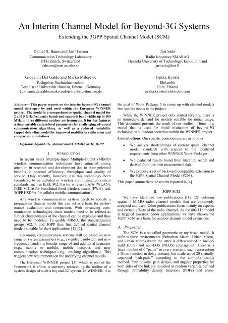
The European WINNER project [3], which is part of the
Framework 6 effort, is currently researching the outline of a
system design of such a beyond-3G system. In WINNER, it is
the goal of Work Package 5 to come up with channel models
that suit the needs in the project.
While the WINNER project only started recently, there is
an immediate demand for models suitable for initial usage.
This document presents the result of our studies in form of a
model that is used for initial evaluation of beyond-3G
technologies in outdoor scenarios within the WINNER project.
Contributions. Our specific contributions are as follows:
• We analyze shortcomings of current spatial channel
model standards with respect to the identified
requirements from other WINNER Work Packages.
• We evaluated results found from literature search and
derived from our own measurement data.
• We propose a set of backward compatible extension to
the 3GPP Spatial Channel Model (SCM).
This paper summarizes the results reported in [4].
II.
3GPP SCM
We have identified two publications ([1], [2]) defining
spatial / MIMO radio channel models that are commonly
accepted and used. Other publications focus mainly on aspects
and certain effects of the radio channel. As the 802.11n model
is targeted towards indoor applications, we have chosen the
3GPP SCM as a basis for outdoor channel model extensions.
A. Properties
The SCM is a so-called geometric or ray-based model. It
defines three environments (Suburban Macro, Urban Macro,
and Urban Micro) where the latter is differentiated in line-ofsight
(LOS) and non-LOS (NLOS) propagation. There is a
fixed number of 6 “paths” in every scenario, each representing
a Dirac function in delay domain, but made up of 20 spatially
separated “sub-paths” according to the sum-of-sinusoids
method. Path powers, path delays, and angular properties for
both sides of the link are modeled as random variables defined
through probability density functions (PDFs) and cross-

Scenario
correlations. All parameters, except for fast-fading, are drawn
independently in time, in what is termed “drops”.
B. Shortcomings
The SCM was defined for a 5 MHz bandwidth CDMA
system in the 2 GHz band, whereas the currently defined
WINNER system parameters are 100 MHz in both 2 and 5
GHz frequency range. Other minor issues are the drop based
concept, i.e., no short-term system-level time-variability in the
model, the lack of Ricean K-factor models (LOS support) for
macro scenarios, and the lack of a rural scenario.
III.
TABLE 1. MIDPATH POWER-DELAY PARAMETERS
Suburban Macro,
Urban Macro
Urban Micro
No. mid-paths per path 3 4
Mid-path power and
delay relative to
paths (ns)
1 10/20 0 6/20 0
2 6/20 7 6/20 5.8
3 4/20 26.5 4/20 13.5
4 - - 4/20 27.6
INTERIM BEYOND-3G CHANNEL MODEL
Our main goal for the extension was to keep it simple,
straightforward, and backward-compatible. This approach
provides consistency and comparability. In the following we
discuss the underlying concepts and the reasoning behind the
proposed extensions.
A. Bandwidth
To extend the model in a way such that its characteristics
remain unchanged if compared at the original 5 MHz
resolution bandwidth, we add intra-path delay-spread (DS),
which is zero in the SCM. A possible power-delay profile
(PDP) is a one-sided exponential function. This approach of
intra-cluster delay-spread was originally proposed by Saleh and
Valenzuela for indoor propagation modeling [7]. It has also
been adopted as the intra-cluster delay-spread model for
outdoor scenarios in the COST259 [8] model. Following the
SCM philosophy, which is based on COST259, we use this as
our guideline.
The path DS was chosen under the following considerations
• Similar to the definition of a constant path AS for a
specific scenario in SCM, we set the path DS to be
constant. The path AS and DS then define the
minimum observable total (over all paths) AS and DS.
• Both from measurements and intuition it follows that
this minimum total spread lies somewhere between
zero and a fraction of the mean total spread.
• The error in power between an exponential PDP and
the SCM definition (no DS) is illustrated in Figure 1.
For a path DS of 10 ns, this error is slightly below -20
dB and can be considered reasonably small. We set it
equivalent to this value for all paths.
We split the 20 sub-paths into subsets, denoted “midpaths”,
which we then move to different delays relative to the
original path. Even though a mid-path consists of multiple subpaths,
it remains a single tap (delay-resolvable component).
This approach limits the diversity increase to reasonable
values, and avoids that single sub-paths become delayresolvable.
Furthermore, lumping together a number of subpaths
keeps the fading distribution of that tap close to Rayleigh
and thus aids a potential implementation with the classic
Gaussian-distributed number generator. We found that 4 is the
absolute minimum number of sinusoids to yield a reasonable
Rayleigh distribution.
The number of mid-paths, and the power and delay
parameters chosen for each mid-path are tabulated in Table 1.
The mid-path powers, i.e. number of sub-paths, were chosen by
considering the decreasing power with delay while staying
above the minimum number of sub-paths. The delays for the
mid-paths were then derived by employing the method from
[5] and using the constraint that the DS is equal to the
predetermined value of 10 ns and given the predetermined set
of powers for the mid-paths.
Each sub-path has an angle relative to the path mean angle
assigned to it. By perturbing the set of sub-paths assigned to a
mid-path, the AS of that mid-path can be varied. It has been
reported, e.g. [6], that the intra-cluster AS conditioned on the
intra-cluster delay is approximately independent of the delay.
Hence, the mid-path ASs (AS m ) were optimized such that the
deviation from the path AS (AS p ), i.e. the AS of all mid-paths
combined, is minimized. The result is tabulated in Table 3.
Finally, to aid in channel model implementation, we
quantize the delay values to multiples of 1 ns.
B. Frequency Range
1) Path-Loss Model
The SCM path-loss model is based on the COST-Hata-
Model [10] for Suburban and Urban Macro scenarios. The
COST-Walfish-Ikegami-Model (COST-WI) [10] is defined for
error power below original signal in dB
0
-5
-10
-15
-20
-25
-30
-35
-40
-45
3 mid-paths
4 mid-paths
10 0 10 1
delay-spread in ns
Figure 1. Relative power of channel impulse response difference when path-
DS is added, compared at 5 MHz bandwidth

TABLE 3. SUB-PATHS TO MID-PATHS ASSIGNMENT AND RESULTING
NORMALIZED MID-PATH ANGLE-SPREADS
Midpath
3 mid-path configuration 4 mid-path configuration
Pwr Sub-paths AS m /
AS p
Pwr Subpaths
AS m /
AS p
1 10/20 1, 2, 3, 4, 5,
6, 7, 8, 19, 20
2 6/20 9, 10, 11, 12,
17, 18
Urban Micro. Some further references on path loss were found
([11]-[18]), however only few of them allow direct comparison
between equivalent measurements at 2 and 5 GHz. These few
however indicate that the most significant difference can be
attributed to different gains in free-space path-loss, which is 8
dB higher at 5 GHz compared to 2 GHz. Thus, for
comparability reasons, we propose a 5 GHz path-loss model
that has an offset of 8 dB to the current 2 GHz model.
There are some issues here though. The COST-231-Hata-
Model was derived for the purpose of GSM coverage
prediction and has a distance range of 1-20 km. The 5 GHz
band on the other hand is likely going to be used for shortrange
high-throughput services. In this case, a path-loss based
on the COST-WI model with a distance range of 0.02-5 km is
much more suitable. Note that this model has also been
accepted by the ITU-R and was selected as Urban / Alternative
Flat Suburban path-loss model in the IEEE 802.16 standard for
fixed wireless access [19]. Furthermore, the model
distinguishes between LOS and NLOS situations.
We propose to use the COST-WI model for all scenarios
with the following parameters: base station (BS) antenna
height: 32 m – Macro, 10 m – Micro; building height: 12 m –
Urban, 9 m – Suburban; building to building distance: 50 m,
street width: 25 m, mobile station (MS) antenna height: 1.5 m,
orientation: 30° for all paths, and selection of medium sized
city / suburban centres – Macro, metropolitan - Micro. The
Scenario
TABLE 2. PATH-LOSS MODEL
Suburban
Macro
31.5 +
35.0 log 10(d)
Urban
Macro
34.5 +
35.0 log 10(d)
SCM pathloss
NLOS
(dB),
d is in m LOS - -
Urban
Micro
34.53 +
38.0 log 10(d)
30.18 +
26.0 log 10(d)
SCM shad. NLOS 8 8 10
std. dev. (dB) LOS - - 8
Alternative.
short-range
path-loss
Alt. shad. std.
Dev. (dB)
5 GHz PL
ext.
NLOS
LOS
7.17 +
38.0 log 10(d)
30.18 +
26.0 log 10(d)
0.9865 6/20 1, 2, 3,
4, 19, 20
1.0056 6/20 5, 6, 7,
8, 17, 18
3 4/20 13, 14, 15, 16 1.0247 4/20 9, 10,
15, 16
4 - - - 4/20 11, 12,
13, 14
11.14 +
38.0 log 10(d)
30.18 +
26.0 log 10(d)
31.81 +
40.5 log 10(d)
30.18 +
26.0 log 10(d)
(N)LOS 8 8 8
1.2471
0.9145
0.8891
0.7887
(N)LOS + 8 dB + 8 dB + 8 dB
results are summarized in Table 2.
2) Delay-Spread, Angle-Spread and Ricean K-factor
A preliminary measurement analysis indicates that for
Urban Micro the 5 GHz PDP and PAS do not significantly
deviate from the 2 GHz one and we thus leave it unchanged.
However, there is evidence that in urban macro and suburban
macro there is noticeable difference in the decay rates of the 2
GHz and 5 GHz PDP. Therefore, for these environments, we
propose rms delay spread values based on 5 GHz measurement
analysis.
Similarly, we propose using the 2 GHz K-factor for 5 GHz
range. More energy escapes in reflections at 5 GHz but also the
direct path is more attenuated, so the effects cancel out in a first
order approximation. We apply the same argument in the case
of shadowing and make no differentiation for frequency range.
C. Other Extensions
1) LOS for All Scenarios
In the SCM, the LOS model consisting of path-loss and
Ricean K-factor definition is a switch selectable option for the
Urban Micro scenario only. We extend the K-factor option to
cover also Urban and Suburban Macro scenarios as follows.
Urban and Suburban Macro are assigned the same
parameters. The probability of having LOS is calculated as [20]
⎛ h ⎞⎛ ⎞
= ⎜ −
B d
P ⎟
⎜ −
⎟
LOS
1 1 , d
co
< 300 , h
BS
> hB
⎝ hBS
⎠⎝
d
co ⎠
and is zero otherwise. Here, h BS is the BS height, h B the average
height of the rooftops, and d co is the cut-off distance. Values for
these parameters are proposed in [8].
We use the empirical K-factor model presented in [21] for
typical (American) suburban environments and BS heights of
approximately 20 m. In [22], an excellent agreement with this
model was reported based on independent measurements under
similar conditions. We propose the following parameters: MS
antenna height 1.5 m, MS beamwidth: 360°, and selection of
season: summer. The resulting model is
K = 15.4
− 5.0 ⋅ log10 ( d ) (dB)
where d is the BS-MS distance in m.
2) Time-Evolution
The literature on dynamic channel models, that is, channel
models with time-varying parameters, is relatively scarce.
Initial references dynamic channel models appear to be [24],
[25], [26]. Dynamic channel models for indoor environments
are developed in [27], [28], [29], of which the first reference
focuses on dynamic delay domain characterization and the
latter two also incorporate spatial dynamics of the indoor
channel. The standard [30] defines a simple model for varying
tap delays and tap birth-death. However, this model is intended
for receiver testing and does not represent a realistic channel.
Analytical tools for characterization of non-stationary radio
channel have been presented in [31].

The concept of drops in SCM can be seen as relatively
short channel observation periods that are significantly
separated from each other in time or space such that systemlevel
parameters become constant and independent during
these periods. Our approach is to virtually extend the lengths of
these periods by adding short-term time-variability of some
system-level parameters within the drops. All parameters
remain independent between drops. The three effects we model
are discussed in the following.
a) Drifting of Tap Delays
Based on the geometric modeling and the propagation
parameters, the delay drift ( ∆ τ) of a tap delay (τ) can be
calculated directly from the velocity of MS (v), direction of MS
movement (θ v ), the AoA (θ AoA ), and sample density per
wavelength (D S ), where the angles are defined with respect to
the normal of antenna broadside.
The time between two consecutive samples (not drops) and
the distance moved by the MS during this time is
∆
λ
t =
2vD S
and λ
l = , respectively.
2
D S
The change in tap-delay between two consecutive samples
can be derived as
∆
τ
l
= cos(θ) , where θ = θ v
−θ
AoA
c
and c is the speed of light.
b) Drifting of Angles of Arrival
In the case of AoA, the drift can be geometrically
calculated as well, but one of the parameters is the distance
between MS and last-bounce scatter, and this is unknown.
SCM is not a single-bounce geometrical model and thus there
is only a weak statistical dependence between AoAs and AoDs.
Hence the unknown distance cannot simply be inferred from
the geometry, and instead we propose a stochastic model where
the distance is a random variable. As an initial model for the
PDF, we selected a log-normal distribution with a constant,
small offset and parameters according to Table 4.
In general, the angle θ is a function of time. For BS-MS
distances above 10 m, a linearization of this function yields a
very good approximation for observation periods over
hundreds of meters. If θ is linear in time, the rate of change ∆ θ
is constant and can be derived as
∆
θ = ∆
θ 0
for d
n
< d
n
∆
where
d
⎛ d ⎞
n
sin( θ
n
)
θ =
⎜
⎟
0
arcsin
⎝ d
n+
1 ⎠
=
d
+ s
θ = 180−
θ otherwise,
,
+1 ∆
∆ 0
− 2d
l cos( θ
2 2
n+
1 n
n n
and n is the sample-time index.
c) Drifting of Shadow Fading
)
TABLE 4. DISTRIBUTION PARAMETERS FOR d 0
= d min
+ X AND
CORRELATION DISTANCES FOR SHADOW FADING
Scenario
Suburban Macro 10
Urban Macro 10
d min
Parameters of log(X)
(m) mean var.
The time-evolution of shadow fading is determined by its
spatial autocorrelation function. References show that an
exponential function fits well and the drifting can thus be
modeled by a first order autoregressive process.
Derived from publications on measurement data around 2
GHz ([32]-[38]), we propose using correlation distances (50%
correlation point) listed in Table 4.
3) Tapped Delay-Line Model
In the SCM specification most parameters are defined by
their PDFs. While this provides richness in variability, it can
turn out to be a headache for accurate simulations where the
simulation time grows exponentially with the number of
random parameters. As a practical add-on we have thus defined
a set of fixed values for the power, delays, and angles of cluster
and intra-cluster taps. This is similar to the SCM link-level
model. However, while this model targets 3GPP comparability,
our solution is close to the system-level model and furthermore
optimized for small frequency autocorrelation.
The fixed delays of the 6 paths defined in SCM were fitted
to the PDP of the SCM system-level model using the method
from [5]. These delays were then perturbed until a satisfactory
frequency decorrelation was achieved.
IV.
τ
2 + 2
τ
τ
2 + 2
τ
−τ
−τ
IMPLEMENTATION
The original SCM has been implemented in MATLAB 1 and
is available [23] under a public license. Please check the
referenced website for updated information about any
extensions of the implementation.
REFERENCES
[1] V. Erceg, L. Schumacher, P. Kyritsi, A. Molisch, D. S. Baum, A. Y.
Gorokhov et al., “TGn Channel Models”, IEEE 802.11-03/940r2, Jan.
2004.
[2] 3GPP TR 25.996, “3rd Generation Partnership Project; technical
specification group radio access network; spatial channel model for
MIMO simulations (release 6)”, V6.1.0.
[3] 6 th Framework Programme, Information Society Technologies, Wireless
World Initiative New Radio (WINNER), IST-2003-507591, [online]
https://www.ist-winner.org/
[4] D. S. Baum, G. Del Galdo, J. Salo, P. Kyösti, T. Rautiainen, M.
Milojevic, and J.Hansen, “SCM Extensions,” WINNER WP5.5, Jan.
2005.
1 MATLAB is a registered trademark of The MathWorks, Inc.
1
50%
correlation
point (m)
n 1
1 200
P
−τ
−τ
n 1
1 50
Urban Micro 10 2 1 5
P
1

TABLE 5. TAPPED DELAY-LINE PARAMETERS
Scenario Suburban Macro Urban Macro Urban Micro
Power-delay parameters:
relative path power (dB) /
delay (µs)
1 0 0 0 0 0 0
2 -2.6682 0.1408 -2.2204 0.3600 -1.2661 0.2840
3 -6.2147 0.0626 -1.7184 0.2527 -2.7201 0.2047
4 -10.4132 0.4015 -5.1896 1.0387 -4.2973 0.6623
5 -16.4735 1.3820 -9.0516 2.7300 -6.0140 0.8066
6 -22.1898 2.8280 -12.5013 4.5977 -8.4306 0.9227
Resulting total DS (µs) 0.231 0.841 0.294
Path AS at BS, MS (deg) 2, 35 2, 35 5, 35
Angular parameters:
AoA (deg) /
AoD (deg)
1 156.1507 -101.3376 65.7489 81.9720 76.4750 -127.2788 0.6966 6.6100
2 -137.2020 -100.8629 45.6454 80.5354 -11.8704 -129.9678 -13.2268 14.1360
3 39.3383 -110.9587 143.1863 79.6210 -14.5707 -136.8071 146.0669 50.8297
4 115.1626 -112.9888 32.5131 98.6319 17.7089 -96.2155 -30.5485 38.3972
5 91.1897 -115.5088 -91.0551 102.1308 167.6567 -159.5999 -11.4412 6.6690
6 4.6769 -118.0681 -19.1657 107.0643 139.0774 173.1860 -1.0587 40.2849
Resulting total AS at BS,MS (deg) 4.70, 64.78 7.87, 62.35 15.76, 62.19 18.21, 67.80
[5] J. Kivinen et al, “Empirical characterization of wideband indoor radio
channel at 5.3 GHz,” IEEE Tr. Ant. Prog., pp. 1192-1203, Aug 2001.
[6] K. I. Pedersen, P. E. Mogensen, and B. H. Fleury, “A stochastic model
of the temporal and azimuthal dispersion seen at the base station in
outdoor propagation environments,” IEEE Trans. Veh. Technol., vol. 49,
no. 2, Mar. 2000, pp. 437-447.
[7] A. Saleh, and R. A. Valenzuela, “A statistical model for indoor
multipath propagation,” IEEE J. Select. Areas Commun., vol. SAC-5,
no. 2, pp. 128-137, Feb. 1987.
[8] L. M. Correia, Wireless Flexible Personalized Communications, COST
259: European Cooperation in Mobile Radio Research, Chichester: John
Wiley & Sons, 2001. Section 3.2 by M. Steinbauer and A. F. Molisch,
“Directional channel models”.
[9] J. Meinilä, T. Jämsä, P. Kyösti, D. Laselva, H. El-Sallabi, J. Salo, C.
Schneider, and D. S. Baum, “Determination of Propagation Scenarios,”
WINNER D5.2, Jun. 2004.
[10] COST 231, “Urban transmission loss models for mobile radio in the
900- and 1800 MHz bands (Revision 2),” COST 231 TD(90)119 Rev. 2,
The Hague, The Netherlands, Sep. 1991.
[11] V. Erceg, K. V. S. Hari, M. S. Smith, D. S. Baum, P. Soma, L. J.
Greenstein et al., “Channel models for fixed wireless applications,”
IEEE 802.16a-03/01, Jun. 2003.
[12] A. J. Rustako, Jr., V. Erceg, R. S. Roman, T. M. Willis, and J. Ling,
“Measurements of microcellular propagation loss at 6 GHz and 2 GHz
over NLOS paths in the city of Boston,” in Proc. IEEE
GLOBECOM’95, vol. 1, Nov. 1995, pp. 758–763.
[13] A. Karlsson, R. E. Schuh, C. Bergljung, P. Karlsson, and N. Lowendahl,
“The influence of trees on radio channels at frequencies of 3 and 5
GHz,” in Proc. IEEE VTC’01, vol. 4, Oct. 2001, pp. 2008–2012.
[14] N. Kita, A. Sato, and M. Umehira, “A path loss model with height
variation in residential area based on experimental and theoretical
studies using a 5G/2G dual band antenna,” in Proc. IEEE VTC’00, vol.
2, Sep. 2000, pp. 840–844.
[15] X. Zhao, J. Kivinen, and P. V. K. Skog, “Propagation characteristics for
wideband outdoor mobile communications at 5.3 GHz,” IEEE J. Select.
Areas Commun., vol. 20, Apr. 2002, pp. 507–514.
[16] K. Yonezawa, T. Maeyama, H. Iwai, and H. Harada, “Path loss
measurement in 5 GHz macro cellular systems and consideration of
extending existing path loss prediction methods,” in Proc. IEEE
WCNC’04, vol. 1, Mar. 2004, pp. 279–283.
[17] C.-C. Chong, C.-M. Tan, D. I. Laurenson, S. McLaughlin, M. A. Beach,
and A. R. Nix, “A new statistical wideband spatio-temporal channel
model for 5 GHz band WLAN systems,” IEEE J. Select. Areas
Commun., vol. 21, no. 2, Feb. 2003.
[18] X. Zhao, T. Rautiainen, K. Kalliola, and P. Veinikainen, “Path Loss
Models for Urban Microcells at 5.3 GHz,” COST 273 TD(04)207,
Duisburg, Germany, Sep. 2004.
[19] V. Erceg, K. V. S. Hari, M. S. Smith, D. S. Baum, et al., “Channel
models for fixed wireless applications,” IEEE Broadband Wireless
Access Working Group, Tech. Rep., IEEE 802.16.3c-01/29r4, Jul. 2001.
[20] H. Asplund and J.-E. Berg, Leidschendam, The Netherlands, Tech. Rep.
COST 259 TD(99)108, Sep. 1999.
[21] L.J.Greenstein, S.Ghassemzadeh, V.Erceg, and D.G.Michelson, “Ricean
K-Factors in Narrowband Fixed Wireless Channels,” in Proc.
WPMC’99, Amsterdam, The Netherlands, Sep. 1999.
[22] P. Soma, D. S. Baum, V. Erceg, R. Krishnamoorthy, and A. J. Paulraj,
“Analysis and modeling of multiple-input multiple-output (MIMO) radio
channel based on outdoor measurements conducted at 2.5 GHz for fixed
BWA applications,” May 2002.
[23] J. Salo, G. Del Galdo, J. Salmi, P. Kyösti, M. Milojevic, D. Laselva, and
C. Schneider. (2005, Jan.) MATLAB implementation of the 3GPP
Spatial Channel Model (3GPP TR 25.996) [Online]. Available:
http://www.tkk.fi/Units/Radio/scm/
[24] S. Papantoniou, “Modelling the mobile radio channel,” Ph.D.
dissertation, ETHZ, 1990.
[25] R. Heddergott, U. Bernhard, and B. Fleury, “Stochastic radio channel
model for advanced indoor mobile communications systems,” in Proc.
8th IEEE Int. Symp. on Personal, Indoor and Mobile Radio
Communications (PIMRC ’97), Helsinki, Finland, 1997, pp. 140–144.
[26] B. Fleury and U. B. R. Heddergott, “Advanced radio channel model for
Magic WAND,” in Proc. ACTS Mobile Summit, Granada, Spain, 1996,
pp. 600–607.
[27] J. Ødum Nielsen, V. Afanassiev, and J. B. Andersen, “A dynamic model
of the indoor channel,” Wireless Personal Communications, vol. 19, pp.
91–120, 2001.
[28] T. Zwick, C. Fischer, and W. Wiesbeck, “A stochastic multipath channel
model including path directions for indoor environments,” IEEE J.
Select. Areas Commun., vol. 20, no. 6, pp. 1178–1192, Aug. 2002.
[29] C.-C. Chong, D. I. Laurenson, and S. McLaughlin, “The implementation
and evaluation of a novel wideband dynamic directional indoor channel
model based on a Markov process,” in Proc. IEEE PIMRC, vol. 1, 2003,
pp. 670–674.
[30] “3GPP TS 25.104, v6.7.0,” Sep. 2004. [Online]. Available:
www.3gpp.org
[31] G. Matz, “Characterization of non-WSSUS fading dispersive channels,”
in Proc. IEEE Intern. Conf. Comm., vol. 4, 2003, pp. 2480–2484.
[32] M. Marsan, G. Hess, and S. Gilbert, “Shadowing variability in an urban
land mobile environment at 900 MHz,” El. Lett., vol. 26, no. 10, pp.
646–648, May 1990.

[33] E. Perahia, D. Cox, and S. Ho, “Shadow fading cross-correlation
between base stations,” in Proc. IEEE Veh. Tech. Conf. (spring), 2001.
[34] A. Algans, K. Pedersen, and P. Mogensen, “Experimental analysis of
joint statistical properties of azimuth spread, delay spread, and shadow
fading,” IEEE J. Select. Areas Commun., vol. 20, no. 3, Apr. 2002.
[35] M. Gudmundson, “Correlation model for shadow fading in mobile radio
systems,” El. Lett., vol. 27, no. 23, pp. 2145–2146, Nov. 1991.
[36] J. Weitzen and T. J. Lowe, “Measurement of angular and distance
correlation properties of log-normal shadowing at 1900 MHz and its
application to design of PCS systems,” IEEE Trans. Veh. Technol., vol.
51, no. 2, pp. 265–273, Mar. 2002.
[37] T. Sørensen, “Correlation model for slow fading in a small urban macro
cell,” in Proc. IEEE PIMRC, 1998.
[38] J. Berg, R. Bownds, and F. Lotse, “Path loss and fading models for
microcells at 900 MHz,” in Proc. IEEE Veh. Tech. Conf. (spring), 1992.