The Time-Resolved Fluorescence Techniques - Photon Technology ...

The Time-Resolved Fluorescence Techniques
There are three common techniques used in time-resolved fluorescence spectroscopy: the stroboscopic
technique (strobe), the time-correlated single photon counting technique (TCSPC) and the frequency
modulation or phase shift technique (phase). The first two are time-domain techniques while the last one is a
frequency-domain technique.
The time-domain techniques, i.e. the strobe and TCSPC, are very similar in what they measure and in the way
data are analyzed. The differences are mainly in the hardware, they use different detection electronics and
different pulsed light sources, although some light sources can be used with both techniques.
The time-domain techniques are direct techniques. They measure fluorescence decay curves (i.e. fluorescence
intensity as a function of time) directly and the experimenter has full advantage of seeing the physical
mechanism in the course of the experiment. Frequently, a qualitative judgement about a particular mechanism
can be made by examining raw decay data and a proper fitting function can be thus selected.
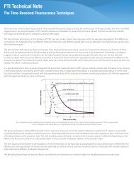
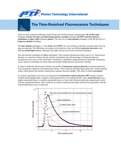
In order to obtain the fluorescence lifetime, the profile of instrument response function (excitation pulse) has
to be measured in addition to the fluorescence decay. This is because the lamp (laser) pulse has a finite temporal
width, which distorts the intrinsic fluorescence response from the sample. This effect is called convolution.
In a typical experiment, two curves are measured: the instrument response function (IRF) using a scatterer
solution and the decay curve. Analysis is then performed by convoluting the IRF with a model function (e.g. a
single exponential decay or a double exponential decay or some other function) and then comparing the result
with the experimental decay. This is done by an iterative numerical procedure until the best agreement with the
experimental decay curve is achieved.

Fig. 7 Experimental laser profile and decay (dotted functions) and the best numerical fit in a typical timedomain
experiment. The true exponential function represents the model decay, i.e. a hypothetical decay if the
laser pulse was infinitely narrow.
The phase technique is totally different, both in terms of what it measures and in the way the detection is
performed. It utilizes a sinusoidally modulated light for the excitation of the fluorescence. The emitted light
becomes also modulated at the same frequency, but it will show some shift (delay) relative to the excitation
light. This shift is called a phase shift and it contains the information about the lifetime. Depending on the
lifetime, the fluorescence will show a decreased depth of the sinusoidal modulation relative to the excitation
light.
The shift values and the degree of demodulation of the emitted light can be expressed as complicated functions
of fluorescence lifetime(s). The lifetimes and other parameters of interest are then obtained by numerical fits of
assumed model functions to the phase shift and demodulation data measured at different modulation
frequencies.
The phase technique does not record a decay curve directly and it provides no intuitive insight into the
physical process under study.
The Stroboscopic Technique (Strobe)
This is the most recent and electronically the simplest technique. It utilizes a pulsed light source (a nanosecond
flash lamp or a laser) and measures fluorescence intensity at different time delays after the pulse. As a result, a
fluorescence decay curve is collected. The diagram below shows the basic elements of a strobe instrument that
utilizes a nanosecond flashlamp.
Fig. 8 Block diagram of a NanoFlash-based stroboscopic system
A master clock (oscillator) generates pulses at a fixed (18-20 kHz) frequency. The pulses are routed
simultaneously to the flash lamp trigger circuit and a digital delay gate generator (DGG) unit.
On the lamp side, the oscillator pulse triggers (via pulse generator) a thyratron-gated flashlamp and the lamp
flashes, excites a sample, which subsequently emits fluorescence. At the same time a pulse synchronized with
the lamp pulse triggers the DGG, which outputs a delayed TTL pulse.
The DDG is under computer control and the value of the TTL pulse delay is determined in the acquisition
software. The delayed pulse triggers an avalanche circuit, which provides a high voltage pulse (ca. 1000V) for
the detection circuitry. This pulse creates the gain and the temporal discrimination gate for the photomultiplier.

An important feature is that the strobe technique does not use a conventional voltage divider network for
providing inter-dynode voltages in the photomultiplier (PMT). Instead, the PMT dynodes are interconnected by
a stripline circuit. The pulse from the avalanche is injected in the stripline at the time delay specified by the
DGG. The pulse travels along the dynode chain amplifying the primary photoelectrons generated at the
specific time delay. This way high amplification and time gating are simultaneously achieved in the PMT
strobe circuit. The measured analog signal is fed to a 12-bit A/D converter. Scanning the gate (time delay)
across the fluorescence decay allows the acquisition of fluorescence intensity as a function of time.
One of the advantages of the stroboscopic technique is the ability to utilize low frequency lasers (e.g. nitrogen
laser), which are relatively inexpensive and at same time provide very high-energy pulses and can pump dye
lasers thus resulting in excellent excitation wavelength coverage.
The principle of operation of the LaserStrobe system, based on PTI nitrogen and dye lasers, is outlined in Fig.
9. The differences in the electronics between the laser- and flash lamp systems are due to the fact that the laser
operates at much lower repetition rates (up to 20 Hz) than the flash-lamp (18 kHz). While the flash lamp firing
is controlled by the oscillator, the firing of the laser is controlled by the software/interface. The laser also has an
inherent jitter (i.e. the uncertainty between the time it’s triggered and the time it actually fires), therefore a
photodiode (Pd) is placed in front of the laser to provide a precise timing for the DGG trigger.
Fig. 9 Block diagram of an N2/Dye Laser-based stroboscopic system
The strobe technique can also be very fast; this is because it measures fluorescence intensity directly and,
unlike photon counting techniques, is not limited by photon counting statistic and can therefore take advantage
of high intensity fluorescence.
A unique feature of the strobe is the ability to measure decays with the use of non-linear timescale. This is
possible because the software controls the delayed output of the DGG. The stroboscopic instruments employ
arithmetic progression and logarithmic timescale acquisition protocols in addition to the conventional linear
timescale. These non-linear timescale protocols enhance the lifetime resolving power and allow for the
acquisition of complex decays with underlying lifetimes differing by orders of magnitude using fewer data
points than would be required with the linear timescale.
Time-Correlated Single Photon Counting (TCSPC)

The TCSPC is also the time-domain technique. Like the strobe, it utilizes pulsed light sources (flash lamps,
lasers). It also measures the same experimental functions as strobe, i.e. the fluorescence decay and the IRF;
however, its detection is based on a different principle.
The block diagram shows the principle of TCSPC operation. The clock triggers the lamp; the lamp fires and a
photodiode (Pd) in front of the lamp triggers the electronics (“start” pulse).
Fig. 10 Block diagram of a TCSPC system
The start pulse is “cleaned” by the leading edge (LE) discriminator and it starts the time-to-amplitude
converter (TAC). The TAC is the key element of the technique. After being triggered, the TAC creates a
voltage ramp, which is linear in time (e.g. it starts charging a capacitor).
In the mean time, the sample has been excited and emitted fluorescence photons. When the PMT detects a
photon, a short pulse is created at the output of the PMT. The pulse is “cleaned” by the constant fraction
(CF) discriminator and enters the TAC as a “stop” pulse. Once the stop pulse (i.e. the first arriving photon)
has been detected, the voltage ramp is stopped and the voltage value (equivalent to the time difference between
the start and stop pulses) is transmitted to the multichannel analyzer, which increments the counts in the
channel corresponding to the detected voltage (time). This process is repeated with each flash and eventually,
after many cycles, a histogram of counts vs. the channel number (time) is created. If certain conditions are met,
the histogram represents the fluorescence intensity as a function of time, i.e. the fluorescence decay.
The main condition is that the probability of the second photon occurring after the start pulse should be
negligible. This implies that no more than one photon per about fifty flashes is detected, i.e. the duty cycle of
the detection is very low. This is a limitation especially for strong emitting samples, as the technique cannot
take advantage of the inherent high intensity in those samples. This is not an impediment for very week samples
and, in fact, this is where the technique excels, as it truly detects single photons.
An important feature is that the single photon counting obeys the Poisson statistics. Because of that, the
standard deviation of each data point is well determined, i.e. σ = N 1/2 , where N is the number of counts. This
makes the data precision very predictable and facilitates the analysis process, where the knowledge of standard
deviations is required.

As in the strobe technique, the analysis requires in most cases that the decay and the IRF be collected. The
model parameters (e.g. lifetimes and pre-exponential factors) are recovered from the non-linear least squares
fitting procedure that involves iterative re-convolution of the IRF and model function.
The low photon count relative to the lamp frequency requirement means that only high-frequency light sources
should be used. This eliminates some powerful and spectrally versatile sources like a nitrogen laser pumping
a dye laser. Typically, nanosecond flash lamps and mode-locked lasers are used, the latter being quite
expensive and often troublesome to maintain. Recently, solid-state diode lasers are becoming popular. Their
advantages are high repetition frequencies, short pulses and low cost. Their main disadvantage is the available
wavelength range, which is limited to visible and near IR.
The TAC is a linear device, so the technique can only work with equal time increments. That means that a
large number of channels (data points) are needed to adequately record fluorescence decays with very short and
very long lifetimes present.
The Phase Shift Technique
This is the oldest of all lifetime techniques. Unlike the pulse methods, the phase shift technique employs a
continuous light source (e.g. xenon arc lamp) whose intensity is sinusoidally modulated at a frequency ω.
The fluorescence response can be determined by convoluting the excitation function with the intrinsic decay
law (e.g. a single exponential function). The resulting fluorescence response will also be modulated at the
frequency ω, but it will exhibit a phase shift Φ and a reduced depth of modulation as compared with the
excitation light (see diagram). If the underlying fluorescence decay is single exponential, the lifetime τ can be
easily and quickly determined from the phase shift Φ and degree of modulation m: τ = tan (Φ)/ω and
m=(1+ω 2 τ 2 ) -1/2 , where m=(B/A)/(b/a).
However, with a single modulation frequency, only a single lifetime can be determined. In order to analyze
complex fluorescence decays, the shift and the modulation depth should be measured with a large range of
modulation frequencies. The frequency response of the shift and modulation is then subjected to the non-linear
least squares fitting procedure, from which the model parameters (lifetimes, pre-exponential factors) are
recovered.
Fig. 11 Illustration of the phase shift and change in the modulation depth of the emitted light relative to the
excitation light

For typical lifetimes in the range of hundreds of picoseconds to hundreds of nanoseconds megahertz
frequencies are used. These are usually obtained with electrooptical (EO) modulators and the upper limit is
currently 350MHz in commercial systems based on arc lamps. One problem is a significant intensity loss
when conventional light sources (lamps) are used due to a narrow range of acceptance angles for such
modulators.
EO modulators are special crystals that rotate polarized light when a certain voltage is applied. The modulator is
placed between a pair of crossed polarizers, so no light is transmitted in the absence of voltage. In order to
transmit light quite high voltages (1-7kV) should be applied. However, at MHz frequencies that are needed for
the light modulation, only voltages of about 100V can be achieved. This causes low depth of modulation and
poor light transmittance.
Another major disadvantage of EO modulators is that they require collimated light. With arc lamps the light
transmittance is less then 5% and this is before any monochromators or filters!
The phase shift instrumentation becomes much more complex when the picosecond lifetime range is required.
In order to obtain gigahertz frequencies, higher harmonics of mode-locked picoseconds lasers are used and also
faster multi-channel plates (MCP) replace conventional photomultipliers. The cost of such systems grows
enormously! The so-called cross-correlation technique has been developed to facilitate signal detection at high
frequencies. In this technique the light source and the detector are modulated at somewhat different frequencies.
This results in an additional signal at the much lower difference frequency, which contains the phase and
modulation information of the original signal.
United States: 300 Birmingham Road, P.O. Box 272 Birmingham NJ 08011 Phone: 609-894-4420 Fax: 609-894-1579
Canada: 347 Consortium Court, London, Ontario, N6E 2S8 Phone: (519) 668-6920 Fax: (519) 668-8437
United Kingdom: Unit M1,Rudford Ind’l Est.,Ford Rd,Ford,West Sussex Bn18 0BF Phone:+44 (0) 1903 719 555 Fax:+44 (0) 1903 725 772
Germany: PhotoMed GmbH, Buero Sued, Inninger Str. 1, 82229 Seefeld Phone: +49-8152-993090 Fax: +49-8152-993098
Denmark: PhotoMed GmbH, Sondre Alle, DK-4600 Koge Phone: +45 56 66 33 86 Fax: +45 56 66 33 81
VIST US ONLINE AT WWW.PTI-NJ.COM
Copyright© 2005 Photon Technology International, Inc. All Rights Reserved. PTI is a registered trademark of Photon Technology
International, Inc. Specifications are subject to change without notice. Rev. A