Robust Estimation for Zero-Inflated Poisson Regression - Franklin ...

More documents

Recommendations

Info

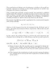
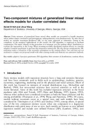
6 D. B. Hall and J. Shen Scand J StatistTable 1. Relative efficiencies for zero-inflated Poisson (ZIP) model parameters for differentvalues of the tuning quantile cZIP with γ = 1.0 ZIP with γ = 4.0c γ = 1.0 β 1 = 0 β 2 = 1 β 3 = 0.1 γ = 4.0 β 1 = 0 β 2 = 1 β 3 = 0.1c = 0.005 0.998 0.993 0.996 0.996 1.000 0.995 0.996 0.996c = 0.010 0.997 0.987 0.993 0.993 1.000 0.990 0.993 0.993c = 0.015 0.996 0.985 0.990 0.990 1.000 0.988 0.990 0.990c = 0.020 0.995 0.982 0.988 0.988 1.000 0.986 0.988 0.988c = 0.025 0.995 0.981 0.986 0.986 1.000 0.985 0.986 0.986c = 0.030 0.992 0.967 0.981 0.981 0.999 0.975 0.982 0.981c = 0.040 0.990 0.955 0.972 0.971 0.999 0.965 0.973 0.972c = 0.050 0.988 0.947 0.969 0.968 0.999 0.959 0.969 0.969c = 0.075 0.985 0.930 0.946 0.945 0.999 0.944 0.947 0.946c = 0.100 0.980 0.924 0.938 0.937 0.998 0.940 0.940 0.939particular, we consider ZIP models with non-constant mixing probability p = {1 + exp(−γg)} −1and Poisson mean μ = e Bβ . Specifically, we set g = j T 10⊗(−1.5, −1.4, −1.3, −1.2, −1.1, − 1.0,− 0.9, − 0.8, − 0.7, − 0.6) and⎛1 1 1 1 1 0 0 0 0⎞0B T = j T 10 ⊗ ⎝ 0 0 0 0 0 1 1 1 1 1 ⎠.1 2 3 4 5 6 7 8 9 10Parameters γ and β were chosen to yield some overlap between the mixture components andare listed in Table 1. Two values, 1 and 4, were chosen for γ, which give values of p in therange (0.18, 0.35) and (0.0025, 0.083), respectively.Based on these models, we report the ratios of asymptotic variances for values of c rangingfrom 0.005 to 0.10 in Table 1. Because no high leverage points exist in the data, the ratiosof asymptotic variance corresponding to the mixing probability are close to 1. Ratios for theregression parameters decrease as expected with c, but the relative efficiency for the RES estimatorsis reasonably high even for c = 0.10. In the simulation studies and example of sections4 and 5, we take c = 0.01 for the ZIP models we consider. In the simple models we considerhere, this choice leads to relative efficiencies for β of 98.7 per cent or better. Of course, therelative efficiency of the RES approach will differ across models, but the results we presenthere give some sense of the efficiency loss that one might expect in practice.3. MHD estimation in ZI regression models3.1. MHD methodThe literature on MHD estimation concentrates primarily on the i.i.d. setting. In that contextthe Hellinger distance is defined as H 2 (f n , f θ ) = ∫ {f n (y) 1/2 − f θ (y) 1/2 } 2 dy where f θ is themarginal density of a response variable Y based on a sample y 1 , ..., y n according to theparametric model under consideration and f n is a corresponding non-parametric density estimate.For discrete data, the natural choice for f n is the empirical frequency function defined byf n (y) = N y /n, y ∈ Y, (8)where N y is the number of observations having value y, and Y is the sample space for Y.In the context of Poisson mixture regression models, Lu et al. (2003) presented MHD estimatorsdefined in terms of the classical Hellinger distance between the empirical frequencyfunction f n (·) and the marginal density for Y implied by the model. Because ZIP regressionfalls in the class of models these authors considered, here we treat their approach as an© 2009 Board of the Foundation of the Scandinavian Journal of Statistics.
Scand J Statist Robust ZIP regression 7alternative robust estimation method and standard of comparison for the RES method ofsection 2. Lu et al. (2003) suggested replacing f θ (y) with a simple, but consistent estimatorf θ,n (y), defined byf θ,n (y) = 1 n∑f θ (y | x i ), y ∈ Y. (9)ni = 1This leads to an MHD estimator defined as ˆθ MHD = arg min θ∈Θ H 2 ( f θ, n , f n ).Lu et al. (2003) claim that the results of the earlier authors should extend to the finitemixture of Poisson regression context, of which the ZIP model is a special case. These authorspropose an asymptotic variance estimator of the form∂ 2 f θ, n (y)∂θ∂θ Tvar( ˆ ˆθ) = ∑ y∈Y {ˆ˙lθ (y)ˆ˙lT θ(y)f n (y) −| θ = ˆθ }, where ˆ˙lθ (y) = ∂ log f ∂θ θ,n(y)| θ = ˆθ. However, formal proofs for asymptotic propertiesof MHD estimators in the non-i.i.d. set-up have not been established.3.2. IdentifiabilityThe issue of identifiability of finite mixture models has attracted considerable attention in theliterature, but most of this discussion has centred on the likelihood function and has assumedconstant mixing probability in the model. When using MHD estimation via marginal densitiesrather than ML, however, the class of identifiable models is more restricted. In addition,ZI regression models allow a regression structure logit(p i ) = G T i γ, which invalidates many ofthe existing results and adds complexity to the identifiability question. For ZI models withnon-constant mixing probability it is not hard to find simple non-identifiable models basedon the unconditional (marginal) density. For example, let{ 0, with probability pi ,Y i ∼Poisson(μ), with probability 1 − p i ,and suppose that p i depends on X i , where X i is a binary variable,{ 0, i = 1, 2, ..,nX i =21, i = n + 1, ..., n.2It follows that p i = logit −1 (γ 1 ) ≡ P 1 if i = 1, 2, ..., n/2, otherwise p i = logit −1 (γ 2 ) ≡ P 2 . Themarginal density is f θ,n (y) = 1 (P 2 1 + P 2 )I(y = 0) + {1 − 1 (P 2 1 + P 2 )} e−μ μ y, which is clearly noty!identifiable.Necessary and sufficient identifiability conditions in the class of models are difficult toestablish. However, in our simulation studies we encountered singular Hessian matrices forthe MHD criterion for most of the models we considered that have non-constant mixingprobability.4. Simulation studiesThe aim of these simulations is to assess the performance of ML, RES and MHD estimatorsin the presence of outliers and/or poor separation of the mixture components. Becauseof non-identifiability problems with the MHD method, we restrict attention to the case ofconstant mixing probability in study 1, and consider only the RES and ML approaches fornon-constant mixing probability in simulation studies 2 and 3. In studies 1 and 2, data aregenerated from a ZIP model with outliers in the response, whereas in study 3 we generate datafrom a ZIP model and add outlying values in the explanatory variables (high leverage points).In all the three studies, two sample sizes, n = 100 and n = 200, and two different degrees ofseparation between the mixture components are examined.© 2009 Board of the Foundation of the Scandinavian Journal of Statistics.
Page 2 and 3: 2 D. B. Hall and J. Shen Scand J St
Page 10 and 11: 10 D. B. Hall and J. Shen Scand J S
Page 16: 16 D. B. Hall and J. Shen Scand J S

Robust Estimation for Zero-Inflated Poisson Regression - Franklin ...

You also want an ePaper? Increase the reach of your titles

Delete template?

Save as template?