PD / PID Control, Steady State Error, and Stability Analysis

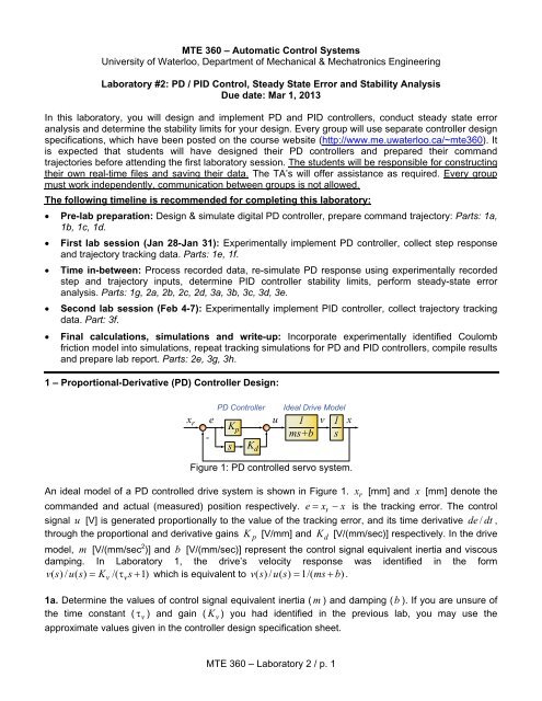
MTE 360 – Automatic Control SystemsUniversity of Waterloo, Department of Mechanical & Mechatronics EngineeringLaboratory #2: PD / PID Control, Steady State Error and Stability AnalysisDue date: Mar 1, 2013In this laboratory, you will design and implement PD and PID controllers, conduct steady state erroranalysis and determine the stability limits for your design. Every group will use separate controller designspecifications, which have been posted on the course website (http://www.me.uwaterloo.ca/~mte360). Itis expected that students will have designed their PD controllers and prepared their commandtrajectories before attending the first laboratory session. The students will be responsible for constructingtheir own real-time files and saving their data. The TA’s will offer assistance as required. Every groupmust work independently, communication between groups is not allowed.The following timeline is recommended for completing this laboratory: Pre-lab preparation: Design & simulate digital PD controller, prepare command trajectory: Parts: 1a,1b, 1c, 1d.First lab session (Jan 28-Jan 31): Experimentally implement PD controller, collect step responseand trajectory tracking data. Parts: 1e, 1f.Time in-between: Process recorded data, re-simulate PD response using experimentally recordedstep and trajectory inputs, determine PID controller stability limits, perform steady-state erroranalysis. Parts: 1g, 2a, 2b, 2c, 2d, 3a, 3b, 3c, 3d, 3e.Second lab session (Feb 4-7): Experimentally implement PID controller, collect trajectory trackingdata. Part: 3f.Final calculations, simulations and write-up: Incorporate experimentally identified Coulombfriction model into simulations, repeat tracking simulations for PD and PID controllers, compile resultsand prepare lab report. Parts: 2e, 3g, 3h.1 – Proportional-Derivative (PD) Controller Design:PD ControllerIdeal Drive Modelx r e u 1 v 1 xK p-ms+b ss K dFigure 1: PD controlled servo system.An ideal model of a PD controlled drive system is shown in Figure 1. x r [mm] and x [mm] denote thecommanded and actual (measured) position respectively. e xr x is the tracking error. The controlsignal u [V] is generated proportionally to the value of the tracking error, and its time derivative de / dt ,through the proportional and derivative gains K p [V/mm] and K d [V/(mm/sec)] respectively. In the drivemodel, m [V/(mm/sec 2 )] and b [V/(mm/sec)] represent the control signal equivalent inertia and viscousdamping. In Laboratory 1, the drive’s velocity response was identified in the formv( s) / u(s) Kv /( vs1)which is equivalent to v( s) / u(s) 1/( ms b).1a. Determine the values of control signal equivalent inertia ( m ) and damping (b ). If you are unsure ofthe time constant ( v ) and gain ( K v ) you had identified in the previous lab, you may use theapproximate values given in the controller design specification sheet.MTE 360 – Laboratory 2 / p. 1

xrsimClocktsimKp[texp xrexp]CommandInput(From Workspace)KdKpKdz-1Ts.zDiscrete DerivativeZero-OrderHoldControlSignalLimit1m.s+bdrive modelusim1sIntegrator PositionMeasurementQuantizationxsimTo Workspace1b. Determine the values of K p andFigure 2: Simulink model for PD controlled servo system.K d which result in the given specifications of natural frequencyand damping ratio for the closed loop poles. The specifications for each group have been posted onthe course website. Hint: Consider the resemblance between the closed loop transfer functiondenominator, and that of an ideal 2 nd order system.1c. Compare the closed loop step response of the PD controlled system to that of an ideal 2 nd order2 22model: x(x) / xr( s) n/( s 2ns n). Explain the similarities and/or differences between the tworesponses, elaborating with control theory and your engineering judgment. Comment on rise time andovershoot values in each case.1d. Test your controller in simulation using a Simulink model similar to the one shown in Figure 2. Notethat the pure derivative operator ( s ) in Figure 1 has been replaced with the discrete-time approximation( z 1) /( Tsz), which is also known as Euler’s approximation. T s =1 [msec] is the sampling period. TheZero-Order Hold is used to convert the discrete time control signal into continuous time. Make sure thatyou set the sampling period in the discrete derivative and ZOH blocks to T s . The control signal cannotexceed a magnitude of 10 [V]. This is reflected by incorporating a Saturation Block with limits of -10 …+10 [V]. Also, the position measurements are obtained using an incremental encoder. Considering theencoder resolution and gear specifications given in the drive’s user manual, the smallest position changethat can be detected is dx =0.023 [mm]. This is reflected in the Quantization Block. Simulate the stepresponse of the closed loop system to verify the stability of your implementation (you do not need toreport this intermediate result).1e. Implement the PD controller on the experimental setup. You may modify the file p_control.mdl, whichyou had used in Lab 1. Your implementation should look like the file shown in Figure 3. You may get helpfrom the TA in compiling your real-time Simulink file. Test the closed loop step response by applying asquare wave input with ±0.2 [mm] amplitude at 2 [Hz] frequency. Capture 2.0 [sec] of data containing thecommand ( x r ), output ( x ), and control (u ) signals. You may modify the script fileplot_p_control_result.m to extract, plot, and save the necessary signals after you transfer them from thereal-time scopes to the Matlab workspace.1f. Apply the position command shown in Figure 4, consisting of a forward and backward movement withcontrolled accelerations, as a Repeating Sequence to your closed loop system. You may modify thetrajectory generation example covered in the Matlab tutorial (posted on the course website) to generateyour reference trajectory. The displacement is 50 [mm], with 100 [mm/sec] velocity, and 500 [mm/sec 2 ]acceleration transients. There should be enough pause after each movement so that a forward andbackward cycle is completed exactly in 2.000 [sec]. During the experiment, monitor the commanded and nMTE 360 – Laboratory 2 / p. 2

Figure 3: Real-time file for PD controller implementation.Position[mm]Velocity[mm/sec]60402002001000Acceleration[mm/sec 2 ]10005000-500-10000 0.2 0.4 0.6 0.8 1.0 1.2time [sec]1.4 1.6 1.8 2.0Figure 4: Command trajectory for tracking experiments.actual position, tracking error, and control signal profiles. Capture data for 4.0 [sec] and save the profilesfor x r , x , and u .1g. Apply the experimentally recorded position commands for the step input and smooth trajectory toyour simulation (Figure 2). Present the results separately for each case. Overlay the simulated andexperimental results on top of each other. You graphs should be in the following format:1) Position trajectory: x r and x versus t (on the top);2) Tracking error: e versus t (in the middle);3) Control signal: u versus t (on the bottom).All time axes should be common, hence the signals need to be synchronized. Comment on thesimilarities and/or discrepancies between the simulation and experimental results. Support yourcomments with control theory and your engineering judgment.MTE 360 – Laboratory 2 / p. 3

2 – Steady State Error Analysis*** This section can be completed after finishing the first lab session. ***Drive with Disturbance InputPD Controller dx r e u - 1 v 1 xK p-ms+b ss K dFigure 5: PD controlled system with disturbance input.A more realistic drive model would also include the effect of friction as a second input, as shown inFigure 5. In the figure, d [V] represents the control signal equivalent disturbance, which mainlyoriginates from the Coulomb friction in the drive mechanism, when other disturbance forces are notapplied. Considering that the magnitude of Coulomb friction should ideally be constant ( d c [V]), thedisturbance model can be expressed as:1 if v 0d dc sgn( v), where sgn(v) 0 if v 0(1)1if v 02a. Express the drive position x as a function of both the trajectory command x r , as well as the controlsignal equivalent disturbance input d in the form: x( s) Gxrx ( s) xr( s) Gdx( s) d(s). In servocontrol literature, Gxr x (s ) is frequently referred to as the tracking transfer function, and G d x (s)isreferred to as the disturbance transfer function.2b. The performance of a controller is usually evaluated based on how small the following error can bemade in the presence of various command and disturbance inputs. Express the tracking error e as afunction of the command x r and disturbance d in the form: e( s) Gxr e(s) xr( s) Gde(s) d(s).2c. Including the effect of Coulomb friction, determine the theoretical expression for steady statefollowing error during constant velocity motion. Hint 1: You will need to use the Final Value Theorem.Hint 2: Use the principle of superposition to break the steady state error into two components:e ss ess_ traj ess_ fric , where e ss _ traj represents the steady state error due to a constant velocitycommand and e ss _ fric represents the steady state error due to opposing Coulomb friction. Elaborate onhow these error components are affected by the commanded velocity v ref , friction magnitude d c , driveparameters m and b , controller gainsK p andK d , and the closed loop natural frequency n [rad/sec].2d. Carefully observe the experimental tracking result recorded in Part 1f, particularly the value offollowing error during constant velocity motion. Use the formulation developed in Part 2c to determine theaverage value of Coulomb friction (in terms of equivalent control signal) d c [V] in your experimentalsetup. Explain your methodology in the calculations. Also indicate the theoretical value of steady statetracking error in the absence of friction.MTE 360 – Laboratory 2 / p. 4

xrsimtsimClockCoulomb frictionKpf(u)[texp xrexp]CommandInput(From Workspace)KdKpKdz-1Ts.zDiscrete DerivativeZero-OrderHoldControlSignalLimit1m.s+bdrive modelusim1sIntegrator PositionMeasurementQuantizationxsimTo WorkspaceFigure 6: Simulink model of PD controlled system with Coulomb friction.2e. Incorporate the effect of Coulomb friction into your simulation, as shown in Figure 6. You may use aUser Defined Function in Simulink for implementing the friction model in Equation 1. Re-run yoursimulation using the experimentally recorded smooth command trajectory in Part 1f, and overlay thesimulated and experimental tracking results once more (Part 1g). Comment on the similarity and/ordiscrepancy between the simulation and experimental results.3 – Proportional – Integral – Derivative (PID) Control and Stability Analysis:PID ControllerDrive with Disturbance InputK pdx r e 1 u - 1 v 1K xs i-ms+b ssK dFigure 7: PID controlled drive system.Integral action is frequently used in control systems to eliminate steady state tracking error. By adding anintegrator with a gain K i [V/(mmsec)] to the PD controller, a Proportional – Integral – Derivative (PID)controller is obtained, as shown in Figure 7. Assuming that the integral gain is nonzero:3a. Express the drive position x as a function of trajectory command x r and disturbance input d (i.e.re-derive the tracking and disturbance transfer functions Gxr x (s ) and G d x (s)).3b. Derive the expressions for theoretical steady state error values e ss _ traj and e ss _ fric .3c. Using Routh’s Stability Criterion, derive the mathematical expressions for the PID gains K p ,and K d which will guarantee the stability of the closed loop system in Figure 7.3d. Using the PD gains you computed in Part 1b, determine the upper limit for the integral gain K i max ,required to hold stability. Verify in simulation that an integral gain above this limit (for exampleKi 1.2Kimax ) will result in an unstable response. In constructing your Simulink model, you mayapproximate the integrator in discrete-time using the Euler technique: 1/s Ts z /( z 1). Report yoursimulation result for the smooth trajectory input in accordance with the format in Part 1g. Remember toinclude the Coulomb friction (after you have identified its value) into your simulation.K i ,MTE 360 – Laboratory 2 / p. 5

Figure 8: Real-time file for PID controller implementation.3e. Simulate the tracking response of your PID controller for different values of the integral gain. Stateyour observations on how the following error is affected as you modify K i . Report two or threecharacteristically different cases. Use the format given in Part 1g.3f. Implement and test your PID controller on the experimental setup, as shown in Figure 8. To have areasonable amount of integral action, while also guaranteeing stability, set Ki K i max / 3 as a rule ofthumb. Use the smooth trajectory in Figure 4 as the input. Capture the profiles for x r , x , and u for aduration of 4.0 [sec], as you did in to Part 1f. Using the commanded trajectory recorded during theexperiment, and the same value for integral gain ( K i max / 3 ), conduct the tracking simulation. Show thesimulation and experimental results on top of each other, as described in Part 1g. Elaborate on thesimilarities and/or differences between the two.3g. Overlay the experimental results obtained in Parts 1f and 3f on top of each other. Comment on thecontribution of integral action to the servo performance. Does integral control provide better tracking anddisturbance rejection? What are the limitations? You may refer to your calculations and mathematicalderivations from Parts 2c, 3b, 3c to back up your comments.3h. Plot pole-zero maps of the PD and PID controlled closed loop tracking transfer functions on the samegraph. Use different line styles (or preferably colors) to distinguish the two cases. Comment on the poleand zero locations, also referring to natural frequency and damping ratio values. You may use the Matlabcommands pzmap() and damp() to assist in your calculations. Indicate how the closed loop polelocations are affected with the introduction of integral action.Report format and submission: Every group will submit one report, both in electronic and hard-copyformats. The electronic report will be e-mailed to the TA (aokyay@uwaterloo.ca) no later than 5 pm onthe due date. Hard copies of the reports must also be submitted by the same deadline. There should beno discrepancy between the electronic and printed reports. Equations, figures, and tables should bepresented neatly and clearly. They should either be prepared using appropriate software, or neatlywritten (or drawn) by hand and scanned into the report. To keep the report length short, your commentsshould be in bullet form, when possible. The reports should only present the requested data andcomments. They should be brief; no longer than 8 pages (excluding appendices), written in Arial 10 pt.fonts. Matlab code and Simulink block diagrams should be presented in the appendix. TOC, LOT, LOF,Introduction, and Conclusions sections are not necessary. However, it is important that you follow thesame heading numbers with the lab handout when presenting your answers.MTE 360 – Laboratory 2 / p. 6

Lab reports will be marked based on correctness of the experimental procedure and theoretical analyses,calculations, presentation of data, and correct engineering comments. The format and quality of thereport will also be taken into consideration. Late submissions will receive 10% penalty per day.MTE 360 – Laboratory 2 / p. 7