TASI Lectures on Flavor Physics (June 2008) - University of ...

<strong>TASI</strong> <strong>Lectures</strong> on Flavor Physics(June 2008)K.S. BabuLecture I

§1. OverviewThis set of lectures will focus on the flavor sector of the Standard Model (SM). As you know,most of the free parameters of the SM reside in this sector. In case you have not thought of itlately, let me remind you of the counting of parameters. Not including neutrino masses, thereare 19 parameters in the SM. Five of these are flavor universal – the three gauge couplings,one Higgs quartic coupling λ, and one Higgs mass-squared µ 2 , while the remaining fourteen areflavor parameters. Six quark masses, three charged lepton masses, four quark mixing parameters(includes one CP violating phase) make up thirteen, while the strong CP violating parameterθ, which is intimately related to the quark masses, is the fourteenth flavor parameter. If weinclude small neutrino masses and neutrino mixings, as suggested by experiments, an additionalnine parameters will have to be introduced (three neutrino masses, three neutrino mixing anglesand three CP violating phases, in the case of Majorana neutrinos).While there is abundant information on the numerical values these parameters take, afundamental understanding of the parameters is currently lacking. Why are there so manyfree parameters? Why do these parameters exhibit a strong hierarchical structure spanningsome six orders of magnitude? Are the mixing parameters related to the mass ratios? Whyis θ < 10 −9 ? What is the origin of CP violation? The lack of understanding of such issues isoften referred to as the “flavor puzzle”. Various solutions to this puzzle have been proposed,inevitably leading to beyond the Standard Model, for within the SM these parameters can onlybe accommodated, and not explained. Forthcoming experiments, especially at the LHC, havethe potential to confirm or refute many, but not all, of these proposed non–standard scenarios.The Higgs boson is waiting to be discovered at the LHC. Its production and decay rates canbe significantly modified relative to the SM expectations in some of the flavor–extensions ofthe SM. I will describe explicit models in this category. Very little is known about the topquark properties currently. LHC will serve as a top factory where modifications in the topsector arising from flavor–extensions can be studied. We have learned a lot about the B mesonsystem from the B factories lately, but there are still many open issues which will be probed atthe LHC. These include precise determinations of the CP violating parameters, rare processesallowed in the SM but not yet observed, and new physics processes in B decays that requiremodification of the SM structure.In Lecture I, we will take a tour of the flavor parameters of the SM and review how these aremeasured and interpreted. Various ideas attempting to understand aspects of the flavor puzzlewill then be introduced. Experimental consequences of these ideas will be outlined. In LectureII we will pursue such ideas further and seek their tests. Lecture III will be devoted to thestatus and expectations of the Standard Model quark mixings and CP violation. Lecture IV will1

deal with beyond the SM scenarios for the flavor sector and their experimental manifestationsat the LHC.§2. Flavor structure of the Standard ModelFermion masses arise in the SM via Yukawa interactions given byL Yukawa = Q T Y u u c H − Q T Y d d c ˜H − L T Y l e c ˜H + h.c. (1)Here I have used the standard notation for quark (Q,u c ,d c ) and lepton (L,e c ) fields. (Q, L)are SU(2) L doublets as is the Higgs field H, and its cousin ˜H = iτ 2 H ∗ , while the (u c , d c , e c )fields are SU(2) L singlets. All fermion fields are left–handed, a charge conjugation matrixC is understood to be sandwiched between all of the fermion bilinears. Contraction of thecolor indices is not displayed, but should be obvious. Y u,d,l are the Yukawa couplings matricesspanning generation space which are complex and non–Hermitian. SU(2) L contraction betweenthe fermion doublet and Higgs doublet involves the matrix iτ 2 . Explicitly, we have for familylabeled by index iQ i =so that Eq. (1) expands to( ) ( ) ( ui νi H+ ) ( H; L i = ; H = ; ˜H0 )=d i e i H 0 −H −L Yukawa = (Y u ) ij [u i u c jH 0 −d i u c jH + ]+(Y d ) ij [u i d c jH − +d i d c jH 0 ]+(Y l ) ij [ν i e c jH − +e i e c jH 0 ]+h.c. (3)The neutral component of H acquires a vacuum expectation value (VEV) 〈H 0 〉 = v, spontaneouslybreaking the electroweak symmetry (v ≃ 174 GeV). The Higgs field can then beparametrized as H 0 = ( h √2+ v) where h is a real physical field (the Higgs boson). In theunitary gauge H ± , which are eaten up by the W ± gauge bosons and the phase of H 0 , which iseaten up by the Z 0 gauge boson, do not appear.The VEV of H 0 generates the following fermion mass matrices:M u = Y u v, M d = Y d v, M l = Y l v . (4)The Yukawa coupling matrices contained in (Y u ) ij / √ 2(uu c h), etc in each of the up, down andcharged lepton sector becomes proportional to the corresponding mass matrix. Once the massmatrices are brought to diagonal forms, the Yukawa coupling matrices will also be brought todiagonal forms. There is thus no tree–level flavor changing current mediated by the neutralHiggs boson in the Standard Model. As we will see, this feature is generally lost as we extendthe SM to address the flavor issue.(2)2

We make unitary rotations on the quark fields in family space. Unitarity of these rotationwill ensure that the quark kinetic terms remain canonical. Specifically, we define masseigenstates (u 0 ,u c0 ,d 0 ,d c0 ) viaand we choose the unitary matrices such thatVu T(Y u v)V u c = ⎜⎝u = V u u 0 , u c = V u c u c0 ,d = V d d 0 , d c V d c d c0 (5)⎛⎞m um cm t⎟⎠ , V d T(Y d v)V d c = ⎜⎝⎛⎞m dm sm b⎟⎠ . (6)We have assumed here that the number of families is three, but the procedure applies to anynumber of families. Bi-unitary transformations such as the ones in Eq. (6) can diagonalizenon–Hermitian matrices. The same transformations should be applied to all interactions of thequarks. As already noted, this transformation will bring the Yukawa interactions of quarks withthe Higgs boson into diagonal form. The couplings of the Z 0 boson and the photon to quarkswill have the original diagonal form even after this rotation. For example, (uγ µ Iu)Z µ whereI is the identity matrix acting on family space will transform to (u 0 γ µ (V †uIV u )u 0 )Z µ , which isidentical to (u 0 γ µ Iu 0 )Z µ . Similarly, (u c γ µ Iu c )Z µ will transform to (u c0 γ µ Iu c0 )Z µ . We see thatthere is no tree level flavor changing neutral current (FCNC) mediated by the Z 0 boson andthe photon in the SM.Most significantly, the transformations of Eq. (6) will bring the charged current quarkinteraction, which originally is of the form g/ √ 2(uγ µ d)W +µ + h.c., into the formwhereL cc = g √2[u 0 γ µ V d 0 ] W µ+ + h.c. (7)V = V †uV d (8)is the quark mixing matrix, or the Cabibbo–Kobayashi–Maskawa (CKM) matrix. In the SM,all the flavor violation is contained in V . Being product of unitary matrices, V is itself unitary.This feature has thus far withstood experimental scrutiny, with further scrutiny expected fromLHC experiments.Note that the right–handed rotation matrices V u c and V d c have completely disappeared, aresult of the purely left–handed nature of charged weak current.We can repeat this process in the leptonic sector. We define, in analogy with Eq. (5),ν = V ν ν 0 , e = V e e 0 , e c = V e c e c0 . (9)3

We choose Y e and Y e c such thatYe T(Y l v)Y e c = ⎜⎝⎛⎞m em µm τ⎟⎠ . (10)Note that there is no right–handed neutrino in the SM. If the Yukawa Lagrangian is asgiven in Eq. (1), there is no neutrino mass. In that case one can choose V ν = V e , so that thecharged current weak interactions will remain flavor diagonal. However, it is now establishedthat neutrinos have small masses. Additional terms must be added to Eq. (1) in order toaccommodate them. The simplest possibility is to add a non–renormalizable termL ν mass = (LT Y ν L)HHM ∗(11)where the SU(2) L contraction between the H fields is in the triplet channel and Y ν is a complexsymmetric matrix in generation space. Here M ∗ is a mass scale much above the weak interactionscale. Eq. (11) can arise by integrating out some heavy fields with mass of order M ∗ . Themost celebrated realization of this is the seesaw mechanism, where M ∗ corresponds to the massof the right–handed neutrino. The neutrino masses are suppressed, compared to the chargedfermion masses, because of the inverse dependence on the heavy scale M ∗ . Right–handedneutrinos, if they exist, are complete singlets of the SM gauge symmetry, and can possess bareSM invariant mass terms, unlike any other fermion of the SM. This is an elegant explanation ofwhy the neutrinos are much lighter than other fermions, relying only on symmetry principlesand dimensional analysis. Eq. (11) leads to a light neutrino mass matrix given byM ν = Y νv 2M ∗. (12)Now we choose V ν so thatVν T v 2Y ν V ν = ⎜M⎝∗⎛⎞m 1m 2m 3⎟⎠ , (13)with m 1,2,3 being the tiny masses of the three light neutrinos. The leptonic charge currentinteraction now becomesL l cc = g √2[e 0 γ µ Uν 0 ] W −µ + h.c. (14)whereU = V †e V ν (15)4

is the leptonic mixing matrix, or the Pontecorvo–Maki–Nakagawa–Sakata (PMNS) matrix.As V , U is also unitary. Neutrino oscillations observed in experiments are attributed to theoff–diagonal entries of the matrix U. We assumed here that the neutrino mass generationmechanism violated total lepton number by two units. While this is very attractive, it shouldbe mentioned that neutrinos could acquire masses very much like the quarks do. That wouldrequire the right–handed ν c states to be part of the low energy theory. M ν will then be similar toM l of Eq. (10). Neutrino oscillation phenomenology will be identical to the case of L–violatingneutrino masses.The fermionic states (e 0 i) are simply the physical electron, the muon, and the tau leptonstates. Similarly, the quark fields with a superscript 0 are the mass eigenstates. It is conventionalto drop these superscripts, which we shall do from now on.§3. Lepton massesConceptually charged lepton masses are the easiest to explain. Leptons are propagatingstates, and their masses are simply the poles in the propagators. Experimental information oncharged lepton masses is rather accurate:m em µ= 0.510998902 ± 0.000000021 MeV= 105.658357 ± 0.000005 MeVm τ = 1777.03 +0.30−0.26 MeV . (16)The direct kinematic limits on the three neutrino masses are:m νe ≤ 3 eV, m νµ ≤ 0.19 MeV, m ντ ≤ 18.2 MeV . (17)Neutrino oscillation experiments have provided much more accurate determinations of thesquared mass differences ∆m 2 ij = m 2 i − m 2 j. Solar and atmospheric neutrino oscillation experimentssuggest the following allowed values (with 2σ error quoted):∆m 2 21 = (7.3 − 8.1) × 10 −5 eV 2∆m 2 31 = ±(2.1 − 2.7) × 10 −3 eV 2 . (18)While this still leaves some room for the absolute masses, when combined with the direct limiton m νe ≤ 3 eV, the options are limited. Current data allows for two possible ordering of themass hierarchies: (i) normal hierarchy where m 1 ≤ m 2 ≪ m 3 , and inverted hierarchy wherem 1 ≃ m 2 ≫ m 3 .§4. Leptonic mixing matrixThe PMNS matrix, being unitary, has N 2 independent components for N families of leptons.Out of these, N(N − 1)/2 are Euler angles, while the remaining N(N + 1)/2 are phases. Many5

of these phases can be absorbed into the fermionic fields and removed. If one writes U = QÛP,where P and Q are diagonal phase matrices, then by redefining the phases of e fields Q,which has N phases, can be removed. P has only N − 1 non–removable phases. For N = 3,P = diag.(e iα , e iβ , 1). α,β are called the Majorana phases. (If the neutrino masses are ofthe Dirac type, these phases can also be removed by redefining the ν c fields.)Û will then haveN(N + 1)/2 − (2N − 1) = 1 (N − 1)(N − 2) phases. For N = 3, there is a single “Dirac” phase2in U.In general, the PMNS matrix can be written as⎛⎞U e1 U e2 U e3U = ⎜⎝ U µ1 U µ2 U µ3⎟⎠ . (19)U τ1 U τ2 U τ3To enforce the unitarity relations it is convenient to adopt specific parametrizations. TheEuler angles, as you know, can be parametrized in many different ways. Furthermore, theDirac phase can be chosen to appear in different ways (by field redefinitions). The “standardparametrization” that is now widely used has U PMNS = U.P where⎛c 12 c 13 s 12 c 13 s 13 e −iδ ⎞U = ⎜⎝ −s 12 c 23 − c 12 s 23 s 13 e iδ c 12 c 23 − s 12 s 23 s 13 e iδ s 23 c 13⎟⎠ . (20)s 12 s 23 − c 12 c 23 s 13 e iδ −c 12 s 23 − s 12 c 23 s 13 e iδ c 23 c 13Here s ij = sin θ ij , c ij = cos θ ij .Our current understanding of these mixing angles arising from neutrino oscillations can besummarized as follows (2 σ error bars quoted):sin 2 θ 12 = 0.28 − 0.37sin 2 θ 23 = 0.38 − 0.63sin 2 θ 13 ≤ 0.033 . (21)Here θ 12 limit arises from solar neutrino data, θ 23 from atmospheric neutrinos, and θ 13 fromreactor neutrino data.It is intriguing that the current understanding of leptonic mixing can be parametrized bythe unitary matrix⎛U MNS = ⎜⎝√ 23√130− 1 √61 √3 − 1 √2− 1 √61 √3 1⎞⎟⎠ P . (22)√2This mixing is known as tri-bimaximal mixing. As we will see, such a geometric structure isfar from being similar to the quark mixing matrix. Note that currently θ 13 is allowed to be6

zero, in which case the Dirac phase δ becomes irrelevant. We also have no information on theMajorana phases, which can only be tested in neutrinoless double beta decay experiments.§5. Quark massesUnlike the leptons, quarks are not propagating particles. So their masses have to be inferredindirectly from properties of hadrons. There are various techniques to do this. Let me illustratethis for the light quark masses by the method of chiral perturbation theory.Consider the QCD Lagrangian at low energy scales. Electroweak symmetry has alreadybeen broken, and heavy quarks (t,b,c) have decoupled. The Lagrangian takes the formL =N F ∑k=1q k (i̸D − m k )q k − 1 4 G µνG µnu (23)where G µν is the gluon field strength and ̸D is the covariant derivative. m k is the mass of thekth quark and q k the quark field. This Lagrangian has a chiral symmetry in the limit wherethe quark masses vanish. The symmetry is SU(3) L × SU(3) R × U(1) V , with the axial U(1) Aexplicitly broken by anomalies. The U(1) V is baryon number, which remains unbroken evenafter QCD dynamics. QCD dynamics breaks the SU(3) L ×SU(3) R symmetry down to SU(3) V .In the limit of vanishing quark masses, there must be 8 Goldstone bosons corresponding to thissymmetry breaking. These Goldstone bosons are identified as the pseudoscalar mesons, whichare however, not exactly massless. The quark masses break the chiral symmetry explicitly andthus generate masses for the mesons.Chiral perturbation theory is a systematic expansion in p/Λ χ , where p is the particle momentumand Λ χ ∼ 1 GeV is the chiral symmetry breaking scale. Since the masses of the lightquarks (u, d, s) are smaller than Λ χ , we can treat them to be small and apply chiral expansion.The explicit breaking of chiral symmetry occurs via the mass term⎛⎞m um dm sM =⎜⎝⎟⎠ . (24)M can be thought of as a field which broke the chiral symmetry spontaneously. M can be splitas M = M 1 + M 8 , where M 1 is a singlet under SU(3) V , while M 8 transforms as an octet:⎛ ⎞1M 1 = (m u + m d + m s )⎜3⎝ 1 ⎟⎠ ,1⎛ ⎞⎛ ⎞M 8 = (m u − m d )2⎜⎝1−1⎟⎠ + (m u − m d − 2m s )⎜6⎝0711−2⎟⎠ (25)

The octet of mesons can be written down as a (normalized) matrixΦ =⎛⎜⎝π 0 √2+ η0 √6π + K +π −− π0 √2+ η0 √6K 0K − K 0 − √ 2The lowest order invariants involving Φ bilinear and M are3 η0 ⎞⎟⎠ . (26)A Tr(Φ 2 )M 1 + B Tr(Φ 2 M 8 ) . (27)A and B are arbitrary coefficients here. Eq. (27) can be readily expanded, which will giverelations for the masses of mesons. Now, in the limit of m u = 0,m d = 0,m s ≠ 0, the SU(2) L ×SU(2) R chiral symmetry remains unbroken, and so the pion fields should be massless. Workingout the mass terms, and demanding that the pion mass vanishes in this limit, gives a relationA = 2B. Using this relation we can write down the pseudoscalar meson masses. In doing so, letus also recall that electromagnetic interactions will split the masses of the neutral and chargedmembers. To lowest order, this splitting will be universal. Then we havem 2 π 0 = B(m u + m d )m 2 π ±= B(m u + m d ) + ∆ emm 2 K 0 = m2 K 0 = B(m d + m s )m 2 K ±= B(m u + m s ) + ∆ emm 2 η = 1 3 B(m u + m d + 4m s ) (28)Here small π 0 − η 0 mixing has been neglected, which vanishes in the limit m u − m d vanishes.Eliminating B and ∆ em from Eq. (28) we obtain two relations for quark mass ratios:m um d= 2m2 π− m 2 0 π+ m 2 + K− m 2 + K 0= 0.56m 2 K− m 2 0 K+ m 2 + π +m sm d= m2 K+ m 2 0 K− m 2 + π += 20.1m 2 K− m 2 0 K+ m 2 + π + (29)This is the lowest order chiral perturbation theory result for these mass ratios. Note that theabsolute masses cannot be determined in this way. QCD sum rules and lattice calculations areneeded for this.For heavy quarks (c and b), one can invoke heavy quark effective theory (HQET). Whenthe mass of the quark is heavier than the typical momentum of the partons Λ ∼ m p /3 = 330MeV, one can make another type of expansion. In analogy with atomic physics, where differentisotopes exhibit similar chemical behavior, the behavior of charm hadrons and bottom hadrons8

will be similar. In fact, there will be an SU(2) symmetry relating the two, to lowest order inHQET expansion. One consequence is that the mass splitting between the vector and scalarmesons in the b and c sector should be the same. This leads to a relations M B ∗ −M B = Λ 2 /m band M D ∗ − M D = Λ 2 /m c , leading to the predictionin good agreement with experiments.M B ∗ − M BM D ∗ − M D= m cm b(30)There is general agreement with these types of evaluations and lattice QCD calculations,which are perhaps more reliable. Listed below are the masses of quarks obtained from latticeQCD:§6. Quark mixing12 (m u + m d )(2 GeV) = 3.8 ± 0.8 MeVm s (2 GeV = 95 ± 20 MeVm c (m c ) = 1.30 ± 0.20 GeVm b (m b ) = 4.20 ± 0.20 GeV (31)The unitary matrix V of Eq. (8) appears in a variety of processes. A lot of information hasbeen gained on the matrix elements. The general matrix can be written as⎛⎞V ud V us V ubV = ⎜⎝ V cd V cs V cb⎟⎠ . (32)V td V ts V tbThe standard parametrization of V is as in Eq. (20), but now understood to be for the quarksector. V has a single un-removable phase for three families of quarks and leptons. This allowsfor the violation of CP symmetry in the quark sector. Unlike in the leptonic sector, the quarkmixing angles turn out to be small. This enables one to make a perturbative expansion of themixing matrix a la Wolfenstein. The small parameter is taken to be λ = V us in terms of whichone has⎛1 − 1 2 λ2 − 1 8 λ4 λ Aλ 3 ⎞(ρ − iη)V = ⎜⎝ −λ 1 − 1 2 λ2 − 1 8 λ4 (1 + 4A 2 ) Aλ 2⎟⎠ + O(λ5 ). (33)Aλ 3 (1 − ρ − iη) −Aλ 2 + 1 2 Aλ4 (1 − 2(ρ + iη)) 1 − 1 2 A2 λ 4Here we have the exact correspondence with Eq. (20) as given bys 12 ≡ λ, s 23 ≡ Aλ 2 , s 13 e −iδ ≡ Aλ 3 (ρ − iη) . (34)9

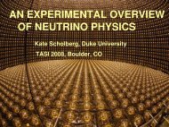
Matrix elements of V are determined usually via semileptonic decays of quarks. In Fig. 1we have displayed the dominant processes enabling determination of these elements. Fig. 1 (a)is the diagram for nuclear beta decay, from which |V ud | has been extracted rather accurately:|V ud | = 0.97377 ± 0.00027 . (35)Fig. 1 (b) shows semileptonic K decay, which yields the Cabibbo angle V us to be|V us | = 0.2257 ± 0.0021 . (36)V cd is determined from D → Klν and D → πlν with assistance from lattice QCD for thecomputation of the relevant form factors. Both V cd and V cs have rather large errors:|V cd | = 0.230 ± 0.011|V cs | = 0.957 ± 0.010 . (37)V cb is determined from both inclusive and exclusive decays of B hadrons into charm, yielding avalueV ub s determined from charmless B decays and gives|V cb | = (41.6 ± 0.6) × 10 −3 . (38)|V ub | = (4.31 ± 0.30) × 10 −3 . (39)Elements V td and V ts cannot be currently determined, for a lack of top quark events, butcan be inferred from B meson mixings where these elements appear through the box diagram.The result is|V td | = (7.4 ± 0.8) × 10 −3|V td |= 0.208 ± 0.008 . (40)|V ts |Fig. 1 (f) depicts the decay of top quark into W + b. It can also decay into W + q whereq is d,s,b. By taking the ratio of branching ratios R = B(t → Wb)/ ∑ q B(t → Wq), CDF andD0 have arrived at a limit on |V td | > 0.79.The global fits to the Wolfenstein parameters (which includes information from CP violatingobservables) can be summarized as follows:λ = 0.2272 ± 0.0010, A = 0.818 +0.007−0.017, ρ = 0.221 +0.064−0.028, η = 0.340 +0.017−0.045 (41)10

nde+KseWWuu dV usV ud νuueνeπ opD + B dllbcWWddVV cbcdνν cldlπ o DBtlbWWdV tbV ub(a)(c)(b)(d)+πu(e)νlb(f)Figure 1: Processes determining V ij .§7. Relating quark mixings and masses with flavor symmetryIn the quark sector we have seen that the mass ratios such as m d /m s , m u /m c , etc arestrongly hierarchical, while the mixing angles, such as V us are also hierarchical, although thehierarchy here is not as strong. Can the quark mixing angle be computed in terms of the quarkmass ratios? Clearly such attempts have to go beyond the SM. Here I give a simple two–familyexample which assumes a flavor U(1) symmetry that distinguishes the two families.Consider the mass matrices for (u, c) and (d, s) quarks given byM u =( ) ( )0 Au 0 Ad, MA ∗ d = , . (42)u B u A ∗ d B d11

The crucial features of these matrices are (i) the zeros in the (1,1) entries, and (ii) their hermiticity.Neither of these features can be realized within the SM. The zero entries can be enforced bya flavor U(1) symmetry, the hermitian nature can be obtained if the gauge sector is left–rightsymmetric. Before constructing such a model, let us examine the consequences of Eq. (42).Matrices in Eq. (42) have factorizable phases. That is, M u = P u ˆMu Pu, ∗ where ˆM u has the sameform as M u but with all entries real, and where P u = diag(e ıαu , 1) is a diagonal phase matrix.A similar factorization applies to M d with a phase matrix P d = diag(e ıα d , 1). We can absorbthese phase matrices into the quark fields, but since α u ≠ α d , the matrix PuP ∗ d = diag.(e ıφ , 1)will appear in the charged current matrix (φ = α d −α u ). The matrices ˆM u and ˆM d , which haveall real entries, can be diagonalized readily yielding for the mixing angles θ u and θ dtan 2 θ utan 2 θ d= m um c= m dm s(43)This yields a prediction for the Cabibbo angle| sin θ C | ≃∣√mdm s− e iφ √mum c∣ ∣∣∣∣. (44)This formula works rather well, especially since even without the second term, the Cabibboangle is correctly reproduced. The phase φ is a parameter, however, its effect is rather restricted.√√For example, since m d /m s ≃ 0.22 and m u /m c ≃ 0.07, | sin θ C | must lie between 0.15 and0.29, independent of the value of φ.Now to a possible derivation of Eq. (42). Since SM interactions do not conserve Parity,it is useful to extend the gauge sector to the left-right symmetric group SU(3) C × SU(2) L ×SU(2) R ×U(1) B−L , wherein Parity invariance can be imposed. The (2,3) and (3,2) elements ofM u,d being complex conjugates of each other will then result. The left–handed and the right–handed quarks transform as Q iL (3, 2, 1, 1/3)+Q iR (3, 1, 2, 1/3). Under discrete parity operationQ iL ↔ Q iR . This symmetry can be consistently imposed, as W L ↔ W R in the gauge sectorunder Parity. The Higgs field that couples to quarks should be Φ(1, 2, 2, 0), and under ParityΦ → Φ † . In matrix form Q iL ,Q iR , Φ read asQ iL =( uid i)Lso that the Yukawa Lagrangian, Q iR =( uid i)R, Φ =( φ01 φ + 2φ − 1 φ 0 2)(45)L Yukawa = Q L ΦY Q R + h.c. (46)12

is invariant. Imposing Parity, we see that the Yukawa matrix Y must be hermitian, Y = Y † ,which is the desired result.To enforce zeros in the (1,1) entries of M u,d , we can employ the following U(1) flavorsymmetry: Q 1L : 2, Q 1R : −2. Q 2L : 1, Q 2R : −1. Φ 1 : 2, Φ 2 : 3. Note that two Higgs bidoubletfields are needed. Φ 1 generates the (2,2) entries, while Φ 2 generates the (1,2) and (2,1) entries.There is no (1,1) entry generated, since there is no Higgs field with U(1) charge of +4.The U(1) flavor symmetry and the left–right symmetry, which were crucial for the derivation,could show up as new particles at the LHC. In general, one would also expect multiple Higgsbosons.Eq. (42) can be generalized for the case of three families, a la Fritzsch. The up and downquark mass matrices have hermitian nearest neighbor interaction form:⎛ ⎞0 A 0M u,d = ⎜⎝ A ∗ 0 B ⎟⎠0 B ∗ Cu,d. (47)These matrices preserve the prediction for Cabibbo angle of Eq. (44). In addition, this modelpredicts the following relations:|V cb | ≃∣√msm b− e iχ √mcm t∣ ∣∣∣∣,|V ub ||V cb | ≃ √mum c,|V td ||V ts | ≃ √mdm s. (48)Here χ is an undetermined phase. The relation for |V cb | would predict a top quark mass oforder (40 − 60) GeV, which is now excluded.There have been attempts to fix the problem of Fritzsch mass matrices by modifying itsform slightly. If small (2,2) elements are allowed in M u,d , the troublesome relation for V cb willbe removed, while all other predictions will stay. A different alternative is to make the (2,3)and (3,2) entries different, while maintaining the relations between (1,2) and (2,1) entries. Thiscan be achieved by non–Abelian discrete symmetries.§8. Frogatt–Nielsen mechanism for mass and mixing hierarchyThe hierarchy in the masses and mixings of quarks and leptons can be understood byassuming a flavor U(1) symmetry under which the fermions are distinguished. In this approachdeveloped by Frogatt and Nielsen, there is a “flavon” field S, which is a scalar, usually a SMsinglet field, which acquires a VEV and breaks the U(1) symmetry. This symmetry breakingis communicated to the fermions at differen order in a small parameter ɛ = 〈S〉 /M ∗ . Here M ∗is the scale of flavor dynamics, and usually is associated with some heavy fermions which areintegrated out. The nice feature of this approach is that the mass and mixing hierarchies will13

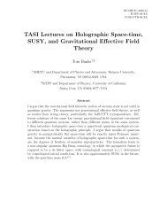
e explained as powers of the expansion parameter ɛ. The effective theory below M ∗ is rathersimple, while the full theory will have many heavy fermions, called Frogatt–Nielsen fields.Let me illustrate this idea with a two family example which is realistic when applied to thesecond and third families of quarks. Consider M u and M d for the (c, t) and (s, b) sectors givenby( ɛ4ɛ 2 ) ( ɛ3ɛ 3 )M u = v, Mɛ 2 d = v . (49)1ɛ ɛHere ɛ ∼ 0.2 is a flavor symmetry breaking parameter. Every term has an order one coefficientwhich is not displayed. We obtain from Eq. (49) the following relations for quark masses andV cb :m cm t∼ ɛ 4 ,m sm b∼ ɛ 2 , |V cb | ∼ ɛ 2 . (50)All of these relations work well, for ɛ ∼ 0.2. Although precise predictions have not been made,qualitative understanding of the hierarchies has been made.How do we arrive at Eq. (49)? We do it in two stages. First, let us look at the effectiveYukawa couplings, which can be obtained from the LagrangianL FN = [ Q 3 u c 3H u + Q 2 u c 3H u S 2 + Q 3 u c 2H u S 2 + Q 2 u c 2H u S 4]+ [ Q 3 d c 3H d S + Q 3 d c 2H d S + Q 2 d c 2H d S 3 + Q 2 d c 3H d S 3] + h.c. (51)Here I assumed supersymmetry, so that there are two Higgs doublets H u,d . It is not necessaryto assume SUSY, in that case identify H u as H of SM, and replace H d by ˜H. In Eq. (51) allcouplings are taken to be order one. The symmetry of Eq. (51) is a U(1) with the followingcharge assignment.{Q 3 ,u c 3} : 0; {Q 2 ,u c 2} : 2; {d c 2,d c 3} : 1; {H u ,H d } : 0; S : −1 . (52)Now we wish to obtain Eq. (52) by integrating out certain Frogatt–Nielsen fields. This isdepicted in Fig. 2 via a set of “spaghetti” diagrams. As you can see, there are a variety offields denoted by G i ,G i (i = 1 − 4) for the up–quark mass generation. G i have the same gaugequantum numbers as teh u c quark of SM, while G i have the conjugate quantum numbers. F ihave the quantum numbers of d c quark, while F i the conjugate quantum numbers.You can readily read off the flavor U(1) charges of the various F i and G i fields from thespaghetti diagrams.Actually the flavor U(1) that we used is anomalous. String theory generically gives ananomalous U(1) A where anomaly cancellation occurs by the Green–Schwartz mechanism. Inthis case, we can get rid of the complicated Frogatt–Nielsen fields, and simply write down14

Field U(1) A Charge Charge notationQ 1 , Q 2 , Q 3 4, 2, 0 q Q iL 1 , L 2 , L 3 1 + s, s, s qiLu c 1, u c 2, u c 3 4, 2, 0 qiud c 1, d c 2, d c 3 1 + p, p, p qide c 1,e c 2,e c 3 4 + p − s, 2 + p − s, p − s qieν1, c ν2, c ν3 c 1, 0, 0 qiνH u , H d , S 0, 0, −1 (h, ¯h,q s )Table 1: The flavor U(1) A charge assignment for the MSSM fields and the flavon field S.higher dimensional operators suppressed by the string scale. A bonus in this approach is thatthe small expansion parameter ɛ can be computed in specific models, where it tends to comeout close to 0.2.An explicit and complete anomalous U(1) model that fits well all quark and lepton massesand mixings is constructed below. Consider the quark and lepton mass matrices of the followingform:⎛ɛ 8 ɛ 6 ɛ 4 ⎞⎛ɛ 5 ɛ 4 ɛ 4 ⎞M u ∼ 〈H u 〉 ⎜⎝ ɛ 6 ɛ 4 ɛ 2⎟⎠ , M d ∼ 〈H d 〉ɛ p ⎜⎝ ɛ 3 ɛ 2 ɛ 2⎟⎠ ,ɛ 4 ɛ 2 1ɛ 1 1⎛ɛ 5 ɛ 3 ⎞⎛ɛɛ 2 ⎞ɛ ɛM e ∼ 〈H d 〉ɛ p ⎜⎝ ɛ 4 ɛ 2 1 ⎟⎠ , M ν D∼ 〈H u 〉ɛ s ⎜⎝ ɛ 1 1 ⎟⎠ ,ɛ 4 ɛ 2 1ɛ 1 1⎛ɛ 2 ⎞⎛ɛ ɛɛ 2 ⎞ɛ ɛM ν c ∼ M R⎜⎝ ɛ 1 1 ⎟⎠ ⇒ Mν light ∼ 〈H u〉 2ɛ 2s ⎜M⎝ ɛ 1 1 ⎟⎠ . (53)Rɛ 1 1ɛ 1 1These matrices can be obtained by the U(1) charge assignment of Table 1. Note that thischarge assignment is compatible with SU(5) unification. Here p takes integer values 0, 1 or 2,corresponding to tanβ taking large, medium or small values.All qualitative features of quark and lepton masses and mixings are reproduced by thesematrices. This includes small quark mixings and large neutrino mixings.Can the SM Higgs field itself be the flavon field? Clearly, then new flavor dynamics must15

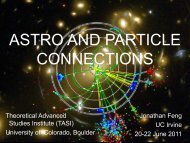
happen near the TeV scale. This is apparently possible with significant consequences for Higgsboson physics, as I shall now outline.Consider an expansion in H † H/M 2 , which is a SM singlet that can play the role of S.Immediately you may wonder how this is possible, since H † H cannot carry any U(1) quantumnumber. But think of SUSY at the TeV scale. H u H d can carry U(1) number, and when reducedto SM this expansion in terms of H † H is consistent. Consider the following mass matrices interms of the expansion parameterɛ = v M . (54)⎛h u 11ɛ 6 h u 12ɛ 4 h u 13ɛ 4 ⎞ ⎛h d 11ɛ 6 h d 12ɛ 6 h d 13ɛ 6 ⎞M u = ⎜⎝ h u 21ɛ 4 h u 22ɛ 2 h u 23ɛ 2⎟⎠ v, M d = ⎜⎝ h d 21ɛ 6 h d 22ɛ 4 h d 23ɛ 4⎟⎠ v . (55)h u 31ɛ 4 h u 32ɛ 2 h u 33h d 31ɛ 6 h d 32ɛ 4 h d 33ɛ 2These matrices give good fit to masses and mixings, as in the case of anomalous U(1) model.The Yukawa couplings of the physical quark fields are no longer proportional to the massmatrices. We obtain for the Yukawa couplings,⎛7h u 11ɛ 6 5h u 12ɛ 4 5h u 13ɛ 4 ⎞ ⎛7h d 11ɛ 6 7h d 12ɛ 6 7h d 13ɛ 6 ⎞Y u = ⎜⎝ 5h u 21ɛ 4 3h u 22ɛ 2 3h u 23ɛ 2⎟⎠ , Y d = ⎜⎝ 7h d 21ɛ 6 5h d 22ɛ 4 5h d 23ɛ 4⎟⎠ , (56)5h u 31ɛ 4 3h u 32ɛ 2 h u 337h d 31ɛ 6 5h d 32ɛ 4 3h d 33ɛ 2This leads to flavor changing Higgs processes, which however are within experimental limits.The branching ratios of the Higgs get modified, and is shown in Fig. 3.16

Q3Q3cd2,3(a)3u c d(b)_F F1 1HuHSQ2uc3(c)_G G G G1 1 2 2_HuSSQ3uc2(d)_G G G G3 3 4 4_HuSSQ 2cd 2,3(e)_ _ _F F F F FF22 3 3 1 1H dSSSQ 2u 2c(f)_ _ _ _G G G G G G G G1 1 2 2 3 3 4 4S SH SuSFigure 2: Frogatt–Nielsen fields generating Eq. (52).17

Figure 3: Higgs branching ratios with the SM Higgs as a flavon field.18