nistir 6921 - Building and Fire Research Laboratory - National ...

NISTIR 6921CONTAMW 2.0 User ManualMultizone Airflow and Contaminant Transport Analysis SoftwareW. Stuart DolsGeorge N. Walton

NISTIR 6921CONTAMW 2.0 User ManualMultizone Airflow and Contaminant Transport Analysis SoftwareW. Stuart DolsGeorge N. WaltonNovember 2002Building and Fire Research LaboratoryNational Institute of Standards and TechnologyU.S. Department of CommerceDonald L. Evans, SecretaryTechnology AdministrationPhillip J. Bond, Undersecretary of Commerce for TechnologyNational Institute of Standards and TechnologyArden L. Bement, Jr., Director

AbstractThis manual describes the computer program CONTAMW version 2.0 developed by NIST.CONTAMW is a multizone indoor air quality and ventilation analysis program designed to helpyou determine: airflows and pressures – infiltration, exfiltration, and room-to-room airflows andpressure differences in building systems driven by mechanical means, wind pressures acting onthe exterior of the building, and buoyancy effects induced by temperature differences betweenthe building and the outside; contaminant concentrations – the dispersal of airbornecontaminants transported by these airflows and transformed by a variety of processes includingchemical and radio-chemical transformation, adsorption and desorption to building materials,filtration, and deposition to building surfaces; and/or personal exposure – the prediction ofexposure of building occupants to airborne contaminants for eventual risk assessment.CONTAMW can be useful in a variety of applications. Its ability to calculate building airflowsand relative pressures between zones of the building is useful for assessing the adequacy ofventilation rates in a building, to determine the variation in ventilation rates over time, todetermine the distribution of ventilation air within a building, and to estimate the impact ofenvelope air tightening efforts on infiltration rates. The program has been used extensively forthe design and analysis of smoke management systems. The prediction of contaminantconcentrations can be used to determine the indoor air quality performance of buildings beforethey are constructed and occupied, to investigate the impacts of various design decisions relatedto ventilation system design and building material selection, to evaluate indoor air quality controltechnologies, and to assess the indoor air quality performance of existing buildings. Predictedcontaminant concentrations can also be used to estimate personal exposure based on occupancypatterns.Version 2.0 contains several new features including: non-trace contaminants, unlimited numberof contaminants, contaminant-related libraries, separate weather and ambient contaminant files,building controls, scheduled zone temperatures, improved solver to reduce simulation times andseveral user interface related features to improve usability.Key Words: airflow analysis; building controls; building technology; computer program;contaminant dispersal; controls; indoor air quality; multizone analysis; smoke control; smokemanagement; ventilationiii

DisclaimerThis software was developed at the National Institute of Standards and Technology byemployees of the Federal Government in the course of their official duties. Pursuant to title 17Section 105 of the United States Code this software is not subject to copyright protection and isin the public domain. CONTAMW is an experimental system. NIST assumes no responsibilitywhatsoever for its use by other parties, and makes no guarantees, expressed or implied, about itsquality, reliability, or any other characteristic. We would appreciate acknowledgement if thesoftware is used. This software can be redistributed and/or modified freely provided that anyderivative works bear some notice that they are derived from it, and any modified versions bearsome notice that they have been modified.Users are warned that CONTAMW is intended for use only by persons competent in the field ofairflow and contaminant dispersal in buildings and is intended only to supplement the judgmentof the qualified user. The computer program described in this report is a prototype methodologyfor computing the airflows and contaminant migration in a building. The calculations are basedupon a simplified model of the complexity of real buildings. These simplifications must beunderstood and considered by the user.Certain trade names and company products are mentioned in the text or identified in anillustration in order to adequately specify the equipment used. In no case does such anidentification imply recommendation or endorsement by the National Institute of Standards andTechnology, nor does it imply that the products are necessarily the best available for the purpose.iv

Table of ContentsAbstract......................................................................................................................... iiiDisclaimer ..................................................................................................................... iv1 Introduction.............................................................................................................. 11.1 What is CONTAMW? ...................................................................................................11.2 What's New in This Version? ........................................................................................11.3 System Requirements.....................................................................................................22 Getting Started......................................................................................................... 32.1 Installing CONTAMW ..................................................................................................32.2 Running CONTAMW....................................................................................................42.3 User Tasks......................................................................................................................42.4 The CONTAMW Graphical User Interface...................................................................62.5 Components of a CONTAMW Project..........................................................................83 Using CONTAMW................................................................................................... 123.1 Working with the SketchPad .......................................................................................123.2 Working with Project Files ..........................................................................................173.3 Configuring CONTAMW............................................................................................183.4 Working with Walls.....................................................................................................203.5 Working with Levels....................................................................................................223.6 Working with Zones ....................................................................................................243.7 Working with Airflow Paths........................................................................................273.8 Working with Simple Air Handling Systems ..............................................................463.9 Working with Ducts.....................................................................................................523.10 Working with Controls ................................................................................................643.11 Working with Species and Contaminants....................................................................733.12 Working with Sources and Sinks.................................................................................833.13 Working with Occupant Exposure...............................................................................903.14 Working with Data and Libraries ................................................................................933.15 Working with Weather and Wind................................................................................983.16 Working with Schedules............................................................................................1053.17 Working with Simulations .........................................................................................1093.18 Working with Simulation Results..............................................................................1173.19 Working with Project Annotations ............................................................................1263.20 Getting Help...............................................................................................................1274 Special Applications of CONTAMW ................................................................... 1284.1 Building Pressurization Test......................................................................................1284.2 Smoke Control Systems.............................................................................................1294.3 Shafts..........................................................................................................................1295 Theoretical Background...................................................................................... 1315.1 Model Assumptions ...................................................................................................1315.2 Contaminant Analysis................................................................................................1325.3 Airflow Analysis........................................................................................................1376 References ........................................................................................................... 155v

INTRODUCTION – WHAT IS CONTAMW?1 Introduction1.1 What is CONTAMW?CONTAMW is a multizone indoor air quality and ventilation analysis computer programdesigned to help you determine:(a) airflows: infiltration, exfiltration, and room-to-room airflows in building systems drivenby mechanical means, wind pressures acting on the exterior of the building, andbuoyancy effects induced by the indoor and outdoor air temperature difference.(b) contaminant concentrations: the dispersal of airborne contaminants transported by theseairflows; transformed by a variety of processes including chemical and radio-chemicaltransformation, adsorption and desorption to building materials, filtration, and depositionto building surfaces, etc.; and generated by a variety of source mechanisms, and/or(c) 0personal exposure: the predictions of exposure of occupants to airborne contaminantsfor eventual risk assessment.CONTAMW can be useful in a variety of applications. Its ability to calculate building airflows isuseful to assess the adequacy of ventilation rates in a building, to determine the variation inventilation rates over time and the distribution of ventilation air within a building, and toestimate the impact of envelope air tightening efforts on infiltration rates. The prediction ofcontaminant concentrations can be used to determine the indoor air quality performance of abuilding before it is constructed and occupied, to investigate the impacts of various designdecisions related to ventilation system design and building material selection, and to assess theindoor air quality performance of an existing building. Predicted contaminant concentrations canalso be used to estimate personal exposure based on occupancy patterns in the building beingstudied. Exposure estimates can be compared for different assumptions of ventilation rates andsource strengths.1.2 What's New in This Version?Throughout this manual you will find new features of the program highlighted in blue text asillustrated by this paragraph.CONTAMW 2.0 maintains the same features as CONTAMW 1.0 [Dols, Walton and Denton2000] with many enhancements - several of which are listed below. CONTAMW 2.0 isbackwards compatible with version 1.0 meaning you can open existing projects created withCONTAMW 1.0.Enhancements to CONTAMW 2.0• Building controls – Controls include sensors, actuators, modifiers and links. Controlactuators can be used to modify various characteristics of building components based oncontrol signals obtained from sensors and even modified by signal modifiers. For example, asensor can be used to obtain a contaminant concentration within a zone, and a proportionalcontrol actuator can be used to adjust supply airflow into the zone based on the sensedconcentration.1

INTRODUCTION – SYSTEM REQUIREMENTS• Scheduled zone temperatures – Zone temperatures can now be varied through the use of userdefinedschedules. This allows for the change in zone pressures due simply to the change intemperature within the zone according to the ideal gas relationship.• Contaminantso Non-trace contaminants – You can now account for the impact of contaminantconcentrations on the density of the air, e.g., water vapor.o Unlimited number of contaminants – CONTAM no longer restricts the number ofcontaminants you can simulate. The previous limitation was 10.o Contaminant-related libraries – Contaminant related elements can now be shared throughCONTAM library files. These elements include contaminant species, filters, source/sinksand kinetic reactions.• Numerical methodso Variable air density – CONTAMW now provides the ability to simulate non-flow relatedprocesses that can lead to the accumulation/reduction of mass within building zones, e.g.,due to non-trace contaminant sources and to variations in the zone pressure due to thechange in zone temperature.o Improved numerical solver implementing sparse matrix techniques to greatly reducetransient simulation times for large problems.o Separated solver from graphical user interface to provide for batch execution ofsimulations and directly utilize .PRJ files.• Transient weathero Separate transient weather and contaminant files – Weather files (.WTH) no longercontain contaminant concentrations (except for outdoor humidity ratio). This means youdon’t have to create different weather files depending on the types of contaminants youare simulating. CONTAM now provides you with the option of simulating transientambient contaminant concentrations using a contaminant file (.CTM).o Weather file creation/conversion software – NIST has developed a software tool thatallows you to convert existing weather files to CONTAMW 2.0 compatible weather files.You can convert your existing 1.0-compatible files, TMY2 and EnergyPlus weather files.• User interfaceo Longer zone names – Zone names can now be up to 31 characters long.o SketchPad zooming feature – You can now reduce the icon size of the SketchPad toallow the display of larger projects on the screen.o Display of net inter-zonal airflow results for highlighted zoneso Distinct simple air-handling system zones – The implicit zones of multiple simple airhandlingsystem are now distinguished from each other to allow for the plotting ofindividual system zones.o Airflow direction indicators are now displayed in the Status Bar when viewing airflowpath results.1.3 System RequirementsCONTAMW runs under Windows 95/98, NT/2000, and XP.2

GETTING STARTED – INSTALLING CONTAMW2 Getting Started2.1 Installing CONTAMW Obtaining CONTAMWCONTAMW installs from a set of installation files that you can obtain from NIST. These filescan either be downloaded from the NIST website (www.bfrl.nist.gov/IAQanalysis) directly ontoyour computer's hard disk, or you can obtain a set of floppy disks or CD that contains the setupfiles from the Indoor Air Quality and Ventilation Group (301) 975-6431. Installing CONTAMWIf you downloaded CONTAMW from the NIST website then you first double click the selfextractingarchive file "contamw2z.exe" to decompress the setup files. Extract the files to thesubdirectory of your choice, or simply select the default location. Once you have extracted thesetup files, you can run the setup program, "setup.exe." This will prompt you to perform anautomatic installation of the program. Read the directions to complete the installation.To install from a set of floppy disks or CD, insert the disk labeled "Disk 1" into the drive and runthe program, "setup.exe." This will prompt you to perform an automatic installation of theprogram. Follow the directions to complete the installation. Files InstalledThe following table lists the files installed by the setup program. For each file, the directory towhich it is installed, the name and a brief description are given. The directory is thatselected by you when you install the program. The default is C:\Program Files\CONTAMW2.The directory is that of the operating system fonts. The default is /FONTS,where depends on the operating system you are using, e.g., Windows 2000 = WINNT and Windows 95/98 = WINDOWS.Directory File Name Description contamw2.exe user interfacecontamx2.execontam.cfgcwhelp2.hlpcwhelp2.cntolch2d32.dllroboex32.dllSolverConfiguration filehelp filescharting and help displaydynamic link libraries\samples *.prj, *.wth and *.ctm sample project files*.lb?CONTAM library files walton##.fnt SketchPad fonts where ##ranges from 01 to 16 fordifferent SketchPadresolutions3

GETTING STARTED – RUNNING CONTAMW Uninstalling CONTAMWThe CONTAMW setup program will also provide you with an uninstall feature. You uninstallCONTAMW much as you would a typical Windows program. Access the Control Panel fromthe Settings selection of the Start menu. Select Add/Remove Programs from the Control Panel.Select CONTAMW from the list of installed programs and click the "Add/Remove…" button touninstall CONTAMW.2.2 Running CONTAMWAfter you install CONTAMW, you can run it by selecting CONTAMW from the NIST programgroup of the Start menu.2.3 User TasksThe use of CONTAMW to analyze airflow or contaminant migration in a building involves fivedistinct tasks:1. Building Idealization: Form an idealization or specific model of the building beingconsidered,2. Schematic Representation: Develop a schematic representation of the idealized buildingusing the CONTAMW SketchPad to draw the building components,3. Define Building Components: Collect and input data associated with each of the buildingcomponents represented on the SketchPad,4. Simulation: Select the type of analysis you wish to conduct, set simulation parameters,and execute the simulation,5. Review & Record Results: Review the results of your simulation and record selectedportions of the results.Task 1 - Building IdealizationBuilding idealization refers to the simplification of a building into a set of zones that arerelevant to the user’s goal in performing an analysis. A building can be idealized in a numberof ways depending on the building layout, the ventilation system configuration and theproblem of interest. This idealization phase of analysis requires some engineering knowledgeon the part of the user and is an acquired skill that you can develop through experience inairflow and indoor air quality analysis and by becoming familiar with the theoreticalprinciples and details upon which indoor air quality analysis is based.It is important to note that CONTAMW provides a macroscopic model of a building. In thismacroscopic view, each zone is considered to be well-mixed. Well-mixed means that a zoneis characterized by a discrete set of state variables, i.e., temperature, pressure andcontaminant concentrations. CONTAMW is well suited for analyzing the interaction betweenthe zones of a building on a macroscopic level but is not well suited for the analysis of themicroscopic airflow and contaminant characteristics within a given zone of a building.Computational Fluid Dynamics (CFD) analysis is better suited for analyzing the airflow andcontaminant transport characteristics of a given zone of a building. However, to date thecomputational resources required to perform a CFD analysis for an entire building isprohibitive.4

GETTING STARTED – USER TASKSTask 2 - SketchPad RepresentationDeveloping the SketchPad representation will be the focus of your interaction withCONTAMW. With CONTAMW's SketchPad you will be able to draw a diagram – aSketchPad diagram – of your building idealization using drawing tools and libraries of iconsto represent components of the building system. CONTAMW translates your diagram into asystem of equations that will than be used to model the behavior of the building when youperform a simulation.Task 3 - Data EntryData entry can be one of the more time-consuming parts of the process of usingCONTAMW. It involves the determination and input of the numerical values of theparameters associated with each of the SketchPad icons. These icons represent the elementsof the building model and include air leakage paths (windows, doors, cracks), ventilationsystem elements (fans, ducts, vents), contaminant sources, filters, and sinks and controlnetwork components. Each of these elements is associated with a number of parameters, andyou must obtain the values of these parameters for entry into the model. Depending on theelement and the application, these values can be obtained from building-specific data,engineering handbooks, and product literature. In many cases, a degree of engineeringjudgment will be involved. CONTAMW allows you to create libraries of these elements thatyou can use in current and future modeling efforts.Task 4 - SimulationSimulation is the use of CONTAMW to solve the system of equations assembled from yourSketchPad representation of a building to predict the airflow and contaminant concentrationsof interest. This step involves determining the type of analysis that is needed; steady- state,transient or cyclical, and a number of other simulation parameters. These parameters dependon the type of analysis you wish to perform (steady state or transient), and includeconvergence criteria and in the case of a transient analysis, time steps and the duration of theanalysis.Task 5 - Review & Record ResultsCONTAMW allows you to view the simulation results on the screen and to output them to afile for input to a spreadsheet program or a data analysis program developed by the user.Airflows and pressure differences at each flow element can be viewed directly on theSketchPad. Contaminant concentrations for a zone can also be plotted as a function of timedirectly from the SketchPad. You can then decide which data you wish to examine moreclosely and export these to a tab-delimited text file that can then be imported into aspreadsheet for further analysis.There is also a controls-related feature that provide the ability to report the values of userselectedcontrol nodes to a control "log" file for each time step of a transient simulation.5

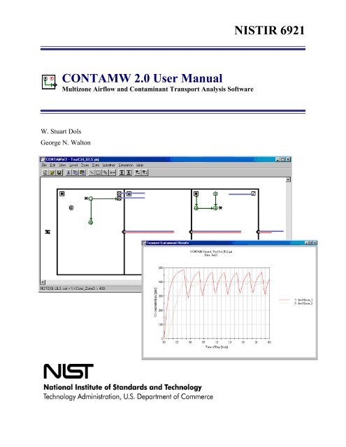
GETTING STARTED – THE CONTAMW GRAPHICAL USER INTERFACE2.4 The CONTAMW Graphical User InterfaceThe CONTAMW graphical user interface (GUI) is what you use to create and view your airflowand contaminant dispersal analysis projects. It consists mainly of a drawing region referred to asthe SketchPad, a set of drawing tools, a title bar, a set of menus, and a status bar. The followingsections provide brief explanations of each of the features of the CONTAMW GUI. See theUsing CONTAMW section for details on how to use these features.2.4.1 SketchPadFigure – The CONTAMW Graphical User InterfaceThe SketchPad is the region of the CONTAMW screen where you draw the schematicrepresentation of a building you wish to analyze. This representation is in the form of a set ofsimplified floor plans that represent the levels of a building. The SketchPad is used to establishthe geometric relationships of the relevant building features and is not intended to produce ascale drawing of a building. It should be used to create a simplified model where the walls,zones, and airflow paths are topologically similar to the actual building (See Working with theSketchPad).2.4.2 Title BarThe title bar is the typical rectangular region at the top of the main CONTAMW window. TheCONTAMW project filename will be displayed within this region.2.4.3 MenuThe menu is typical of a Windows program with differences that provide functionality specific tothe CONTAMW application. It is through this menu that most CONTAMW operations can beperformed including: saving and retrieving project files, selecting various modes of display,6

GETTING STARTED – THE CONTAMW GRAPHICAL USER INTERFACEsetting up and performing simulations, as well as accessing the on-line help system. Note thatsome of the menu items have shortcuts or hot-keys that enable quick access; for example, to savethe current project file use the Ctrl+S key combination.2.4.4 ToolbarThe toolbar, shown in the following figure, appears below the menu and provides convenientshortcuts to some of the menu items. Several of the toolbar buttons are similar to those found inother Windows applications. Other buttons provide a shortcut to functionality specific toCONTAMW.2.4.5 Status BarThe status bar, shown in the following figures, is the region displayed below the SketchPad at thebottom of the main window. This region is broken up into three separate panes that displayvarious information depending on the current mode of the SketchPad. Left PaneThis pane always displays the type and number of building component icon, e.g., zone, path, airhandling system, etc.In the normal mode of operation, the leftmost pane displays summary information of thecurrently highlighted cell or icon.In the simulation results mode, the leftmost pane displays the results for the currently highlightedicon. For a zone this includes the temperature and pressure relative to the ambient pressure at thebase of the building (see Wind Properties), for paths it will be the airflow and pressure dropacross the path along with symbols to indicate the direction of flow (>,

GETTING STARTED – COMPONENTS OF A CONTAMW PROJECT2.5 Components of a CONTAMW Project2.5.1 Project FilesAll data related to the characteristics of the projects you work with are stored in a "project" filehaving a "PRJ" extension (See Working with Project Files). This is an ASCII file, which isintended to be "viewed" only by the CONTAMW program. You should keep careful records ofyour project files and establish a naming convention that is meaningful to you for the variousversions of a project that you may wish to save.There are other files utilized by CONTAMW including: simulation results files, weather files,library files, and the log file. Simulation results are stored in files created automatically byCONTAMW with the same name as the PRJ file except that the "PRJ" extension is replaced bythe "SIM," "SUM" and "EXP" extensions depending on the type of results generated by thesimulation (see Working with Simulation Results). Weather files and contaminant files, typicallygiven the WTH and CTM extension, respectively, may contain up to a years worth of weatherand outdoor contaminant data and are used when performing transient simulations (see Workingwith Weather). Weather and contaminant files are ASCII files, but the data is of a format uniqueto CONTAMW. Library files are the means by which you can share various types of databetween CONTAMW projects. Each type of library data has a different extension: LB0(contaminants and source/sinks), LB1 (schedules), LB2 (wind pressure profiles), LB3 (airflowelements) or LB4 (duct flow elements). You create libraries of data using CONTAMW (seeWorking with Data and Libraries). The log file, "CONTAMW2.LOG," is created in the directoryin which the executable program resides each time you run the program. This file keeps track ofoperations that you perform during your session with CONTAMW and is a useful tool in theevent that you require technical support from the program developers when working with theprogram (see Getting Help).2.5.2 Building ComponentsBuilding components are the items that characterize the physical makeup of a building that youdefine using the CONTAMW graphical user interface. This section briefly describes thesecomponents.LevelsCONTAMW represents buildings in terms of multiple levels, accounting for thecommunication of air and contaminants between these levels. Levels typically correspond tofloors of a building, but a suspended ceiling acting as a return air plenum or a raised flooracting as a supply plenum may also be treated as a level.WallsWalls are used to designate zones which are regions surrounded by walls, floor and ceiling.These walls include the building envelope and internal partitions with a significant resistanceto airflow.Floors and CeilingsFloors and ceilings are included implicitly by CONTAMW for building zones. When youdraw a zone on the SketchPad, CONTAMW automatically includes the floor of the zone. Tocreate a roof with penetrations into the floor below requires a blank level above the top floor.8

GETTING STARTED – COMPONENTS OF A CONTAMW PROJECTIt is also possible to create a phantom zone with no floor or ceiling as might be required tocreate an atrium that spans multiple levels (see Working with Zones).ZonesA zone indicates a volume of air with uniform temperature and contaminant concentration.There are three types of zones in CONTAMW: normal, phantom and ambient. Normal zonesare separated from the zone below by a floor. The ambient zone, which surrounds thebuilding is implicitly defined and is identified by the symbol at the upper-left corner of theSketchPad. Any additional ambient zones must be connected to the default ambient zone. Forexample, you could use an ambient zone icon to define a courtyard. Phantom zones indicatethat the area on the current level is actually part of the zone on the level immediately below.There is no floor between a phantom zone and the zone below. You could use the phantomzone to define building features such as an atrium.Airflow PathsAn airflow path indicates some building feature by which air can move from one zone toanother. Such features include cracks in the building envelope, open doorways, and fans.Path symbols placed on the walls are used to represent openings between zones or toambient; any other placement represents an opening in the floor to the zone on the levelbelow. CONTAMW can implement several different models or airflow elements to defineairflow paths. The basic categories of airflow elements or models are as follows: small andlarge crack/openings represented by power-law and quadratic pressure relationships, smalland large doorways elements, and fan/forced airflow elements. (See Working with AirflowPaths)Simple Air-handling SystemsThe simple air-handling system (AHS) provides a simple means of introducing an airhandlingsystem into a building without having to draw a duct system. It provides areasonable model of an air-handling system that delivers user-specified flows where thesystem is properly balanced and the fan is not impacted by any other pressurizing effects inthe building. The AHS consists of two implicit airflow nodes (return and supply), threeimplicit flow paths (recirculation, outdoor, and exhaust air), and multiple supply and returnpoints that you place within the zones of the building. You can set the air flows of the AHSto vary according to a schedule.DuctsYou can use ducts to implement a more detailed model of an air-handling system thathandles a broader range of conditions. For example, when an air handler is off, the ductworkmay provide flow paths between zones which are significant in relation to the normalconstruction cracks or openings. Ductwork consists of duct segments (paths) and junctions orterminal points (nodes). CONTAMW can implement several different duct segment modelsor duct flow elements to define duct segments. The basic categories of duct flow elements areas follows: resistance models, fan performance curves, and back-draft dampers. (SeeWorking with Ducts)9

GETTING STARTED – COMPONENTS OF A CONTAMW PROJECTContaminants, Sources and SinksYou can define an unlimited number of contaminants within a single project with apractically limitless number of sources associated with the contaminants. CONTAMW cansimulate contaminant transport via airflow between zones, removal by filtration mechanismsassociated with flow paths, and removal and addition by chemical reaction. CONTAMW canalso implement several source and sink models to generate contaminants within or removecontaminants from a zone. These models include: constant generation, pressure driven,decaying source, cutoff concentration, reversible boundary layer diffusion, and burst models.(See Working with Contaminants and Working with Sources and Sinks)SchedulesSchedules are used to control or modify various properties of building components as afunction of time. You can set schedules for airflow paths, duct flow paths; contaminantsources and sinks; and inlets, outlets and outdoor air delivery of simple air-handling systems.The effect of setting a schedule on a building component varies depending on the propertiesof the component. For example, you can set a schedule to adjust the airflow delivered to azone by an inlet of a simple air-handling system. (See Working with Simple Air HandlingSystems)CONTAMW 2.0 provides the ability to schedule zone temperatures.ControlsControls include sensors, actuators, modifiers and links. Control actuators can be used tomodify various characteristics of building components based on control signals obtainedfrom sensors and even modified by signal modifiers. For example, a sensor can be used toobtain a contaminant concentration within a zone, and a proportional control actuator can beused to adjust supply airflow into the zone based on the sensed concentration.2.5.3 OccupantsOccupants can be used to determine the amount of contaminant exposure a person would besubjected to within a building. Occupants can also generate contaminants. You can set a scheduleto establish each occupant’s movement within a building. Occupant schedules can also be usedto define periods of times when occupants are not in the building. (See Working with OccupantExposure)2.5.4 WeatherCONTAMW enables you to account for either steady-state or varying weather conditions.Weather conditions consist of ambient temperature, barometric pressure, humidity ratio, windspeed and direction, as well as ambient contaminant concentrations.2.5.5 Wind Pressure ProfilesWind pressure profiles are used to describe the wind direction effects on the envelope of abuilding. Wind pressure profiles simplify the somewhat difficult process of accounting for thefact that the facades of a building envelope are affected differently depending on their orientationrelative to the wind.10

GETTING STARTED – COMPONENTS OF A CONTAMW PROJECT2.5.6 SimulationIn CONTAMW, simulation is the process of forming a set of simultaneous equations based uponthe information stored in the project file, performing the numerical analysis to solve the set ofnodal equations according to user-defined specifications, and creating simulation results files thatcan be viewed using the CONTAMW interface. There are three basic types of simulations thatyou can perform for airflow and contaminant analysis using CONTAMW: steady state, transientand cyclical. (see Working with Simulations)11

USING CONTAMW – WORKING WITH THE SKETCHPAD3 Using CONTAMWThis section provides detailed information on how to use the features of the CONTAMWapplication as well as a detailed explanations of the terminology of the user interface. Youshould think of this section as your detailed conceptual and contextual guide to working with theCONTAMW program.3.1 Working with the SketchPadThe SketchPad is the region of the CONTAMW screen where you draw the schematicrepresentation of a building you wish to analyze. This representation is in the form of a set ofsimplified floor plans that represent the levels of a building. The SketchPad consists of aninvisible array of cells into which you place various icons to form your schematics of a building.The SketchPad is used to establish the geometric relationships of the relevant building featuresand is not intended to produce a scale drawing of a building. It should be used to create asimplified model where the walls, zones, and airflow paths are topologically similar to the actualbuilding.When working with CONTAMW you will notice a blinking square on the SketchPad. This isknown as the system caret, and it is the size of a single SketchPad cell. This caret is the samething as the blinking vertical bar that is common to many word processing applications. Thecaret indicates the currently selected cell of the SketchPad. Any icon-related information thatappears in the status bar is associated with the location of the caret. To move the caret around theSketchPad you can use the keyboard arrow keys or you can move the system cursor with themouse and click the left mouse button to set the caret position.The specific operations that you will perform using the SketchPad are as follows:1. Drawing Walls, Ducts and Controls2. Drawing building component icons3. Defining building component icons4. Viewing results5. Viewing envelope pressure differentials due to wind effectsSketchPad ModesThere are three modes of the SketchPad: normal, results and wind pressure. The SketchPadmode basically refers to the type of information that is displayed upon the SketchPad. Youcan tell what mode the program is in by looking at the items in the View menu to see whichones are checked.In the normal mode CONTAMW displays only the building component icons. In this modeyou can add, delete, copy, and move icons.In the results mode, CONTAMW displays simulation results upon the SketchPad. In thismode you will not be allowed to add, delete, copy and move icons upon the SketchPad (SeeViewing Results).The wind pressure mode is provided to verify wind speed and direction information visuallyon the SketchPad. (See CheckingWind)12

USING CONTAMW – WORKING WITH THE SKETCHPADPrinting SketchPad ImagesYou can obtain images of your SketchPad drawings to print or edit using the Windows printscreen feature. To do this, size the CONTAMW window and press Alt+PrintScrn on thekeyboard to copy the current window to the Windows clipboard. Then you can immediatelypaste the image into the desired program. For example, you can paste the image into theWindows Paint program for editing or directly into a word processing program. You can thenprint the image from either of these programs.Exporting .PCX SketchPad FilesYou can save a SketchPad image of the currently displayed level to a .PCX graphics fileusing the File → Save SketchPad to .PCX File… menu item. The Save As dialog box willappear allowing you to name the file. The file will contain a black and white image made upof 8 by 8 pixel icons.3.1.1 Drawing Walls, Ducts and ControlsYou use various tools to draw the physical features of the building such as walls and ducts. Alldrawing can be accomplished with either the mouse or the keyboard. When drawing, thefollowing mouse and keyboard keys produce common behavior. The left mouse button (LMB)corresponds to the ↵, or Enter key; the right mouse button (RMB) to the Esc key. Verticalmotion of the cursor corresponds to the ↑ and ↓ cursor keys, and horizontal motion correspondsto the ← and → cursor keys.The basic steps for drawing walls and ducts are as follows:1. Activate drawing tool,2. Set the initial location of the object,3. Draw the object,4. Undo current drawing,5. Finalize drawing the object, and6. Deactivate drawing tool. Activating a Drawing ToolThere are four drawing tools available, two for drawing walls, one for drawing ducts and one fordrawing control networks. To activate a drawing tool either select it from the toolbar, select itfrom the "Tools" menu, or use the shortcut associated with the menu item. The toolbar button ofa selected drawing tool will remain depressed as long as that tool is active. The toolbar buttonsand associated menu shortcuts are shown here.rectangle (or box) drawing tool (Ctrl+B)free-form wall drawing tool (Ctrl+W)duct drawing tool (Ctrl+D)controls drawing tool (Ctrl+L)13

USING CONTAMW – WORKING WITH THE SKETCHPADOnce you have selected the tool, the drawing cursor will be displayed. The drawing cursor is apink square the size of a single SketchPad cell. Initially, the cursor appears with a transparentcenter. Setting the Initial Location of the ObjectTo begin drawing the object, you set the initial location by first moving the drawing cursor eitherwith the mouse or the keyboard arrow keys and then you either click the LMB or press ↵ on thekeyboard. This will anchor the beginning of the object at the nearest valid SketchPad cell for thetype of object you are drawing. When you select a valid beginning location, the drawing cursorwill become solid and you can begin drawing your object. Drawing the ObjectAfter you anchor the beginning of the object, you simply use the mouse and/or keyboard arrowkeys to draw the desired shape. While you are drawing, the cursor will be restricted to theSketchPad region and constrained to specific movements in order to maintain drawing withinvalid cells of the SketchPad. As you move the cursor, a dark line will appear on the SketchPadrepresenting the shape of the object you are drawing. Undoing the Current DrawingPrior to finalizing the drawing of the object, you can undo your drawing. To undo what you havedrawn, either single-click the RMB or press the Esc key. This will erase the thick dark line, butyou will still be in the drawing mode. To begin drawing again, set the initial location again andcontinue drawing another object. Finalizing the Drawing ObjectOnce you are satisfied with your drawing, you finalize the object by either single-clicking theLMB or pressing the ↵ key. This will replace the cells that had the thick dark line with the iconsappropriate for completing the type of object you are drawing. If you have attempted to draw aninvalid object, you will be prompted with a dialog box containing a message indicating the typeof error, and then you will be allowed to repair the drawn object. Deactivating Drawing ToolsWhen you are finished using a drawing tool you click the RMB or press Esc until your systemcursor reappears. Also, selecting a different drawing tool will automatically deactivate thecurrent tool if you do not currently have an object anchored.3.1.2 Drawing Building Component IconsA set of icons is used to represent various building components such as airflow paths(representing doors, windows, cracks, etc.), contaminant sources and sinks, occupants and airhandlingsystems. You place icons on the SketchPad using the Right Mouse Button to displaya pop-up menu and then selecting the desired building component from the menu.This icon placement menu is context-sensitive. The menu selections that you can choose fromthe icon placement menu will depend on the contents of the cell occupied by the caret andwhether the SketchPad is currently displaying simulation results. When results are beingdisplayed, you will not be allowed to place additional icons on or delete icons from theSketchPad. This is done to prevent the display of misleading results on the SketchPad due to a14

USING CONTAMW – WORKING WITH THE SKETCHPADmismatch in the number of icons on the SketchPad and the number of icons for which results areavailable from the last simulations. The icon placement menu will also prevent you from placingicons on invalid SketchPad locations. For example, you cannot place a supply or return of asimple air-handling system within the ambient zone.The following figure shows the pop-up icon placement menu.The following table is a list of the icons that you will see on the CONTAMW SketchPad. Thislist shows the icons by categories of building components. Some of these icons are placed on theIcon CategoryComponent IconsWallsZonesDuct SegmentsDuct JunctionsDuct TerminalsSimple AHSAirflow PathsSource/SinksOccupantsControls15

USING CONTAMW – WORKING WITH THE SKETCHPADSketchPad using the drawing tools, and others are placed using the pop-up icon placement menu.3.1.3 Defining Building Component IconsWhen a new building component icon is drawn upon the SketchPad, it appears as a red icon. Thecolor red indicates that the parameters of the component must still be defined. To define abuilding component, you double-click (LMB) on the icon or move the caret (represented by ablack square) to the icon and press the Enter key. This will activate the associated dialog box orproperty sheet for the selected component, into which you enter the parameters that define thecomponent. After you have entered the parameters of the component, click the OK button toaccept the parameters or the Cancel button not to accept the parameters. The detailed propertiesof each component icon will be presented throughout the "Using CONTAMW" section of thismanual. You can also access detailed descriptions of the component properties by pressing theF1 key (Help) while running the CONTAMW application.3.1.4 Deleting Building Component IconsTo delete undefined building component icons, you highlight the icon then delete it. Youhighlight the icon by either clicking (LMB) on the icon or moving the caret (represented by ablack square) to the icon using the arrow keys. You delete the highlighted icon by either pressingthe Delete key or using the menu command: Edit → Delete.3.1.5 Viewing Results on the SketchPadCONTAMW provides some graphical displays of simulation results upon the SketchPad. Youcan display airflow rates and pressure differences across airflow paths on the SketchPad if asimulation has been performed and results of the simulation are available (see Viewing Resultsin the Working with Results section of the manual).3.1.6 Viewing Envelope Wind Pressure DifferentialsCONTAMW provides a feature that allows you to visualize the effects of wind upon a buildingenvelope. A graphical display of wind pressures at each of the flow paths that are adjacent to theambient zone can be viewed on the SketchPad (see Checking Wind Pressure Data in theDefining Steady State Weather and Wind section). This feature enables you to verify input ofwind speed and direction data with respect to the orientation of the building envelope to thewind.16

USING CONTAMW – WORKING WITH PROJECT FILES3.2 Working with Project FilesAll information related to the layout, building components, and occupant information of yourCONTAMW project are stored in a "project" file. When you save the project file, it will bestored with the ".PRJ" extension. CONTAMW project file names must conform to the filenaming conventions of the Windows operating system. This project name is displayed in theTitle bar of the CONTAMW application window.All project file operations are contained under the File menu. These operations include: NewProject, Open Project…, Save Project, and Save Project As… Note that some of these fileoperations have keyboard short-cuts and/or tool bar buttons associated with them. Creating a New ProjectMenu Command: File → New ProjectKeyboard Shortcut: NoneToolbar Button:Use this command if you are currently working on a project and you wish to create a new one.This command will clear the SketchPad and all data related to the current project fromCONTAMW's program memory. If your current project has been not been saved prior toexecuting this command, you will be asked whether or not you wish to save it prior to clearing it. Opening an Existing ProjectMenu Command: File → Open Project…Keyboard Shortcut: Ctrl+OToolbar Button:Use the menu item to open and existing CONTAMW project file. This command will display theFile Open dialog box typical of Windows applications. This dialog box is set to display onlythose files having the ".PRJ" extension in order to simplify your search for CONTAMW projectfiles. Follow the typical procedure for opening a file using the Windows operating system. Converting Projects from CONTAMW 1.0 to CONTAMW 2.0Menu Command: File → Open Project…Keyboard Shortcut: Ctrl+OThis is the same as opening an existing project. However, after you open a 1.0 formatted projectit will be untitled, so you must give the project a name when saving it. Once you save a projectwith the 2.0 format, you will no longer be able to open it using 1.0. Saving a ProjectMenu Command:Keyboard Shortcut:Toolbar Button:File → Save ProjectCtrl+SThis option saves the building description to the project file under its current name. Wheneverthe project file is saved, the current version of the file is copied to CONTAM.BKP before arevised project file is written. You may be able to use this file to restore a project file in the eventthat it becomes corrupted.17

USING CONTAMW – CONFIGURING CONTAMW Renaming a ProjectMenu Command: File → Save Project As…Keyboard Shortcut: NoneToolbar Button: NoneUse this command to save a copy of the current project file under a new name. This will displaythe Windows "Save As" dialog box and allow you to specify both a storage location and a filename for the project file. CONTAMW will automatically append the ".prj" extension to thefilename, so you do not have to give the file an extension. If you do give the file an extension,".prj" will be appended as well as the extension you provide. If you specify the name of anexisting file, you will be warned that saving the file will overwrite the existing file. If you try tosave an untitled or new project file prior to giving it a name, the "Save As" dialog box will bedisplayed. Exiting CONTAMWMenu Command: File → ExitKeyboard Shortcut: NoneToolbar Button: NoneYou can also exit the program using the standard window-closing button located in the upperright-hand corner of the program window.3.3 Configuring CONTAMWThe project configuration settings of CONTAMW are available from the Options… selection ofthe View menu. This set of configuration properties will allow you to select the overall size ofthe SketchPad (i.e. the number cells that make up the height and width), the size of a singleSketchPad cell, the default system of units (SI or IP), the default units of mass flow and thedefault zone temperature. All of these settings are saved with the CONTAMW project with theexception of the cell size that resets back to the default size whenever you exit CONTAMW.You can also save the default units and values and the available cell sizes to a configuration file,CONTAM.CFG. CONTAMW looks for this file when starting and loads the saved settings if thefile exists. This way you can set CONTAMW to start with the same default settings each timeyou run the program.The following sections provide detailed descriptions of the specific configuration properties.They are the context-sensitive help topics that you can access by pressing F1 when working withproperty pages of the "Project Configuration Properties" property sheet.3.3.1 Default UnitsThe following parameters define the units and selected values that will be used by defaultthroughout the project when you are providing input to the program. You do not have to usethese units throughout the project; however, you should select the primary set of units forconvenience when entering data throughout a project. You can change these defaults at any timewhile working with a project, and you can select different units for individual parameters as youenter them.18

USING CONTAMW – CONFIGURING CONTAMWDefault System of Units: You can select the appropriate radio button to set the system of unitsthat you would like the program to use. You can either select the International System of Units(SI) or the Inch-Pound (IP) system of units.Default Units of Flow: You can select the appropriate radio button for the most commonly usedunits of flow in the current project. These are the units in which airflow simulation results will bedisplayed within the status bar. CONTAMW converts all airflow rates to and performs allcalculations in mass flow units of kg/s. Note that all volumetric airflow rate units are at standardtemperature and pressure.Default Zone Temperature: This value will be the default temperature used whenever youcreate a new zone within the current project.3.3.2 SketchPad SizeSketchpad Size (cells): This is the height and width of the SketchPad. The units (cells) representeach space where an icon may be placed upon the SketchPad. The default (and minimum) valuesare 66 cells wide and 58 cells high.Shift Drawing (cells): If you need more space on one side of a drawing you can shift the entireproject on the SketchPad. You may need to increase the size of the SketchPad to make room forthe project before shifting it. Entering a positive number in the "Horizontally" edit box will shiftthe project to the right relative to the SketchPad, and entering a positive number in the"Vertically" edit box will move the project down relative to the SketchPad. A negative numberwill have the opposite effect.3.3.3 Cell/Icon SizeCurrent Cell/Icon Size: There are seven options for displaying icons on the SketchPad (1x1,2x2, 3x3, 4x4, 5x5, 8x8, and 16x16). The default option is 8x8. This is a "zooming" feature thatprovides a visual aid to enable you to view sketches in more detail or to fit larger sketches withinthe program window. The cell size has no effect on the project simulation. There are two"zooming" buttons provided on the toolbar to quickly increase and decrease the cell sizeaccording to the available cell sizes below.Available Cell Sizes: Use these check boxes to select which sizes you want available. The 1x1size causes problems with some versions of the Window 98 operating system. If this is the casefor you, then deselect the 1x1 check box and click the "Save Configuration" button.19

USING CONTAMW – WORKING WITH WALLS3.4 Working with WallsIn CONTAMW, walls separate regions of uniform air temperature and contaminantconcentration on a given level. Walls include the building envelope and internal partitions with asignificant resistance to airflow. The enclosed regions you create within walls are known aszones. You will note when drawing on the SketchPad that you can only draw walls in oddnumbered rows and columns. This is done to avoid conflicts with ducts that can only be drawnon the even rows and columns of the SketchPad.It is important to realize that CONTAMW is not meant to provide drawing capabilities similar tothat of a Computer Aided Drawing (CAD) program. The SketchPad drawing functions weredesigned to provide a strict environment for creating the input to the underlying multizone modelupon which the CONTAMW simulation engine is based.3.4.1 Drawing WallsYou can draw walls using either of the two wall drawing tools previously described in the"Working with the SketchPad" section. Use the box drawing tool to quickly draw a rectangularregion and the wall drawing tool to draw a free form wall. Use the wall drawing tool to drawalmost any shape wall. Walls must always form complete enclosures. Therefore, a wall cannothave an open or dangling end. It also may not be drawn across building component icons. Youwill receive a warning message if you attempt to draw an invalid wall.3.4.2 Deleting WallsYou can delete a wall by moving the caret to any portion of the wall and selecting Delete fromthe Edit menu or using the keyboard shortcut Del key. CONTAMW will highlight the section ofwall to be deleted and request confirmation to delete the indicated section. If the caret is on theintersection of three or more walls, you will be given multiple options of wall segments to delete.If you select "No" when asked to confirm deletion, the next option for deletion will becomehighlighted until you either delete a section or all of the options are exhausted.20

USING CONTAMW – WORKING WITH WALLS3.4.3 Modifying WallsYou modify the positions or shapes of walls by adding and deleting wall sections. For examplein the following figures, if you want to modify the zone in figure (a) to obtain the zone in figure(d), you would first add the dark line in figure (b) then delete the dark line in figure (c).When modifying walls you may need to move or delete other icons. For example in thefollowing figures, to create drawing (c) from drawing (a), you would delete the lighter line andthe lighter zone icon from figure (b). You must delete one of the two zone icons, or you will endup with two zone icons within the same enclosed wall area. This is not permitted, and you willreceive a message indicating a zone definition error.21

USING CONTAMW – WORKING WITH LEVELS3.5 Working with LevelsCONTAMW projects are organized by levels. Each level of a CONTAMW project contains aplan view drawing. Typically, each level of a CONTAMW project corresponds to a floor of abuilding. Depending on the detail required for your modeling purposes, you could represent abuilding floor using multiple CONTAMW layers. For example, a level could be used torepresent a ceiling or floor plenum.3.5.1 Creating LevelsWhen you first start CONTAMW, a default level is created so that you can begin working on adrawing right away without having to create a new level. There are three commands in the Levelmenu that you use when creating new levels. These are the Copy Level, Paste Level, and InsertBlank Level commands. Whenever you create a new level, whether it is blank or a copy ofanother level, CONTAMW will give it a default name that will consist of a number enclosedwithin the "" characters. You can modify this name later by editing the data associatedwith a level.You must be careful when copying levels within CONTAMW. For example, you might have anair handler defined within a duct system on a level and then copy it to another level. This wouldcreate another air handler on the new level. If the ductwork is connected between the two levels,the two air handlers may act against each other. You must be careful to make connectionsbetween building levels in a manner that makes sense for your purposes. Creating Blank LevelsMenu Command: Level → Insert Blank Level (Above/Below Current Level)Keyboard Shortcut: NoneToolbar Button: NoneUse these commands to create a blank level. When you create a blank level, you must selectwhether you want it created above or below the current level. Copying and Pasting levelsMenu Command: Level → Copy Level along withLevel → Paste Level (Above/Below Current Level)Keyboard Shortcut: NoneToolbar Button: NoneWith CONTAMW you can copy an entire level and insert it as an entire level anywhere withinthe current project. Use the Copy Level command to copy the level currently displayed on theSketchPad; move to either the level above or below where you wish to insert the copied level anduse one of the Paste Level commands to insert the copied level.3.5.2 Viewing LevelsIf a project has more than one level, you can specify the level that you want to view or modify onthe SketchPad by using the level commands. All level-related commands are located under theLevel menu. There are also some shortcut keys and toolbar buttons provided for yourconvenience.22

USING CONTAMW – WORKING WITH LEVELS Changing the Currently Active LevelMenu Command: Level → Go to (Level Above/Below)Keyboard Shortcut: Page Up, Page DownToolbar Button:Use this command to change which level you want the SketchPad to display. Displaying Multiple LevelsMenu Command: Level → Reveal Level BelowKeyboard Shortcut: Ctrl+Shift+BToolbar Button: NoneUse this command to see both the current level and the level below the current level at the sametime. CONTAMW will displays the walls and building component icons of the level below ingray. This feature is useful for aligning building features between adjacent levels.3.5.3 Deleting LevelsMenu Command:Keyboard Shortcut:Toolbar Button:Level → Delete LevelNoneNoneUse this command to delete an entire level. Once you have deleted a level, you cannot undo thedeletion. You may want to save a copy of the file prior to deleting a level; this is the only way toprevent losing your work.3.5.4 Modifying LevelsTo modify level data, you access the Level Data dialog box using the Edit Level Data…command of the Level menu. You can also use the keyboard shortcut F8 to display the dialogbox. The following section shows the information contained on the "Level Data" dialog box.3.5.5 Level DataThis is the information associated with each level that you create. CONTAMW will providedefault values for this data, but you can modify it as required for your particular building.Name: Name to identify the level. All level names must be unique.Elevation of this level: The elevation of the base of the level above ground.Distance to level above: This is the height of the level from floor to ceiling. CONTAMW willuse this value to calculate zone volumes based on the floor area of each zone.3.5.6 Checking LevelsMenu Command:Keyboard Shortcut:Toolbar Button:Level → Check Current LevelNoneNoneUse this feature to check the data for the currently displayed level and make sure the buildingcomponents are defined. Errors will be highlighted in red.23

USING CONTAMW – WORKING WITH ZONES3.6 Working with ZonesA zone is a volume of air with uniform temperature and contaminant concentration. There arethree different types of zones: normal, phantom and ambient. A normal zone icon represents azone that is separated by a floor from the zone below. A phantom zone is used to indicate thatthere is no floor below the enclosed region on a given level. That is, the region on this level isactually part of the zone below and has the same temperature and contaminant concentration. Anambient zone icon represents the outdoor air. The ambient zone, which surrounds the building, isalready identified by default by the icon at the upper-left corner of the SketchPad.You create zones on the SketchPad by first drawing walls that enclose a region, placing a singlezone icon within the enclosed region, and then defining the zone icon. Eventually, every zonemust be connected to either the ambient zone or a constant pressure zone either directly orindirectly via any set of paths that prevents the zone from being isolated from a zone of "known"pressure.3.6.1 Creating ZonesYou create zones by drawing walls upon the SketchPad. The wall drawing operations aredescribed in the Drawing Walls section of this manual. The shape and size of zones as drawnupon the SketchPad do not provide the underlying model with any scaling information.However, the manner in which the enclosed regions border each other is significant. Any zonesbetween which you wish to provide a direct connection (via an airflow path) must share acommon wall. Therefore, when drawing a building floor plan, you should try to maintain thegeneral topology of the actual floor plan. While scale is not significant, CONTAMW doesprovide you with the SketchPad coordinates that may help you when laying out your project.The dimensions of your zones are determined when you define them. If you change the shape orsize of a region on the SketchPad that contains a zone icon, the dimensions do not changeaccording to the model unless you actually modify the properties of the associated zone icon.3.6.2 Deleting ZonesYou delete a zone by first deleting the zone icon. After you delete the zone icon, delete the wallor walls necessary to eliminate the enclosed region that is left behind. You must avoid theexistence of an enclosed region without a zone icon; CONTAMW will not perform a simulationwith an undefined zone icon in a project.3.6.3 Modifying ZonesYou modify the SketchPad representation of a zone by adding and removing walls. Thisprocedure is described in the Modifying Walls section of this manual. To modify the parametersof a zone, you use the icon definition procedure (See Defining Building Component Icons) todisplay its properties and make the desired changes.Once you define a zone, you can move the zone icon anywhere within the zone using the Cutand Paste functions of the Edit menu. These commands will only allow you to paste the iconinto the zone in which it is currently located.24

USING CONTAMW – WORKING WITH ZONES3.6.4 Defining ZonesAfter you draw the enclosed region of a zone, you must define the zone. To define a zone youmust first draw a zone icon within the enclosed region (See Drawing Building Component Icons)and then use the icon definition procedure (See Defining Building Component Icons) to displayand edit the properties of the zone.The properties of each zone include a name, temperature (constant or scheduled), pressure,volume and information describing contaminant behavior within the zone. You must provideeach zone with a name that is unique to each level of a project. For this reason, you cannot copyzone data within a level. However, you can copy entire levels of data, including zone data, fromone level to another (See Creating Levels). Detailed descriptions of zone properties are givenunder Zone Properties below.Only normal zones require definition. Ambient and phantom zone icons appear as defined iconsas soon as you place them onto the SketchPad. However, you must include the volume ofphantom zones in the volume of the associated normal zone below it.3.6.4.1 Zone PropertiesThis section provides detailed descriptions of the specific zone properties. The followingsections are the context-sensitive help topics that you can access by pressing F1 when workingwith property pages of the "Zone Properties" property sheet.Zone – Zone Data PropertiesThese are the basic properties that describe a zone.Zone Name: This is the symbolic name of the zone. Enter a name up to 15 characters in length.Zone names must be unique within each level of a building.DimensionsVolume: Zone volume is used in the dynamic contaminant calculations. For phantom zones,the zone volume is set at the standard zone icon on the lowest level for the entire height ofthe zone and includes the volume of the phantom zones on the levels above.Floor Area: Instead of the volume, you may enter a floor area. Floor area is then multipliedby the height of the current building level to compute a volume. This area is not used for anyother purpose by CONTAMW.TemperatureConstant or Scheduled: Select to either maintain zone temperatures at a constant value orto change according to a user-defined schedule. If you select Scheduled, then you mustassociate a temperature schedule with the zone. Selecting Scheduled will also set thesimulation run control to vary the density within building zones during simulation (SeeAirflow Numerics Properties in the Working with Simulations section).Temperature: Set the value you want CONTAMW to use as the constant temperature of thezone when you select the "Constant" radio button. Whenever you create a new zone,CONTAMW use the default value which you can override by entering another value. Youcan set the default zone temperature via the Options… command of the View menu.25

USING CONTAMW – WORKING WITH ZONESTemperature Schedule: Select the temperature schedule you want to associate with thiszone when you select the "Scheduled" radio button. (See Working with Schedules).Pressure: The zone air pressure relative to ambient can be specified as either variable orconstant. Typically you would set the zone pressure to be variable and let CONTAMWdetermine it. However, you might set the pressure to be constant if you want to simulate a fanpressurization (blower door) test of a building (see Building Pressurization Test in theApplications section of the manual) or to perform analytic test cases of CONTAMW.Zone – Contaminant PropertiesThese are the contaminant-related properties of a zone. Contaminants must be defined prior todefining contaminant data for a zone. To define contaminants, select Data then Contaminants…from the main program menu.Zone Name: This is the symbolic name of the zone as entered on the Zone Data property page.Contaminant Concentrations: Select variable or constant. Typically you would set this tovariable and allow CONTAMW to calculate the contaminant concentration within the zone.However, you may wish to set this to constant as a simple means of creating a simplecontaminant source within a zone. If you set this to constant, the contaminant concentrations inthis zone will begin and remain at the values you set for the initial concentrations.Initial Concentration: Select a contaminant from the list and enter the initial contaminantconcentrations for dynamic (transient) simulations. Note that only those species you’ve selectedto be contaminants (use in simulation) appear in the list. If a species for which you wish to set aninitial concentration does not appear in the list you must set "Use in simulation" property of thecorresponding species to be true (See Creating Species and Contaminants). You can reset theseinitial values through the Run Control Properties of the Simulation Parameters.IMPORTANT: Changing the number of contaminants, i.e. those species used in the simulation,will reset the initial concentrations of all zones to the default contaminant concentrations. Youcan reset all of these concentrations via the Run Control Properties as indicated above orindividually here.Kinetic Reactions: If there are previously defined kinetic reactions within the current project,you may select one from the list of names. Click the "New Reaction" button to define a newkinetic reaction. To view or modify existing kinetic reaction data click the "Edit Reaction"button. Setting this field to indicates no reactions in the zone. You can also importkinetic reactions from a contaminant-related library file (See Working with Data and Libraries).26

USING CONTAMW – WORKING WITH AIRFLOW PATHS3.7 Working with Airflow PathsAn airflow path is a CONTAMW building component through which air can move between twoadjacent zones. These components can be cracks in the building envelope, open doorways,exhaust fans, etc. The air pressures in the adjacent zones and the flow characteristics of the flowpath itself determine the flow through most of these paths. The location of the SketchPad iconthat represents a flow path determines the two zones that are connected by a flow path. If thepath icon is placed on a wall, it connects the zones on opposite sides of the wall. If it is placed ina blank cell of a zone (i.e. on the floor), it connects the zone containing the flow path icon to thezone located directly below the flow path icon.You can place airflow paths on the SketchPad, define their flow characteristics, move, copy, anddelete them. You must provide each airflow path with specific information that describes its flowcharacteristics. Much of the information that describes the flow characteristics of airflow paths iscontained in airflow elements that you must create when defining the airflow paths. The detailsof drawing, defining and modifying airflow paths are described in the following sections.3.7.1 Airflow ElementsEach airflow path must refer to an airflow element. Airflow elements describe the mathematicalrelationship between the flow through an airflow path and the pressure drop across the path.CONTAMW provides you with several mathematical models or types to choose from. Each ofthese airflow element types is described in detail in the Airflow Path Properties section. Whileevery airflow path must refer to a single airflow element, multiple paths can refer to the sameairflow element. Airflow elements can also be stored within a CONTAMW library file and sharedbetween different CONTAMW project files (See Working with Data and Libraries).3.7.2 Creating Airflow PathsYou create airflow paths by placing an airflow path icon on the SketchPad (See DrawingBuilding Component Icons). Because flow paths connect only two adjacent zones, there areseveral restrictions on the placement of flow paths. You may not place airflow path icons on thecorner of a zone or on the blank cell of a level that does not have a zone located directly below it.Note that you can place an airflow path icon on the "roof" of a building that connects a zonebelow to the ambient. In this case, the roof level would be a level that does not contain walls butcontains airflow path icons located in the floor of the roof level (above zones on the level below).The context-sensitive feature of the pop-up icon placement menu enforces these restrictions. The"Flow Path" menu selection will be disabled (grayed out) if you pop-up on a location whereCONTAMW does not allow the icon to be placed.This list shows the various flow path icons and provides a brief description of each.IconsDescriptionSmall and large one-way flow pathsSmall and large two-way flow pathsDirectional fan flow paths27

USING CONTAMW – WORKING WITH AIRFLOW PATHS3.7.3 Deleting Airflow PathsYou delete airflow path icons using the icon deletion procedure (See Deleting BuildingComponent Icons). Deleting airflow path icons from the SketchPad does not delete any airflowelements that you may have defined. These flow elements can only be deleted using theCONTAMW Library Manager, accessible through the Data menu for each type of data element.3.7.4 Modifying Airflow PathsTo modify the parameters of an airflow path, you use the icon definition procedure (See DefiningBuilding Component Icons) to display its properties and make the desired changes. You can alsomove and copy airflow paths. Moving Airflow Path IconsOnce you define an airflow path, you can move the path icon using the Cut and Paste functionsof the Edit menu. CONTAMW will constrain the movement of path icons according to thefollowing rules. You can only move a flow path through a wall onto a wall, not onto the floor ofa zone. You can only move a flow path through a floor to another location on the floor, not ontoa wall. You can only move a path icon within the same level upon which it is located. Copying Airflow Path IconsOnce you define an airflow path, you can copy the path icon using the Copy and Paste functionsof the Edit menu. CONTAMW will constrain the copying of path icons according to thefollowing rules. You can only copy a flow path through a wall onto a wall, not onto the floor of azone. You can only copy a flow path through a floor to another location on the floor, not onto awall. You may copy a path icon from one level to another.3.7.5 Defining Airflow PathsAfter you draw a Flow Path icon on the SketchPad you must define it using the icon definitionprocedure (See Defining Building Component Icons) to display and edit the properties of theairflow path. This will display the "Airflow Path Properties" property sheet. Detaileddescriptions of all airflow path properties are given in the Airflow Path Properties section of thismanual. Once you have defined the properties of an airflow path, the icon will be displayed inblack. The icon representing the defined airflow path may be slightly different from the originalundefined icon depending on the type of airflow element you associate with the path (See the listbelow). From now on, you use this icon to access the properties of the airflow path.Some of the properties associated with an airflow path are optional: contaminant filtration,schedule, wind pressure and pressure limit. You can associate contaminant filters with any flowpath, and you can define a filter for each contaminant contained in your CONTAMW project. Afilter could be used, for example, to simulate the penetration of particles through a wall cavity.You can use a schedule to vary the flow through a path as a function of time. For example, youcould use a schedule to open and close a path that represents a window. CONTAMW allows youto account for the direct effects of wind pressure on the envelope of a building. The envelope isconsidered to be any wall that is adjacent to the ambient zone. If an airflow path is directlyconnected to the ambient zone, a "Wind Pressure" property page will be displayed to allow youto account for the effects of wind pressure on the path through the building envelope. Pressurelimits are useful when you are using CONTAMW to design a smoke control system. For28

USING CONTAMW – WORKING WITH AIRFLOW PATHSexample, you could set pressure limits (maximum and minimum) for stairwell doors so that thosedoorways for which the pressure limits are violated will be highlighted upon the SketchPad whenyou view simulation results.3.7.5.1 Airflow Path PropertiesThis section provides detailed descriptions of the specific airflow path properties. Each of thefollowing subsections are the context-sensitive help topics that you can access by pressing F1when working with property pages of the "Airflow Path Properties" property sheet.Airflow Path – Airflow Element PropertiesPath Number: This is the number that appears in the status bar when you highlight a path icon.CONTAMW automatically assigns this number to each airflow path once they are defined. Thisnumber could change as you add and remove paths to or from a project. Each time you save aproject, the path numbers are reassigned. Numbers are assigned beginning on the top level,starting from the upper-left corner of the SketchPad, moving left-to-right and top-to-bottom ofthe SketchPad. Paths include supplies and returns of simple air handling systems.Airflow Element Name: You may select a previously defined airflow element fromthose contained in the Name list. Click the "New Element" button to define a new airflowelement. To view or modify airflow element data click the "Edit Element" button. You can alsoaccess the CONTAMW Library Manager to import airflow elements from library files byclicking the "Library" button (See Working with Data and Libraries). Every airflow path musthave an airflow element associated with it. This field may not be left blank.Model Summary: This summarizes the information associated with the airflow element whosename is currently displayed in the Name field.Airflow Path – Filters and SchedulesFilter: You may select a previously defined filter from those contained in the associated Namelist. Click the "New Filter" button to define a new filter. Click the "Edit Filter" button to view ormodify existing filter data. Setting this field to indicates no filter for this airflow path.(See Contaminant Filters under Working with Contaminants)Schedule: If there are previously defined schedules within the current project, you may selectone from the Name list. Click the "New Schedule" button to define a new schedule. To view ormodify an existing schedule click the "Edit Schedule" button. Setting this field to indicates no schedule. (See Working with Schedules)Airflow Path – Flow Path PropertiesRelative Elevation: The elevation of the path will determine how it responds to, and influences,the building stack effect. Enter the elevation of the mid-height of the flow path minus theelevation of the current building level, i.e., the level named in the lower left corner of the screen.For example, the relative elevation for a path in the floor is typically zero.Multiplier: The multiplier is a constant value allowing you, for example, to use a flow elementdescription of one window and a multiplier of 5 to describe 5 windows in a particular wall. Ifyou have specified a "leakage area" flow element, complete the description here by giving thereference area, length, or number of units.29

USING CONTAMW – WORKING WITH AIRFLOW PATHSPositive Flow Direction: In the cases of fans and flow/pressure limits (see below) it is necessaryto know which direction is defined as positive. The arrows indicate the positive direction forflow of fans (forced flow element types) and flow and pressure drop for flow/pressure limits.Limits: In the design of smoke control systems there are often limits on the maximum andminimum pressure or flow on a path. For example, a stairwell door can require a minimumpressure drop from the stairwell to the zone to prevent smoke entering the evacuation route, butthere is also a maximum pressure drop above which some people may not be able to open thedoor. You may specify either type of limits (default: no limits) and set the values. When youdisplay the results of a simulation, those paths with pressures or flows outside the limits will behighlighted.Airflow Path Wind PropertiesWind Pressure Option: There are three wind pressure options for openings in the buildingenvelope:1. No wind pressure2. Constant pressure3. Pressure dependent on wind speed and directionWhen you select one of the above options, the following data entry options that correspond to thewind pressure option that you selected will be made available for your input.Constant Pressure Data: Enter a constant wind pressure (wind speed and directionindependent).Variable Pressure Data: Variable wind pressures are computed from the product of thefollowing three parameters:1. The dynamic pressure of the wind at some reference height. CONTAMW will determinethis pressure based on either the steady state wind data (See Wind Properties) or thetransient wind data from a weather file (See Defining Transient Weather and Wind).2. A coefficient accounting for local terrain effects (Wind Pressure Modifier).3. A pressure coefficient accounting for relative wind direction (Wind Pressure Profile).Wind Pressure Modifier: CONTAMW uses this value to account for differences betweenwind velocity profiles at the building site and that at a measurement location, e.g. an airportweather station (See Working with Weather and Wind). CONTAMW only requires this valueif you are implementing Variable Wind Pressure for an airflow path. CONTAMW willprovide a default value for this based on the data entered via the Weather and WindParameters Property Page or you can override the default value for a particular airflow path.Wall Azimuth Angle: Enter the direction the wall faces (clockwise from north).Profile: The wind pressure profile accounts for the wind direction effects. You may select apreviously defined wind pressure profile from those contained in the Name list. Click the"New Profile" button to define a new wind pressure profile. To view or modify wind pressureprofile data, click the "Edit Profile" button. After you press the "New Profile" or "EditProfile" button, the Wind Pressure Profile page will be displayed with a graphicalrepresentation of the profile.30

USING CONTAMW – WORKING WITH AIRFLOW PATHSWind Pressure ProfileWind Pressure Profiles are used to account for the wind direction effects in flow elements.CONTAMW refers to the function relating the average wind pressure coefficient for the face of abuilding to the angle of incidence of the wind on the face of the building as the wind pressureprofile or f(θ). A more detailed explanation of this function is given in the Working withWeather and Wind section. The profile is displayed graphically at the bottom of the screen for avisual review of the data.Name: This is the name you give to the wind pressure profile. Wind profile names must beunique within a project.Description: Field for entering a more detailed description of the specific wind pressure profile.Data Points: You may enter up to 16 angle/pressure coefficient pairs. Pressure coefficients arein the range -1 to 1. The first value must be at a wind direction of zero degrees. The angle zeroindicates a wind blowing directly toward the surface in which the opening lies. An identicalvalue at angle 360 degrees is automatically assumed. 90 degrees indicates a wind blowingparallel to the wall from the right, and 270 degrees is from the left. By making these anglesrelative to the wall, the same profile might be used on different walls around the building withoutmodification depending on building geometry.To update entered data points on the graph press the "Redraw" button in the curve fit frame.Pressing this button will re-plot the data on the graph and will sort the data points by angle.Select Curve Fit:Curve Fit 1: This curve fit simply connects the data points and linearly interpolates the pointsbetween.Curve Fit 2: This curve fit will connect all the user data points and will use a nonlinear curvefit between the points.Curve Fit 3: This curve fit will attempt to fit a trend line to all the data points, and may notactually go through all the user provided data.31

USING CONTAMW – WORKING WITH AIRFLOW PATHSAirflow Element TypesThis screen provides you with the option to choose which airflow model you want to associatewith the airflow element that you are about to create. For an explanation of the various types ofairflow models that CONTAMW implements, see Airflow Analysis in the TheoreticalBackground section of the manual. One-way Flow using Powerlaw ModelsThese one way flow models permit flow in the direction of the pressure drop. CONTAMWprovides you with the following powerlaw flow models.1. Q = C(∆P)^n: This is the general form of the powerlaw model in volumetric flow formthat allows you to directly input the coefficient, C, and exponent, n.2. F = C(∆P)^n: This is the general form of the powerlaw model in mass flow form thatallows you to directly input the coefficient, C, and exponent, n.3. Leakage Area Data: This model refers to effective leakage areas as described in Chapter25 of the 1997 ASHRAE Handbook of Fundamentals.4. Connection (ASCOS) Data: Refers to the airflow description used in the ASCOSprogram [Klote 1982].5. Orifice Area Data: Relates the opening description to the orifice area data.6. Crack Description: A narrow opening described by its length and width.7. Test Data (1-point): Uses a single flow rate and pressure drop along with an estimate forthe pressure exponent, n.8. Test Data (2-points): Uses two flow rates with their corresponding pressure drops todefine the flow using the powerlaw model.9. Stairwell: Data corresponding to a stairwell is fit to the powerlaw model.10. Shaft: Describes the flow in a large shaft. One-way Flow using Quadratic ModelsThese models permit flow in only one direction through the path based on the pressure drop.1. ∆P = aQ + bQ^2 and ∆P = aF + bF^2: These models allow you to directly input the "a"and "b" coefficients for the Quadratic models.2. Crack Description: This model describes a narrow opening in greater detail than thepowerlaw version of the crack model.3. Test Data (2- point): This model uses two flow rates and their corresponding pressuredrops to define the flow using the quadratic model. Two-way Flow ModelsThese models are used to represent tall openings where temperature differences across theopening may cause two-way flow across the opening, e.g., doorways.1. Single Opening Model: This models the flow through a path as a single large opening.2. Two-opening Model: This model divides an opening vertically and models the flowusing two powerlaw models, one for each opening. Results are obtained in the form ofthe net flow rate in each direction.32

USING CONTAMW – WORKING WITH AIRFLOW PATHS Backdraft Damper Flow ModelsThe models allow you to model a feature that has different resistances depending on the directionof the pressure drop, e.g., a smoke control damper. CONTAMW implements both a volume flowand a mass flow version of the backdraft damper model, both of which are based on thepowerlaw model.1. F = C(∆P)^n: This is the volumetric flow form of the Backdraft Damper model. Youinput separate values of C and n depending on the sign of the pressure drop across thedamper.2. Q = C(∆P)^n: This is the mass flow form of the Backdraft Damper model. You inputseparate values of C and n depending on the sign of the pressure drop across the damper. Fan and Forced Flow ModelsThese models allow you to create airflow paths that represent fans or other paths for which youwant to designate a flow rate.1. Constant Mass Flow Fan: This model provides for a constant mass flow rate.2. Constant Volume Flow Fan: This model provides for a constant volumetric flow rate,but the mass flow will vary based on the actual density.3. Cubic Polynomial Fan Model: This model implements a user-defined fan performancecurve to relate pressure vs. flow rate. User-defined Flow ModelsNot implemented in this version of CONTAMW33

USING CONTAMW – WORKING WITH AIRFLOW PATHSOne-way flow using Powerlaw ModelsCONTAMW performs airflow calculations using the mass flow powerlaw formula, F = C(∆P)^n,for the following types of airflow elements. Where F is the mass flow rate, ∆P is the pressuredifference across a flow path, C is the flow coefficient and n is the flow exponent. However, forsome of the powerlaw models, CONTAMW enables you to input parameters that describe anopening in terms other than the coefficient C and exponent n. These parameters are thenconverted internally by CONTAMW to determine the C and n for the mass flow version of thepowerlaw model.Powerlaw Model: Q = C(∆P)^nThis model allows you to directly enter the coefficient C and exponent n for the volume flowversion of the powerlaw model.Name: Enter the name you want to use to identify the airflow element. The airflow element willbe saved within the current project and can be associated with multiple airflow paths.Flow Coefficient (C): The coefficients may only be expressed in SI units due to the conversionmethod used. Use the following conversion to convert from IP units to SI units.To convert from units ofcfmin H O2nto the SI units of3m / snPamultiplyby2119n249Flow Exponent (n): Flow exponents vary from 0.5 for large openings where the flow isdominated by dynamic effects, and 1.0 for narrow openings dominated by viscous effects.Measurements usually indicate a flow exponent of 0.6 to 0.7 for typical infiltration openings.Description: Field for entering a more detailed description of the specific airflow element.Icon: Choose the style icon appropriate for the specific airflow element. Note that the icon hasno effect on the simulations, the choice is provided for organizational purposes. There are twoicon options for this Powerlaw model, one for a large opening and one for a small opening.Powerlaw Model: F = C(∆P)^nThis model allows you to directly enter the coefficient C and exponent n for the mass flowversion of the powerlaw model.Name: Enter the name you want to use to identify the airflow element. The airflow element willbe saved within the current project and can be associated with multiple airflow paths.Flow Coefficient (C): The coefficients may only be expressed in SI units due to the conversionmethod used. Use the following conversion to convert from IP units to SI units.To convertfrom units oflbm / sin H O2nto the SI units ofkg / snPamultiplyby0.4536n249Flow Exponent (n): Flow exponents vary from 0.5 for large openings where the flow isdominated by dynamic effects, and 1.0 for narrow openings dominated by viscous effects.Measurements usually indicate a flow exponent of 0.6 to 0.7 for typical infiltration openings.Description: Field for entering a more detailed description of the specific airflow element.34

USING CONTAMW – WORKING WITH AIRFLOW PATHSIcon: Choose the style icon appropriate for the specific airflow element. Note that the icon hasno effect on the simulations; the choice is based on user preference. There are two icon optionsfor this Powerlaw model, one for a large opening and one for a small opening.Powerlaw Model: Leakage AreaLeakage area refers to a description of airflow features given in Chapter 25 of the 1997ASHRAE Handbook of Fundamentals. This reference provides a large table of typical leakageareas for residential buildings.Name: Enter the name you want to use to identify the airflow element. The airflow element willbe saved within the current project and can be associated with multiple airflow paths.Leakage Area: There are three possible ways to enter the leakage area: per item, per unit length,and per area. Select the radio button for the type of leakage area to be described, then enter theappropriate value for the type of leakage selected.Per Item: Enter a total leakage value for an item, this is usually used for a doorway orwindow - something that can be classified as an item.Per Unit Length: This is usually used to describe an interface such as a wall/ceilingjunction.Per Unit Area: Used to describe an area such as a wall or floor.Reference Conditions: Be sure to check the reference condition for the reported leakage areas.Two sets of reference conditions are common:Discharge coefficient of 1.00 at a reference pressure of 4.0 Pa andDischarge coefficient of 0.61 at a reference pressure of 10 Pa.Discharge Coefficient: Enter the discharge coefficient for the leakage area at thereference pressure.Flow Exponent: Enter the flow coefficient for the leakage area at the reference pressure.The flow exponent is not reported and therefore must be estimated. For openingsassociated with infiltration, measurements usually indicate an exponent between 0.6 and0.7.Pressure Drop: Enter the reference pressure drop.Description: Field for entering a more detailed description of the specific airflow element.Icon: Choose the style icon appropriate for the specific airflow element. Note that the icon hasno effect on the simulations, the choice is provided for organizational purposes. There are twoicon options for this Powerlaw model, one for a large opening and one for a small opening.Powerlaw Model: Connection (ASCOS)The ASCOS connection element is provided for compatibility with the ASCOS program [Klote1982]. It is an implementation of the more general orifice flow element based upon the orificeequation.Q= K⋅A ⋅ 2 ∆P/ρo35

USING CONTAMW – WORKING WITH AIRFLOW PATHSThe inputs for the ASCOS connection are the opening area, A o , and the dimensionless flowcoefficient, K. Data describing a connection is reduced to the powerlaw model with an exponentof 0.5. The orifice flow element (see Powerlaw Model: Orifice Area) provides a more generalimplementation.Name: Enter the name you want to use to identify the airflow element. The airflow element willbe saved within the current project and can be associated with multiple airflow paths.Flow Coefficient: The flow coefficient K is related to the dynamic effects and is typically closeto 0.6 for an orifice and slightly higher for other openings in buildings.Flow Area: A o , refers to the observable area of the opening.Description: Field for entering a more detailed description of the specific airflow element.Icon: Choose the style icon appropriate for the specific airflow element. Note that the icon hasno effect on the simulations; the choice is based on user preference. There are two icon optionsfor this Powerlaw model, one for a large opening and one for a small opening.Powerlaw Model: Orifice AreaThis airflow element allows you to input the description of an orifice.Name: Enter the name you want to use to identify the airflow element. The airflow element willbe saved within the current project and can be associated with multiple airflow paths.Cross-sectional Area: This refers to the observable area of the opening.Flow Exponent (n): Flow exponents vary from 0.5 for large openings where the flow isdominated by dynamic effects, and 1.0 for narrow openings dominated by viscous effects.Measurements usually indicate a flow exponent of 0.6 to 0.7 for typical infiltration openings.Discharge Coefficient: The discharge coefficient, C, is related to the dynamic effects and istypically close to 0.6 for an orifice and slightly higher for other openings in buildings.Hydraulic Diameter: The hydraulic diameter is equal to (4 ⋅ Area / Perimeter). For squareopenings this equals the square root of the area, and for long thin openings it is two times thewidth.Reynolds Number: The transition from laminar flow to turbulent flow occurs over a very broadrange of Reynolds numbers with the flow being fully laminar approximately below 100.Note: The hydraulic diameter and Reynolds number have little impact on the calculations.Generally you should use the default values except for special circumstances where you needthem to be modified. The parameters above describe the flow characteristics of an orifice intypical operation. At extremely low pressure drops the use of the powerlaw model leads to adivision by zero during the network solution process. CONTAMW avoids this problem bychanging to a linear model in this region. The model is based conceptually on the flow changingfrom turbulent to laminar at very low pressures. The Hydraulic diameter and Reynolds numberare used to determine a point where the model changes from the powerlaw to linear.Description: Field for entering a more detailed description of the specific airflow element.36

USING CONTAMW – WORKING WITH AIRFLOW PATHSIcon: Choose the style icon appropriate for the specific airflow element. Note that the icon hasno effect on the simulations; the choice is based on user preference. There are two icon optionsfor this Powerlaw model, one for a large opening and one for a small opening.Powerlaw Model: Crack DescriptionThis airflow element allows you to enter the description of a crack and is based upon therelationships developed between flow through cracks and the powerlaw model [Clark 1985].Name: Enter the name you want to use to identify the airflow element. The airflow element willbe saved within the current project and can be associated with multiple airflow paths.Crack Length/Width: Enter the length and width of the crack.Description: Field for entering a more detailed description of the specific airflow element.Note: CONTAMW automatically uses the icon for a small opening for the powerlaw model crackdescription.Powerlaw Model: Test Data (1 point)This airflow element allows you to provide a single test data point that CONTAMW reduces tothe powerlaw model based on the value input for the pressure exponent, n.Name: Enter the name you want to use to identify the airflow element. The airflow element willbe saved within the current project and can be associated with multiple airflow paths.Pressure Drop: Enter the pressure drop of the data point. Be sure to select the proper units fromthe drop down box for the pressure drop before entering a value.Flow Rate: Enter the flow rate of the data point. Be sure to select the proper units from the dropdown box for the flow rate before entering a value.Pressure Exponent (n): The flow exponent is a guess used to fit the single point to thepowerlaw model. A value of 0.6 to 0.7 is typical for an infiltration element. A value of 0.5 ismore appropriate for large openings.Description: Field for entering a more detailed description of the specific airflow element.Icon: Choose the style icon appropriate for the specific airflow element. Note that the icon hasno effect on the simulations; the choice is based on user preference. There are two icon optionsfor this Powerlaw model, one for a large opening and one for a small opening.Powerlaw Model: Test Data (2 points)This airflow element allows you to provide two test data points that CONTAMW reduces to thepowerlaw model.Name: Enter the name you want to use to identify the airflow element. The airflow element willbe saved within the current project and can be associated with multiple airflow paths.Pressure Drop: Enter the pressure drop for each of the two data points. Be sure to select theproper units from the drop down box for each pressure drop before entering a value.Flow Rate: Enter the flow rate for each data point. Be sure to select the proper units from thedrop down box for each flow rate before entering a value.37

USING CONTAMW – WORKING WITH AIRFLOW PATHSDescription: Field for entering a more detailed description of the specific airflow element.Icon: Choose the style icon appropriate for the specific airflow element. Note that the icon hasno effect on the simulations; the choice is based on user preference. There are two icon optionsfor this Powerlaw model, one for a large opening and one for a small opening.Powerlaw Model: StairwellThis airflow element allows you to enter a description of a stairway, and CONTAMW convertsthe information to a powerlaw relationship assuming a pressure exponent of 0.5. A stairwell willnormally be modeled as a vertical series of zones connected by low resistance openings (thisstairwell flow element) through the floors. The resistance is based on a fit to experimental data[Achakji & Tamura 1998].Name: Enter the name you want to use to identify the airflow element. The airflow element willbe saved within the current project and can be associated with multiple airflow paths.Distance Between Levels: This is the distance between openings for the stairwell. Be sure toselect the correct units from the drop down box provided before entering a value.Cross-sectional area: This is the horizontal, cross-sectional, area of the shaft. Be sure to selectthe correct units from the drop down box provided before entering a value.Density of People: A large number of people in the stairwell influence the flow resistance of thestairwell. The experiment used densities of 1, 2, and 3 people per square meter. These are theonly units available in CONTAMW. The following conversion is provided for your convenience.1 m 2 = 10.76 ft 2Stair Treads: There are two options for this field: open tread and closed tread. This refers to thefront of the tread whether or not the tread is open effects flow.Description: Field for entering a more detailed description of the specific airflow element.Icon: Choose the style icon appropriate for the specific airflow element. Note that the icon hasno effect on the simulations; the choice is based on user preference. There are two icon optionsfor this Powerlaw model, one for a large opening and one for a small opening.Powerlaw Model: ShaftThis airflow element allows you to enter a description of a shaft, and CONTAMW converts theinformation to a powerlaw relationship assuming a pressure exponent of 0.5. A shaft willnormally be modeled as a vertical series of zones connected by low resistance openings (thisshaft airflow element) through the floors. The resistance is based on a conduit friction modelusing the Darcy-Weisbach relation and Colebrook’s equation for the friction factor [ASHRAE1997, p2.8].Name: Enter the name you want to use to identify the airflow element. The airflow element willbe saved within the current project and can be associated with multiple airflow paths.Distance Between Levels: This is the distance between openings for the stairwell.Cross-sectional area: This is the horizontal, cross-sectional, area of the shaft, not the opening.38

USING CONTAMW – WORKING WITH AIRFLOW PATHSPerimeter: The perimeter of the horizontal cross-section of the shaft. This number is used inconjunction with the area to create the hydraulic diameter.Roughness: This refers to the average size of the protrusions from the shaft wall into the airflow.Description: Field for entering a more detailed description of the specific airflow element.Icon: Choose the style icon appropriate for the specific airflow element. Note that the icon hasno effect on the simulations; the choice is based on user preference. There are two icon optionsfor this Powerlaw model, one for a large opening and one for a small opening.One-way Flow using Quadratic ModelsCONTAMW performs airflow calculations using the mass flow quadratic relationship (∆P =aF + bF²) between mass flow rate and pressure difference across a flow path for the followingtypes of airflow elements. Where F is the mass flow rate, ∆P is the pressure difference across aflow path, and a and b are flow coefficients.Quadratic Model: ∆P = aQ + bQ²This model allows you to directly enter the coefficients, a and b, into the volume flow version ofthe quadratic flow model. Where ∆P is the pressure drop and Q is the volumetric flow rate.Name: Enter the name you want to use to identify the airflow element. The airflow element willbe saved within the current project and can be associated with multiple airflow paths.Coefficients: The coefficients must be expressed in SI units because of the way CONTAMWhandles unit conversions. The units of the coefficients at standard conditions are as follows:ab3[ Pa ⋅ s/sm ]3 2[ Pa ⋅ (s/sm ) ]Description: Field for entering a more detailed description of the specific airflow element.Icon: Choose the style icon appropriate for the specific airflow element. Note that the icon hasno effect on the simulations; the choice is based on user preference. There are two icon optionsfor this Powerlaw model, one for a large opening and one for a small opening.Quadratic Model: ∆P = aF + bF²This model allows you to directly enter the coefficients, a and b, into the mass flow version ofthe quadratic flow model. Where ∆P is the pressure drop and F is the mass flow rate.Name: Enter the name you want to use to identify the airflow element. The airflow element willbe saved within the current project and can be associated with multiple airflow paths.Coefficients: The coefficients must be expressed in SI units because of the way CONTAMWhandles unit conversions. The units of the coefficients are as follows:ab[ Pa ⋅s/kg]2[ Pa ⋅ (s/kg) ]39

USING CONTAMW – WORKING WITH AIRFLOW PATHSDescription: Field for entering a more detailed description of the specific airflow element.Icon: Choose the style icon appropriate for the specific airflow element. Note that the icon hasno effect on the simulations; the choice is based on user preference. There are two icon optionsfor this Powerlaw model, one for a large opening and one for a small opening.Quadratic Model: Crack DescriptionThis model employs a quadratic relationship of the form ∆P = aQ + bQ² where Q is the volumeflow rate [Baker, Sharples, and Ward 1987]. CONTAMW uses the mass flow version of thatformula: ∆P = aF + bF² where ∆P is the pressure drop and F is the mass flow rate.Name: Enter the name you want to use to identify the airflow element. The airflow element willbe saved within the current project and can be associated with multiple airflow paths.Crack Dimensions:Length: The overall length of the crackWidth: Width of the crackDepth: The distance along the direction of airflowNumber of Bends: The number of bends in the flow path.Description: Field for entering a more detailed description of the specific airflow element.Quadratic Model: Test Data (2 points)Measured data (2 points) is reduced to the mass flow version of the quadratic model.Name: Enter the name you want to use to identify the airflow element. The airflow element willbe saved within the current project and can be associated with multiple airflow paths.Data: Data consists of two sets of pressure drops and corresponding flow rates.Description: Field for entering a more detailed description of the specific airflow element.Icon: Choose the style icon appropriate for the specific airflow element. Note that the icon hasno effect on the simulations; the choice is based on user preference. There are two icon optionsfor this Powerlaw model, one for a large opening and one for a small opening.40

USING CONTAMW – WORKING WITH AIRFLOW PATHSTwo-way Flow ModelsThis set of models enables you to model openings through which two-way airflow might occur(e.g. doorways and open windows). When viewing results of these models, the bidirectional flowwill be indicated on the SketchPad if it occurs. You can also use CONTAMW’s airflow plottingfeature to plot both airflows or to simply plot the net airflow. There must be a temperaturedifference across the associated airflow path in order for bidirectional flow to occur across theairflow paths associated with this type of airflow element.Two-way Flow Model: Single OpeningThis is a model for flow through large openings such as doorways through which air can flow intwo directions simultaneously throughout the opening. See Doorways (Large Openings) in theTheory section for a more detailed explanation.Name: Enter the name you want to use to identify the airflow element. The airflow element willbe saved within the current project and can be associated with multiple airflow paths.Height: The overall height of the opening, not to be confused with the opening’s position.Before entering the dimension be sure to select the proper units from the drop down menu.Width: The width of the opening. Again, before entering the dimension make sure to select theproper units from the drop down menu.Flow Coefficient: An experimentally determined value. Experiments by Weber and Kearneyhave shown the default value of 0.78 to work well for most applications.Minimum Temperature Difference for Two-Way Flow: A two-way flow is driven by thetemperature (actually air density) difference between the two zones. When this temperaturedifference approaches zero the algorithm used for solving the flow tends towards a division byzero problem. To avoid this undefined situation the two-way model reverts to a one-way powerlaw model at this "minimum temperature difference" using the opening size to define the orificeat ∆T set in this field. CONTAMW uses a default value of 0.01 °C.Description: Field for entering a more detailed description of the specific airflow element.Icon: Choose the style icon appropriate for the specific airflow element. Note that the icon hasno effect on the simulations; the choice is based on user preference. There are two icon optionsfor this Powerlaw model, one for a large opening and one for a small opening.Two-way Flow Model: Two-openingThis model accounts for two-way flow due to the stack effect acting over the height of a tallopening. It uses two power law flow models at different heights to approximate a single tallopening.Name: Enter the name you want to use to identify the airflow element. The airflow element willbe saved within the current project and can be associated with multiple airflow paths.Height: The overall height of the opening, not to be confused with the opening’s position.Width: The width of the opening.Flow Coefficient: This is an experimentally determined value. Experiments by Weber andKearney have shown the default value of 0.78 to work well for most applications.41

USING CONTAMW – WORKING WITH AIRFLOW PATHSMinimum Temperature Difference for Two-Way Flow: A two-way flow is driven by thetemperature (actually air density) difference between the two zones. When this temperaturedifference approaches zero the algorithm used for solving the flow tends towards a division byzero problem. To avoid this undefined situation the two-way model reverts to a one-way powerlaw model at this "minimum temperature difference" using the opening size to define the orificeat ∆T set in this field. CONTAMW uses a default value of 0.01 °C.Description: Field for entering a more detailed description of the specific airflow element.Icon: Choose the style icon appropriate for the specific airflow element. Note that the icon hasno effect on the simulations; the choice is based on user preference. There are two icon optionsfor this Powerlaw model, one for a large opening and one for a small opening.42

USING CONTAMW – WORKING WITH AIRFLOW PATHSBackdraft Damper Flow ModelsThe Backdraft Damper models make it possible to model a feature that has different flowresistances depending on the direction of the pressure drop, with greatly reduced (or zero) flowin one direction. Note that there are similar models available for duct flow elements.Backdraft Damper Model: Q = C(∆P)^nThis is the volumetric flow form of the backdraft damper airflow model.Name: Enter the name you want to use to identify the airflow element. The airflow element willbe saved within the current project and can be associated with multiple airflow paths.Pressure Difference ∆P>0 or ∆P0 or ∆P

USING CONTAMW – WORKING WITH AIRFLOW PATHSFan and Forced-Flow ModelsThese airflow element models enable you to easily create forced airflow elements as airflowpaths between two zones, as opposed to implementing a duct model or simple air handlingsystem. You can either specify a constant mass flow rate, constant volumetric flow rate, or tocreate a fan based on fan performance data.Fan Model: Constant Mass Flow FanThis model describes an airflow element having a constant mass flow rate.Name: Enter the name you want to use to identify the airflow element. The airflow element willbe saved within the current project and can be associated with multiple airflow paths.Design (maximum) Flow: Enter the maximum mass flow rate. This value can be modified bythe path schedule.Description: Field for entering a more detailed description of the specific airflow element.Fan Model: Constant Volume Flow FanThis model describes an airflow element having a constant volume flow rate that can vary withdensity.Name: Enter the name you want to use to identify the airflow element. The airflow element willbe saved within the current project and can be associated with multiple airflow paths.Design (maximum) Flow: Enter the maximum volume flow rate. This value can be modified bythe path schedule.Description: Field for entering a more detailed description of the specific airflow element.Fan Performance CurveThis airflow element allows you to create a fan based on a fan performance curve. You provideCONTAMW with a set of pressure rise and airflow rate data points, and CONTAMW performs apolynomial curve fit to the data.Name: Enter the name you want to use to identify the airflow element. The airflow element willbe saved within the current project and can be associated with multiple airflow paths.Fan off conditions: These values specify how the fan is modeled when the speed of the fan isinsufficient to provide a flow.Control Value: The actual speed of the fan divided by the rated speed of the fan. Whenthis ratio is below the specified limit the fan is modeled as a simple orifice based on the"equivalent orifice" defined below. During a simulation, CONTAM will calculate theactual ratio based on fan laws (ASHRAE 2000) and pressure drop across the fan andcompare it to the control value.Equivalent Orifice: The size of the orifice used to model the fan opening when thecontrol value drops below the specified limit.Description: Field for entering a more detailed description of the specific airflow element.44

USING CONTAMW – WORKING WITH AIRFLOW PATHSFan Performance Data: Click the "Edit Fan Curve Data" to input/modify the fan curve for thisairflow element. A detailed explanation of this data is given in the next section, Fan PerformanceData.Fan Performance DataBetween four and ten data points are required for CONTAMW to fit a cubic polynomial to createa performance curve for the fan. The fitted curve may not contain a point of contraflecture; if itdoes an error message will be displayed. If this error message is displayed the pressure rise datamust then be modified to eliminate the point of contraflecture. Entering Fan Curve Data PointsYou only need to fill in the "Flow rate" and "Pressure rise" data entry when entering fan curvedata. When adding a new data point, the flow rate must be entered in the "Flow rate" edit boxand the pressure rise must be entered in the "Pressure rise" edit box. Use the "Revised dP" boxwhen making changes to a pressure rise that has already been entered. This will preserve theoriginal data point but use the revised value when performing the curve fit. After entering theflow rate and the pressure rise into the appropriate edit boxes, the next step is to press the "

USING CONTAMW – WORKING WITH SIMPLE AIR HANDLING SYSTEMS3.8 Working with Simple Air Handling SystemsThe simple air-handling system (AHS) provides a convenient means of incorporating an airhandlingsystem into a building without having to draw and define an entire duct system. Eachsimple air-handling system consists of two implicit airflow nodes (supply and return), threeimplicit flow paths (recirculation, outdoor, and exhaust), and multiple inlets to zones (supply)and outlets from zones (return) that you can place within zones throughout the building. Youspecify the airflow rates of each supply and return point. Simple air-handling systems do notrequire you to associate both supplies and returns with them. You may use the simple airhandlingsystem to only supply ambient air to a building or to only exhaust air from the building.The following figure shows a schematic representation of a simple air-handling system. Determination of System AirflowsCONTAMW determines the airflows rates associated with each air-handling system according tothe following algorithm. More detailed explanations for the values that you must input for thisalgorithm are explained in the Defining Air-handling Systems section that follows.First, all of the user-defined supply (supply air to the zones) and return (return air from thezones) airflow (mass) rates are summed.ΣW s ≡ the sum of all suppliesΣW ret ≡ the sum of all returnsThe amount of outdoor air that the system requires is then determined byW' o = max( f o·ΣW s , min(ΣW s , W o_min ) ),where, f o ≡ the fraction outdoor air parameter that you input, andW o_min ≡ the "minimum outdoor airflow" parameter that you input.46

USING CONTAMW – WORKING WITH SIMPLE AIR HANDLING SYSTEMSThe rate at which air is recirculated via the implicit recirculation flow path, W rec , is determinedbyW rec = min(ΣW ret , ΣW s - W' o ).The rate at which outdoor air is brought in by the system via the implicit outdoor airflow path,W o , is determined byW o = ΣW s - W rec .And the rate at which exhaust airflows to the ambient via the implicit exhaust flow path, W ex , isdetermined byW ex = ΣW ret - W rec .This algorithm means the amount of outdoor air the system will provide, W o , will be betweenW o_min and f o·ΣW s as long as the demand for supply air, ΣW s , is sufficient enough to provide thisvalue. Otherwise the system will provide ΣW s . When the sum of the supply flows, ΣW s , exceedsthe sum of the return flows, ΣW ret , the balance is made up from outdoor air. Any excess returnair is exhausted via the implicit exhaust flow path.3.8.1 Creating Simple Air-handling SystemsYou create simple air-handling systems by placing an Air-handling System (AHS) icon on theSketchPad along with some combination of supply and/or return icons (See Drawing BuildingComponent Icons). You may place an AHS icon on any blank cell of the SketchPad on any level.You do not have to place it within a zone. However, you must place Supply icons and Returnicons within a zone. The pop-up menu selections will be disabled (grayed out) if you pop-up on alocation where CONTAMW does not allow these icons to be placed.3.8.2 Deleting Air-handling SystemsYou delete icons related to simple air-handling systems using the icon deletion procedure (SeeDeleting Building Component Icons). If you delete an AHS icon, , all of the supplies andreturns associated with that system will be deleted. You will be warned of this when you attemptto delete the icon. However, you can delete individual supplies and returns without affecting anyother icons. Deleting any AHS-related icons from the SketchPad does not delete any filter,schedule, or kinetic reaction elements that you may have defined for the AHS. These flowelements can only be deleted using the CONTAMW Library Manager, accessible through theData menu for each type of data element.3.8.3 Modifying Air-handling SystemsTo modify the parameters of a simple air-handling system, you use the icon definition procedure(See Defining Building Component Icons) to display its properties and make the desiredchanges. You can move air-handling system icons and move and copy supply and return icons;however, you cannot copy air-handling system icons. Moving Air-handling System IconsYou can move AHS icons using the Cut and Paste functions of the Edit menu. CONTAMWwill only allow you to move an AHS icon within the same level upon which it is located.47

USING CONTAMW – WORKING WITH SIMPLE AIR HANDLING SYSTEMS Moving Supply and Return IconsOnce you define a supply or return icon, you can move them using the Cut and Paste functionsof the Edit menu. CONTAMW will only allow you to move a supply or return icon within thesame zone in which it is currently located. Copying Supply and Return IconsOnce you define a supply or return icon using the Copy and Paste functions of the Edit menu.You can copy supply and return icons into any zone on any level.3.8.4 Defining Air Handling SystemsAfter you place an AHS-related icon (AHS, Supply and Return) onto the SketchPad you mustdefine them using the icon definition procedure (See Defining Building Component Icons) todisplay and edit the properties of the icon. This will display the property sheet associated withthe icon. Detailed descriptions of all AHS properties are given in the Air-handling SystemProperties section of this manual.This list shows the various AHS-related icons and provides a brief description of each.IconDescriptionAir-handling systemRoom air supply (inlet) of an air-handling systemRoom air return (outlet) of an air-handling system Air-handling System IconThe properties associated with each AHS include outdoor air intake data, supply and returncontaminant information, and system filters. Outdoor air intake data consists of a minimumoutdoor air intake rate, W oa_min and a schedule for varying the outdoor air intake rate as apercentage of the supply airflow rate. The schedule will set the value of f o in the algorithmabove. The default value of f o is 1.0 (i.e., 100% outdoor air) if you don't use a schedule. Supplyand return system data refers to the implicit zones that are created for each AHS. Just as for anyzone you create, you can provide a zone volume, initial zone concentration and a kinetic reactionfor each contaminant defined for the project. You can also associate contaminant filters with theimplicit outdoor and recirculation flow paths. Supply and Return IconsThe properties associated with each AHS include airflow rate and contaminant filtrationinformation. You must enter a design airflow rate for each supply and return icon that you create.Enter the design maximum value that you anticipate requiring. You can also provide a scheduleto the design airflow rate to adjust down the design flow rate. As with other airflow paths, youcan provide a contaminant filter to these items. Be careful not to place filters in both theindividual returns and the recirculation path of the air handling system unless this is what youreally intend to do.48

USING CONTAMW – WORKING WITH SIMPLE AIR HANDLING SYSTEMS3.8.4.1 Air Handling System PropertiesThis section provides detailed descriptions of the specific properties of simple air-handlingsystems. Each of the following subsections are the context-sensitive help topics that you canaccess by pressing F1 when working with property pages of the "Simple Air-handling SystemProperties," "Supply Point Properties," and "Return Point Properties" property sheets.Air-handling System – AHS PropertiesSystem Name: The name used to identify the Air-handling System. Air-handling system namesmust be unique from one another.Minimum OA Flow: This is the minimum outside air introduced into the AHS supply flow. Ifthe sum of the return flows plus the minimum outside airflow exceeds the supply flow then theexcess return air is vented outside. Similarly if the return flow plus the minimum outside airflowdo not sum to the supply flow then outside air is added to make up the difference.Outside Air Schedule: A new Outside Air schedule is defined by pressing the "New Schedule"button and following the directions for editing a Week Schedule.Description: Field that shows a more detailed description of the selected outdoor airschedule. This description can be modified by pressing the edit schedule button next to thedescription field and then changing the description field for the schedule.Name: This drop down box contains the names of all previously created schedules. Theschedule selected from this box will then define the particular schedule for the exposurebeing viewed.Air-handling System – Supply System PropertiesSystem Volume: System Volume is used in the dynamic contaminant concentration calculations.Enter a value for the entire supply system.Contaminant Data: All of the defined contaminants in the project will be displayed in this listbox.Initial Concentration: This box provides the user with the ability to set the initial concentrationof the selected contaminant.Kinetic Reaction: You define a new kinetic reaction by pressing the "New Reaction" button andthen completing the kinetic reaction matrix. You can edit an existing matrix by selecting theproper matrix from the drop down box and pressing the "Edit Reaction" button. You must havepreviously defined contaminants in order to implement a kinetic reaction.Description: Field that shows a more detailed description of the specific reaction if enteredby the user. This description can be modified by pressing the "Edit Reaction" button next tothe description field and then changing the description field for the reaction.Name: This contains a list of names of all previously created reactions. The reaction selectedfrom this box will define the behavior of the specific supply system being modified.49

USING CONTAMW – WORKING WITH SIMPLE AIR HANDLING SYSTEMSAir-handling System – Return System PropertiesSystem Volume: System Volume is used in the dynamic contaminant concentration calculations.Enter a value for the entire return system.Contaminant Data: All of the defined contaminants in the project will be displayed in this listbox.Initial Concentration: This box provides the user with the ability to set the initial concentrationof the selected contaminant.Kinetic Reaction: You define a new kinetic reaction by pressing the "New Reaction" button andthen completing the kinetic reaction matrix. You can edit an existing matrix by selecting theproper matrix from the drop down box and pressing the "Edit Reaction" button. You must havepreviously defined contaminants in order to implement a kinetic reaction.Description: Field that shows a more detailed description of the specific reaction if enteredby the user. This description can be modified by pressing the "Edit Reaction" button next tothe description field and then changing the description field for the reaction.Name: This contains a list of names of all previously created reactions. The reaction selectedfrom this box will define the behavior of the specific supply system being modified.Air-handling System – Filter PropertiesAs the names suggest, outdoor air filters affect the air brought in by the simple air-handlingsystem from outside the building, while recirculation air filters affect the return air beingcirculated back through the air handler. You may either select a previously defined filter from thedrop down box provided, or you can create a new filter by pressing the "New Filter" button.Creating a new filter or modifying an existing one will display the Contaminant Filter Propertiesdialog box. Use this dialog box to define the filter properties. For an explanation of contaminantfilters see Contaminant Filters in the Using CONTAMW section of the manual.Air-handling System – Supply/Return Point PropertiesDesign Flow Rate: This value is design flow rate for the supply/return element (i.e. themaximum flow rate specified for a particular vent).AHS: You must associate each supply and return point with an existing air-handling system.Name: This drop down box contains the names of all previously created Air-handlingSystems. The AHS selected from this box will define the behavior of the specificsupply/return system being modified. Once an existing AHS is selected it may be edited bypressing the "Edit AHS" button.Description: Field that shows a more detailed description of the specific schedule if enteredby the user. This description can be modified by pressing the "Edit AHS" button next to thedescription field and then changing the description field for the AHS.Schedule: You can associate a schedule with the supply/return point to control the fraction of thedesign airflow rate that flows to/from the zone in which the supply/return point is locatedaccording to the time of day and day of the week.50

USING CONTAMW – WORKING WITH SIMPLE AIR HANDLING SYSTEMSDescription: Field that shows a more detailed description of the specific schedule if enteredby the user. You can modify this description by pressing the "Edit Schedule" button next tothe description field and then changing the description field for the schedule.Name: This drop down box contains the names of all previously created schedules. Theschedule selected from this box will define the behavior of the specific supply/return systembeing modified.Filter: You can associate a filter with the supply/return point that will act upon the associatedcontaminant(s) as air flows to/from the zone in which the supply/return point is located.Description: Field that shows a more detailed description of the specific filter if entered bythe user. This description can be modified by pressing the "Edit Filter" button next to thedescription field and then changing the description field for the schedule.Name: This drop down box contains the names of all previously created filters. The filterselected from this box will define the behavior of the specific supply/return system beingmodified.51

USING CONTAMW – WORKING WITH DUCTS3.9 Working with DuctsAs an alternative to the simple air-handling system, CONTAMW allows you to model HVACsystems using detailed duct systems. Duct systems are made up of duct segments, junctions,terminal points, and forced air components. A duct segment is a section of a duct between anytwo junctions, terminal points or combination of the two. A terminal point is an endpoint of aduct segment, and a junction is the connection between two duct segments. Only horizontalsegments can be displayed on the CONTAMW SketchPad, but vertical segments can beimplemented as well. Vertical segments are connected with special junctions and terminal pointsthat reveal the location of the vertical segments on the SketchPad.You draw the layout of the duct system, and CONTAMW will insert junctions and terminalpoints where appropriate. Once you have drawn a duct system, you must define the drawing byproviding detailed segment, junction and terminal point information. You must provide each ductsegment with specific information that describes the flow characteristics and physicaldimensions of that segment. Much of this information is in the form of duct flow elements thatyou must create when defining the duct segments. The details of drawing and defining a ductsystem are described in the following sections.3.9.1 Duct Flow ElementsEach duct segment must refer to a duct flow element. Duct flow elements describe themathematical relationship between flow through and pressure drop along the duct, the flowresistance or forced flow characteristics, cross-sectional geometry, and optional leakage per unitlength of a duct. CONTAMW provides you with several different mathematical models orelement types to choose from. Each of these duct flow element types is described in detail in theDuct Segment Properties section. While every duct segment must refer to a single duct flowelement, multiple duct segments can refer to the same duct flow element. Duct flow elements canalso be stored within a CONTAMW library file and shared between different CONTAMWproject files.3.9.2 Drawing DuctsYou draw ducts using the duct drawing tool previously described in the Working with theSketchPad section. After you complete the "finalize drawing object" stage of duct drawing, thecompleted duct will appear as an undefined set of red duct icons. The color red indicates that theduct is not yet defined. Once you have defined the duct components, they will be displayed inblue. A directional duct segment icon will be displayed within each duct segment, and eachjunction and terminal point will be replaced with an icon indicating the type of junction orterminal point you have defined. Drawing Duct SegmentsCONTAMW provides certain constraints when drawing ducts to insure that a valid duct systemwill be drawn that conforms to the underlying model of nodal equations upon whichCONTAMW is based. When drawing a duct, you cannot cross over a line that you are currentlydrawing. Ducts can cross over walls, but you cannot draw ducts over any other buildingcomponent icons. After each duct segment is drawn, the ends of the segment will beautomatically replaced by either an undefined terminal point or junction icon. You can onlybegin or end a duct segment drawing in an unoccupied SketchPad cell or on an undefined duct52

USING CONTAMW – WORKING WITH DUCTSicon. For this reason, you are advised to draw the entire duct system, on a given level, before youdefine the individual duct segments. If you cross over a previously drawn duct segment, eitherdefined or undefined, while drawing a new duct segment, no junction will be placed where thetwo segments cross.Vertical duct segments do not appear directly on the SketchPad, because the SketchPad displaysonly plan-view drawings. Vertical duct segments are associated with vertically connectedjunctions or terminal points. These vertical junction and terminal icons provide access to theproperties of the vertical segments that are located below the level upon which the verticaljunction or terminal appears. Drawing Duct JunctionsUndefined horizontal duct junction icons are drawn automatically at the intersections of the ductsafter you finalize drawing a duct. Each time you begin or end drawing a duct segment upon anundefined duct segment, junction or terminal point, CONTAMW will automatically provide anundefined junction icon if there is not yet one at the junction location.All vertical junctions are connected to vertical duct segments that are located below the levelupon which the vertical junction appears. You can create a vertical junction that is isolated fromother ducts on a level that is connected either up, down or both up and down to ductwork onadjacent levels. To do this, finalize the drawing object immediately after setting the initiallocation of the duct object. To do this, you simple press LMB (double click) or ↵ twice at thedesired location on the SketchPad when you have the duct drawing tool selected. This will placea single undefined terminal point icon within the SketchPad cell. You can later define thisundefined terminal point icon as the specific type of junction that you need and associate it witha vertical duct segment. Drawing Duct Terminal PointsUndefined horizontal terminal point icons are automatically drawn by CONTAMW at the end ofeach duct segment that does not end on another previously drawn duct icon.You can also create terminal points that are isolated from other ducts on a level but connectedeither up or down to ductwork on an adjacent level by finalizing the drawing object immediatelyafter setting the initial location of the duct object. To do this, you simply press LMB (doubleclick) or ↵ twice at the desired location on the SketchPad when you have the duct drawing toolselected. This will place a single undefined terminal point icon within the SketchPad cell. Youcan later define this terminal point as the specific type that you need and associate it with avertical duct segment.3.9.3 Deleting DuctsDeleting currently defined ducts is a two-step process. That is, if you want to delete a ductsegment, junction or terminal, you must first undefine the item. To undefine a duct segment youmust highlight the special duct segment icon (that indicates the positive flow direction) and pressthe Delete key or select Delete from the Edit menu. This will highlight the entire duct segmentfrom its two end-points and prompt you to confirm the undefine operation by displaying amessage box. Once you undefine a duct segment, it will again be displayed in red and the specialduct segment icon will be converted back to a straight segment icon. To delete the duct segmentyou highlight any portion of the undefined segment or associated undefined terminal and53

USING CONTAMW – WORKING WITH DUCTSperform the deletion. The entire segment to be deleted will be highlighted, and you will be askedto confirm the deletion.There are several items you should consider when deleting ducts. You cannot delete anundefined junction that is still connected to a defined duct segment. If you delete a junction thatis between two undefined segments, the junction will be removed to form a single segment. Youcannot delete a terminal without deleting its associated segment.Deleting the ducts defined on the SketchPad does not delete any duct flow elements that you mayhave defined. These flow elements can only be deleted using the CONTAMW Library Manager,accessible through the Data menu for each type of data element.3.9.4 Modifying DuctsIn order to modify the layout of a duct system, you must undefine any portions to which youwant to connect a new duct (i.e. form a junction). To modify the parameters of a duct segment,junction or terminal, you use the icon definition method to display its properties and make thedesired changes. You do not have to undefine the item to change its properties, only to changethe physical layout.To remove a junction from between two segments, you should first undefine the two ductsegments, remove the junction and then redefine the newly formed longer segment. To split asegment into two segments, simply double-click the LMB with the duct drawing tool on thesegment where you wish to place the junction.3.9.5 Defining DuctsAfter you draw a duct, you must define each duct segment, junction, and terminal point. Each ofthese duct components is defined using the icon definition procedure (See Defining BuildingComponent Icons) to display and edit the properties of the component. Defining Duct SegmentsYou define each duct segment by using the icon definition procedure on any portion of anundefined duct segment. This will display the "Duct Segment Properties" property sheet.Detailed descriptions of all duct segment properties are given in the Duct Segment Propertiessection of this manual. Once you have defined the properties of a duct segment, a special iconwill be displayed indicating the positive flow direction of the duct segment (see Directional DuctSegment Icons). From now on, you use this icon to access the properties of the duct segment.When defining a duct segment, you must associate the segment with a duct flow element.CONTAMW combines duct flow element data with segment specific data such as length anddynamic losses to determine the frictional resistance, volume, and leakiness of a particular ductsegment.You can also define contaminant filtering properties of duct segments. You can define a filter foreach contaminant contained in your CONTAMW project. A duct filter could be used, forexample, to simulate the deposition of particles on the inside surface of a duct.As previously mentioned, duct flow elements contain duct leakage information. TheCONTAMW model implements all leakage at the junctions and terminals of a duct segment.This means that half of the leakage associated with a duct segment occurs at each end of thesegment. The leakage between a junction and the zone in which the junction is located (as54

USING CONTAMW – WORKING WITH DUCTSdetermined on the SketchPad) is a function of the duct element leakage characteristics and thepressure difference between the junction and the zone. You should consider this leakage modelwhen accounting for leakage of a duct that passes through multiple zones. You should put a leastone junction (or terminal) in each zone within which you want to account for duct leakage. Directional Duct Segment IconsThese are the icons that indicate a defined duct segment. The direction that the small arrowpoints indicates the positive flow direction of the duct segment. Defining Duct Junctions and TerminalsYou define each duct junction and terminal by using the icon definition procedure on a ductjunction or terminal icon. This will display the "Duct Junction Properties" property sheet. If aterminal icon is located in the ambient zone, a Wind Pressure property page will be displayed toallow you to account for the effects of wind pressure on the exterior terminal. All junctions andinterior terminal icon will not produce the Wind Pressure property page. Detailed descriptions ofduct junction properties are given in the Duct Junction and Terminal Properties section of thismanual. Once you have defined the properties of a duct junction, a special icon will be displayedindicating the specific type of junction you have selected (see the following list). From now on,you use this icon to access the properties of the duct junction.Junction and Terminal IconsIconDescriptionJunction connected to ducts on the same levelJunction connected to the vertical duct of a junction on thelevel aboveJunction and downward vertical duct connected to ajunction on the level belowJunction and downward vertical duct connected to ajunction on the level below and connected to the verticalduct of a junction on the level aboveTerminal connected to a duct on the same levelTerminal connected to the vertical duct of a junction on thelevel aboveTerminal and downward vertical duct connected to ajunction on the level below55

USING CONTAMW – WORKING WITH DUCTS3.9.5.1 Duct Segment PropertiesThis section provides detailed descriptions of the specific duct segment properties. Each of thefollowing subsections are the context-sensitive help topics that you can access by pressing F1when working with property pages of the "Duct Segment Properties" property sheet.Duct Segment – Flow Element PropertiesDuct Segment Number: This is the number that appears in the status bar when you highlight aduct segment icon. CONTAMW automatically assigns this number to each duct segment oncethey are defined. This number could change as you add and remove duct segments to or from aproject. Each time you save a project, the duct segment numbers are reassigned. Numbers areassigned beginning on the top level, starting from the upper-left corner of the SketchPad, movingleft-to-right and top-to-bottom of the SketchPad.Duct Flow Element Name: You may select a previously defined airflow element from thosecontained in the Name list. Click the "New Element" button to define a new airflow element. Toview or modify airflow element data click the "Edit Element" button. Every duct segment musthave an airflow element associated with it. This field may not be left blank.Model Summary: This summarizes the information associated with the duct flow elementcurrently displayed in the Name field.Duct Segment – Segment PropertiesSegment Data:Duct Segment length: Enter the length of the duct segment. This will be used along withthe cross-sectional area to determine the volume of the duct segment.Sum of loss coefficients: This is the sum of all dynamic loss coefficients due to junctionlosses and all fittings in the segment. This term only applies to the Darcy-Colebrook ductflow element model (See Ducts in the Airflow Analysis section).Positive Flow Direction: In the case of fans it is necessary to know which direction isdefined as positive. The arrows represent the positive direction for pressure drop andairflow.Segment Summary Information: This field displays information about the selected duct flowelement.Duct Segment – Filter & Schedule PropertiesFilter: You may select a previously defined filter from those contained in the associated Namelist. Click the "New Filter" button to define a new filter. Click the "Edit Filter" button to view ormodify existing filter data. Setting this field to indicates no filter for this airflow path.(See Contaminant Filters under Working with Contaminants)Schedule: If there are previously defined schedules within the current project, you may selectone from the Name list. Click the "New Schedule" button to define a new schedule. To view ormodify an existing schedule click the "Edit Schedule" button. Setting this field to indicates no schedule. (See Working with Schedules)56

USING CONTAMW – WORKING WITH DUCTSDuct Flow ElementsDuct Flow Element – Shape, Size and LeakageDuct Shape: You can implement several different shapes of ducts including: round, rectangular,oval or other. Select the shape you want and the appropriate dimensions will be made availablefor you to enter under the Duct Dimension parameters.Duct Dimensions: The data entered here is dependent on the duct shape. For circular ducts, thediameter is the only parameter needed. Rectangular ducts require you to enter the width andheight, and oval ducts require you to input the major and minor dimensions. The other optionallows you to enter a perimeter and a flow area to define the dimensions for a duct of any othershape.Leakage: Leakage of air between the duct and the surrounding zone may be described in termsof a leakage rate at a given pressure or by use of the leakage classification. If you enter a leakagerate and a pressure difference, the value for the leakage class is automatically calculated byCONTAMW and placed in the "Leakage Class" field. Similarly, if you input a leakage class, adefault value of 250 Pa is used for the pressure difference, and a leakage rate will be calculatedbased on the pressure difference and the leakage class you entered. See [ASHRAE 1997, Chapter32]Duct Flow Element TypesYou select the type of duct flow element from this page that you want CONTAMW to utilize tomodel airflow through this particular duct segment.The most common model is the Darcy-Weisbach relation and Colebrook’s natural roughnessfunction.Darcy-Colebrook ModelThree versions of the powerlaw model are included:Orifice resistance modelResistance: F = C(∆P)^n (mass flow)Resistance: Q = C(∆P)^n (volume flow)Three types of forced flow models are included:Fan - performance curveConstant mass flowConstant volume flowThe backdraft damper elements allow you to model a flow that has different flow resistancesdepending on the direction of the pressure drop.Backdraft Damper: F = C(∆P)^n (mass flow)Backdraft Damper: Q = C(∆P)^n (volume flow)57

USING CONTAMW – WORKING WITH DUCTSDarcy-Colebrook ModelThis model uses the Darcy-Weisbach relation and Colebrook’s natural roughness function[ASHRAE 2001 pp 2.8 and 34.7].Name: Enter a unique name you want to use to identify the duct flow element. The element willbe saved within the current project and can be associated with multiple duct segments.Description: Field for entering a more detailed description of the specific duct flow element.Roughness: The flow resistance due to friction is calculated from Colebrook’s function and theroughness factor [ASHRAE 2001 p 34.7]. Some typical values are given here.Smooth 0.03 mm 0.0001 ftMedium Smooth 0.09 mm 0.0003 ftAverage 0.15 mm 0.0005 ftMedium Rough 0.90 mm 0.0030 ftRough 3.00 mm 0.0100 ftShape Size and Leakage: You must enter data to physically describe each duct airflow element.You input these values on the Shape Size and Leakage property page associated with each ductairflow element.Powerlaw Model: Orifice AreaThis airflow element allows you to describe the airflow through an orifice, and CONTAMWconverts it to a powerlaw relationship.Name: Enter a unique name you want to use to identify the duct flow element. The element willbe saved within the current project and can be associated with multiple duct segments.Description: Field for entering a more detailed description of the specific duct flow element.Flow Exponent (n): Flow exponents vary from 0.5 for large openings where the flow isdominated by dynamic effects, and 1.0 for narrow openings dominated by viscous effects.Measurements usually indicate a flow exponent of 0.6 to 0.7 for typical infiltration openings.Discharge Coefficient (C): The discharge coefficient is related to the dynamic effects and istypically close to 0.6 for an orifice and slightly higher for other openings in buildings.Hydraulic Diameter: The hydraulic diameter is equal to (4 ⋅ Area / Perimeter). For squareopenings this equals the square root of the area, and for long thin openings it is two times thewidth.Reynolds Number: The transition from laminar flow to turbulent flow occurs over a very broadrange of Reynolds numbers with the flow being fully laminar approximately below 100.Note: The hydraulic diameter and Reynolds number have little impact on the calculations.Generally you should use the default values except for special circumstances where they need to58

USING CONTAMW – WORKING WITH DUCTSbe modified. The values above describe the flow characteristics of an orifice in typical operation.At extremely low pressure drops the use of the powerlaw model leads to a division by zeroduring the network solution process. CONTAMW avoids this problem by changing to a linearmodel in this region. The model is based conceptually on the flow changing from turbulent tolaminar at very low pressures. The Hydraulic diameter and Reynolds number are used todetermine a point where the model changes from the powerlaw to linear.Shape Size and Leakage: You must enter data to physically describe each duct airflow element.You input these values on the Shape Size and Leakage property page associated with each ductairflow element.Powerlaw Model: Q=C(∆P)^nThis airflow element allows you to directly enter the coefficients C and n for the volumetric flowversion of the powerlaw model.Name: This is the name you give to this airflow element. This name must be unique within aproject.Description: Field for entering a more detailed description of the specific duct flow element.Flow Coefficient (C): The coefficients may only be expressed in SI units due to the conversionmethod used. Use the following conversion to convert from IP units to SI units.To convertfrom units ofcfmin H O2nto the SI units of3m / snPamultiplyby2119n249Flow Exponent (n): Flow exponents vary from 0.5 for large openings where the flow isdominated by dynamic effects, and 1.0 for narrow openings dominated by viscous effects.Measurements usually indicate a flow exponent of 0.6 to 0.7 for typical infiltration openings.Shape Size and Leakage: You must enter data to physically describe each duct airflow element.You input these values on the Shape Size and Leakage property page associated with each ductairflow element.Powerlaw Model: F=C(∆P)^nThis airflow element allows you to directly enter the coefficients C and n for the mass flowversion of the powerlaw model.Name: Enter a unique name you want to use to identify the duct flow element. The element willbe saved within the current project and can be associated with multiple duct segments.Description: Field for entering a more detailed description of the specific duct flow element.Flow Coefficient (C): The coefficients may only be expressed in SI units due to the conversionmethod used. Use the following conversion to convert from IP units to SI units.To convertfrom units oflbm / sin H O2nto the SI units ofkg / snPamultiplyby0.4536n249Flow Exponent (n): Flow exponents vary from 0.5 for large openings where the flow isdominated by dynamic effects, and 1.0 for narrow openings dominated by viscous effects.Measurements usually indicate a flow exponent of 0.6 to 0.7 for typical infiltration openings.59

USING CONTAMW – WORKING WITH DUCTSShape Size and Leakage: You must enter data to physically describe each duct airflow element.You input these values on the Shape Size and Leakage property page associated with each ductairflow element.Fan Model: Performance CurveThis airflow element allows you to create a fan based on a fan performance curve. You provideCONTAMW with a set of pressure rise and airflow rate data points, and CONTAMW performs apolynomial curve fit to the data point.Name: Enter a unique name you want to use to identify the duct flow element. The element willbe saved within the current project and can be associated with multiple duct segments.Fan off conditions: These values specifies how the fan is modeled when the speed of the fan isinsufficient to provide a flow.Control Value: The actual speed of the fan divided by the rated speed of the fan. Whenthis ratio is below the specified limit the fan is modeled as a simple orifice.Equivalent Orifice: The size of the orifice used to model the fan opening when thecontrol value drops below the specified limit.Description: Field for entering a more detailed description of the specific airflow element.Fan Performance Data: Click the "Edit Fan Curve Data" to input/modify the fan curve for thisduct flow element. A detailed explanation of this data is given in the Fan Performance Datasection under Working with Airflow Paths.Shape Size and Leakage: You must enter data to physically describe each duct airflow element.You input these values on the Shape Size and Leakage property page associated with each ductairflow element.Fan Model: Constant Mass FlowThis airflow element allows you to describe the airflow through a duct as a constant mass airflowrate.Name: Enter a unique name you want to use to identify the duct flow element. The element willbe saved within the current project and can be associated with multiple duct segments.Description: Field for entering a more detailed description of the specific duct flow element.Design (max) Flow: Enter the maximum mass flow rate. You can use the duct segment scheduleto modify this value.Shape Size and Leakage: You must enter data to physically describe each duct airflow element.You input these values on the Shape Size and Leakage property page associated with each ductairflow element.Fan Model: Constant Volume FlowThis airflow element allows you to describe the airflow through a duct as a constant volumetricairflow rate.Name: Enter a unique name you want to use to identify the duct flow element. The element willbe saved within the current project and can be associated with multiple duct segments.60

USING CONTAMW – WORKING WITH DUCTSDescription: Field for entering a more detailed description of the specific duct flow element.Design (max) Flow: Enter the maximum volume flow rate. You can use the duct segmentschedule to modify this value.Shape Size and Leakage: You must enter data to physically describe each duct airflow element.You input these values on the Shape Size and Leakage property page associated with each ductairflow element.Backdraft Damper: Q=C(∆P)^nThis is the volumetric flow version of the Backdraft Damper duct flow element. The BackdraftDamper models make it possible to model a feature (e.g. a smoke control damper) that hasdifferent flow resistances depending on the direction of the pressure drop, with greatly reduced(or zero) flow in one direction.Name: Enter a unique name you want to use to identify the duct flow element. The element willbe saved within the current project and can be associated with multiple duct segments.Description: Field for entering a more detailed description of the specific duct flow element.Pressure Difference ∆P>0 or ∆P0 or ∆P

USING CONTAMW – WORKING WITH DUCTSTo convertfrom units oflbm / sin H O2nto the SI units ofkg / snPamultiplyby0.4536n249Flow Exponents: Flow exponents vary from 0.5 for large openings where the flow is dominatedby dynamic effects, and 1.0 for narrow openings dominated by viscous effects. Measurementsusually indicate a flow exponent of 0.6 to 0.7 for typical infiltration openings.Shape Size and Leakage: You must enter data to physically describe each duct airflow element.You input these values on the Shape Size and Leakage property page associated with each ductairflow element.3.9.5.2 Duct Junction and Terminal PropertiesThis section provides detailed descriptions of the specific duct junction and terminal properties.The following sections are the context-sensitive help topics that you can access by pressing F1when working with property pages of the "Duct Junction Properties" property sheet.Duct Junction and Terminal – Junction PropertiesJunction Number: This number is automatically generated by CONTAMW for identificationpurposes and is unique to each junction. CONTAMW will renumber junctions and terminalswhen saving a project if you have added or removed any junctions or terminals. These icons arenumbered starting at the top level in the upper left hand corner of the SketchPad moving left toright and down the SketchPad then proceeding down through each level in the same manner.Elevation & Temperature: The elevation and temperature of the junction are used to determinehow the duct flow responds to and influences the building stack effect. Enter the height of themidpoint of the junction/terminal point relative to the current building level.Define Downward Duct: You define vertical duct segments as downward running ductsaccessed via the duct junction at the top of the downward segment. Press the "Define DownwardDuct" button to define vertical segments. The SketchPad duct icons that are connected to thedefined vertical duct will change to indicate the type of vertical connections associated with thejunction, i.e., connected downward, upward or both (see Junction and Terminal Icons).Duct Junction and Terminal – Wind Pressure PropertiesThis set of properties is only available for those junctions or terminals that are located in theambient zone and thus potentially subject to wind effects.Wind Pressure Option: There are three wind pressure options for duct terminals located in anambient zone:1. No wind pressure2. Constant pressure3. Pressure dependent on wind speed and directionWhen you select one of the above options, the following data entry options that correspond to thewind pressure option that you selected will be made available for your input.Constant Pressure Data: Enter a constant wind pressure (wind speed and directionindependent).62

USING CONTAMW – WORKING WITH DUCTSVariable Pressure Data: Variable wind pressures are computed from the product of thefollowing three parameters:1. The dynamic pressure of the wind at some reference height. CONTAMW will determinethis pressure based on either the steady state wind data (See Wind Properties) or thetransient wind data from a weather file (See Defining Transient Weather and Wind).2. A coefficient accounting for local terrain effects (Wind Pressure Modifier).3. A pressure coefficient accounting for relative wind direction (Wind Pressure Profile).Wind Pressure Modifier: CONTAMW uses this value to account for differences betweenwind velocity profiles at the building site and that at a measurement location, e.g. an airportweather station (See Working with Weather and Wind). CONTAMW only requires this valueif you are implementing Variable Wind Pressure for an airflow path. CONTAMW willprovide a default value for this based on the data entered via the Weather and WindParameters Property Page or you can override the default value for a particular airflow path.Wall Azimuth Angle: Enter the direction the wall faces (clockwise from north).Profile: The wind pressure profile accounts for the wind direction effects. You may select apreviously defined wind pressure profile from those contained in the Name list. Click the"New Profile" button to define a new wind pressure profile. To view or modify wind pressureprofile data, click the "Edit Profile" button. After you press the "New Profile" or "EditProfile" button, the Wind Pressure Profile page will be displayed with a graphicalrepresentation of the profile.63

USING CONTAMW – WORKING WITH CONTROLS3.10 Working with ControlsControls allow the characteristics of one building element to be modified during transientsimulations in response to a change in characteristics of another building element. You can alsouse controls to simply monitor building performance by polling building elements for values andlogging them to a control log file during a simulation.Controls include sensors, links, modifiers and actuators. Sensors are control elements that areused to obtain a value, calculated during simulation, of a building component and then provide itto a control network. You can use sensors to obtain zone contaminant concentrations andtemperatures as well as pressure drops and airflow rates of airflow paths. You can use actuatorsto control of schedulable items such as airflow paths. Note that actuator input to a controlledbuilding element overrides any schedule values associated with the element.The connection between sensors and other nodes in a control network are made up of controllinks. Control modifiers are nodes within the control network that are used to change or modifytheir input signals. Control actuators are used to modify various characteristics of buildingcomponents based on control signals obtained from sensors and even modified by signalmodifiers. For example, a sensor can be used to obtain a contaminant concentration within azone, and a proportional control actuator can be used to adjust supply airflow through a supplyairflow path into the zone based on the sensed concentration.3.10.1 Control ElementsA control network can consist of many different control nodes, each of which is defined by acontrol element. There are several different types of control element types provided such as areport element that can be used to convert dimensionless sensor values to engineering units;mathematical elements to perform simple mathematical and logical operations on input signals;and classical control elements such as proportional/integral, band and limit controls. There is aphantom control element that can be used to reference an existing control node, which isconvenient for linking nodes that may be on different levels of a building or simply too far apartto conveniently draw a physical link. Each of these element types is described in detail in theControl Element Types section. While every node in the control network must refer to a singlecontrol element, multiple nodes can refer to the same control element using the phantomnode/control element.64

USING CONTAMW – WORKING WITH CONTROLS3.10.2 Drawing ControlsYou draw controls using the links drawing tools previously described in the "Working with theSketchPad" section. When you finalize the drawing of a set of control links, the appropriate iconswill be placed upon the SketchPad depending on where the link originates and where itterminates. For example, if you begin drawing a control link directly on a zone icon, a sensoricon will be placed adjacent to the zone icon, and if you terminate a control link on an airflowpath, an actuator icon will be placed adjacent to the airflow path icon (See Figure below).Figure – Control link iconsIf you terminate a control link on a blank cell, a control node icon will be placed within that cell.You may not originate and terminate a link on a non-control node icon (e.g. zone, flow path oroccupant) without an intermediate control node icon (See Figure below). This is due to therequirement that the input from an actuator to a non-control node icon must be in the form of amultiplier ranging from 0.0 to 1.0.Figure – Invalid control linkControl node icons can have up to four links into or out of them depending on the type of controlnode you are defining. If a control node icon is not yet defined, CONTAMW will only allow youto draw at most two inputs (one vertical and one horizontal) into the node and at most four65

USING CONTAMW – WORKING WITH CONTROLSoutlets from the node. However, if the control node icon is already defined, CONTAMW willonly allow the correct set of links to be defined into the icon depending on the control elementtype (See Control Element Types) of the control node. This is due to the input signal conventionof control nodes that distinguishes two different inputs signals for certain element types, e.g.limit controls, or to establish the order of operators for non-commutative mathematicaloperations, e.g. subtraction and division. As shown in the Figure below, Input Signal 1 enterseither from the left or right and Input Signal 2 enters from either the top or bottom of the node.Details on input signals are provided for each element type where required in the description ofthe specific elements.3.10.3 Deleting ControlsFigure – Control node input signal conventionDeleting currently defined controls is a two-step process and can only be performed whenCONTAMW is in the normal mode, i.e., not viewing SketchPad results. That is, if you want todelete a control link, sensor, actuator or node, you must first undefine the item. To undefine acontrol you must highlight a control node or link and press the Delete key or select Delete fromthe Edit menu. This will highlight either a single node (if no output signals) or a link segmentand prompt you to confirm the undefine operation by displaying a message box. Once youundefine a control node or link segment, it will again be displayed in red. To delete the controlnode or link you highlight any portion of the undefined node or link segment and perform thedeletion. The entire portion to be deleted will be highlighted, and you will be asked to confirmthe deletion. If you try to delete a node that is referenced by a phantom control element, you willbe warned. Deleting such elements prior to deleting those phantom nodes that reference them cancause problems.3.10.4 Modifying ControlsTo modify the parameters of a defined control node, you use the icon definition procedure (SeeDefining Building Component Icons) to display its properties and make the desired changes. Youcan not move and copy controls. To do this you must delete and redraw your control network,therefore careful planning is advised in laying out your control networks.3.10.5 Defining ControlsYou must define all control nodes and sensor icons in order to perform a simulation. Controllinks will be defined automatically upon definition of the node or sensor from which theyemanate. Generally, you should define control nodes in the direction of information flowindicated by the link arrows. Define control nodes and sensors using the icon definition66

USING CONTAMW – WORKING WITH CONTROLSprocedure (See Defining Building Component Icons) to display and edit their properties.3.10.6 Hiding ControlsIf there are controls in your project, you can hide them on the SketchPad. Use the View →Control Links menu command to toggle the display of the control network on and off.3.10.7 SensorsWhen you double-click an undefined sensor icon, the Control Sensor definition dialog box willappear. The parameters will either be those for a zone or airflow/duct flow path depending on thebuilding component with which the sensor is associated. For a zone sensor you can select tosense either the zone temperature or the mass fraction of any of the project contaminants. For aflow path you can select to sense either the flow rate or pressure drop across the path. Sensoroutput defaults to the base units of CONTAM, but you can modify this by changing the Gain andOffset values provided. However, the "Report a value" control element (described below)automatically provides values to convert from the base units to the default units of your projector of the particular contaminant which you are sensing.A Description field is also provided that you can use to describe the sensor in detail. Thisdescription will be displayed in the status bar when you highlight the sensor icon. Thedescription defaults to either "zone sensor" or "path sensor."3.10.8 Control NodesDouble-clicking on an undefined control node icon will display the Control Element Typesdialog box from which you select the type of control element you wish to define. Controlelements can be categorized by the number of inputs that can be associated with them: unary,binary and multiple. Therefore, when the Control Element Types dialog is displayed, varioustypes will be enabled/disabled for selection depending on the number of inputs that you havedrawn into the currently selected node.Once you select the type of element you want to create, you assign values to the parameters ofthe control elements. All control elements have an optional Name parameter with the exceptionof the phantom for which the Name parameter will be used to reference the name of anotherexisting element. The name parameter is only required if you want to reference the element witha phantom node.Each element also has an optional Description parameter, which is filled in with a default valuewhen you create an element, but you may change the description. The description will bedisplayed in the status bar when you highlight the control node on the SketchPad. Many of theelements do not have any parameters other than the Name and Description, because they simplyperform a predetermined operation on the input(s) to the node, e.g., the "+ Add" element simplytakes two inputs, adds them and provides the results as an output signal. Other control elementshave additional parameters required to define their behavior, e.g., the "Constant" element has avalue parameter use to specify the constant value of the output signal from the control node.67

USING CONTAMW – WORKING WITH CONTROLS3.10.9 Control Element TypesThere are a number of control element types that you can associate with an undefined controlnode. Detailed descriptions and properties of these control elements are provided in thefollowing sections.Phantom controlUse this control element to reference a named control element that already exists elsewherewithin your project. Phantom nodes are useful when you need a control signal from a nodethat is located remotely upon the SketchPad or when you are implementing one of themultiple-input elements. This is useful in referencing a node on another level of a building,because CONTAMW does not allow you to draw links between building levels. This canalso be used to "cascade" inputs into the multiple-input sum and average controls when youwant to sum or average more than three inputs or remotely located, named inputs.ScheduleUse this control element to apply a schedule via the control network. A schedule can beapplied to airflow paths, simple air handling systems, inlets and outlets of simple air handlingsystems and source/sinks. Control schedules will override schedules that are defined as aparameter of an element. You can select an existing schedule or create a new one (SeeCreating Schedules).ConstantUse this control element to define a simple constant. The constant is useful as input to othercontrol elements such as the mathematical, limit and switch controls.ModifierUse this control element to modify an input signal by providing a Gain and Offset parameter.The input signal will be modified according to the following equation.output = (input – Offset) / GainThe parameters for the Modifier control are:Gain – a proportional value used to convert the input signalOffset – an offset value used to convert the input signalHysteresisUse this control element to simulate hysteresis of a control actuator. Hysteresis ischaracterized by the Slack parameter where Slack is the fraction of the input signal’s rangeover which the output signal remains constant when the input signal changes direction. Therelationship of the output signal to the input signal is shown in the following figure. This plotshows the signal increasing from 0 to 1 and back down to 0 again. The increasing anddecreasing signals are characterized by the following equations respectively.Increasing: output = maximum( 0.0, input * Slope + Int )Decreasing: output = minimum( 1.0, input * Slope )68

USING CONTAMW – WORKING WITH CONTROLSWhereSlope = 1 / (1.0 – Slack)Int = output – Slope * inputFigure – Plot showing hysteresis curve of Hysteresis control elementReport a valueUse this control element to report values to a file created by CONTAMW for the specificpurpose of logging these reported values for each listing time step of a transient simulation(See Output Properties). If you perform a transient simulation and implement report controlelements, CONTAMW will create a file in the same directory as your project file with thename of your project file and the .LOG extension appended. For example if your project isMyProj.PRJ, CONTAMW will create the file MyProj.LOG. You can also use the Reportcontrol element to provide automatic unit conversions of sensor data from the dimensionlessunits of a sensor (e.g. K or kg/kg) to engineering units associated with the type of sensed data(e.g. ºC or ppm(v)).The value output from the report element will be determined according to the followingequation:output = ( input – Offset ) * ScaleThe parameters for the Report control are:Scale – a scale value used to convert the input signalOffset – an offset value used to convert the input signalHeader – the header that will appear in the log file for this control elementUnits – units that will appear below the header in the log file for this control elementThe report control will also provide the default conversion values, Scale, Offset and Units ifCONTAMW finds a sensor "down-link" in the control network that has not yet beenconverted from its dimensionless form.69

USING CONTAMW – WORKING WITH CONTROLSSignal splitUse this to split a signal, so the same signal can be directly linked to multiple nodes in thecontrol network.LogicalUse these controls to provide logical operations including:Binary – convert input signal to binary 0 or 1,NOT – negate single input value and provide binary output 0 or 1,AND – perform AND operation on two input values and provide binary output 0 or 1.output = 1 IF (input_1 > 0) AND (input_2 > 0)output = 0 otherwiseOR – perform OR operation on two input values and provide binary output 0 or 1.output = 1 IF (input_1 > 0) OR (input_2 > 0)output = 0 otherwiseXOR – perform XOR operation on two input values and provide binary output 0 or 1.output = 1 IF (input_1 > 0) AND (input_2 0) AND (input_1

USING CONTAMW – WORKING WITH CONTROLSUpper limit switchoutput = 1 IF ( input_1 > Limit )output = 0 otherwise[Limit = input_2]The band switches incorporate the control parameter, Band width, to provide a dead bandfor the on/off control.Lower band switchoutput = 1 when input_1 rises above input_2 + Band widthoutput = 0 when input_1 < input_2input_2 is the lower limit of the bandUpper band switchoutput = 1 when input_1 falls below input_2 – Band widthoutput = 0 when input_1 > input_2input_2 is the upper limit of the bandLimit controlsLimit controls provide the ability to set an output signal to a value ranging from 0.0 to 1.0based upon the difference between the two input signals. These would typically be used toprovide an error signal to a proportional controller.Lower limit controloutput = input_2 - input_1Upper limit controloutput = input_1 - input_2The upper and lower limit controls can be used to prepare an error signal for the proportionalcontrols. If the input signal to an upper limit control is greater than the limit value, a positiveoutput results; e.g., if a contaminant concentration is too high, the positive signal couldactivate an airflow device. If the input signal to a lower limit control is lower than the limitvalue, a positive output results; e.g., if the air flow through an opening is too low, a positivesignal could activate a fan to provide the required flow.Proportional and Proportional–IntegralProportional control – This is a model of a simple proportional controller where the inputsignal is an error signal that is typically a sensed value minus a set-point value which isobtained by using other control functions, e.g. the constant control. The input signal ismultiplied by the proportionality constant parameter of the control, Kp. The output signal islimited to values between 0 and 1, so you should set the proportionality constant accordingly.The output signal could then be modified as required using other control elements.output = input ⋅ KpProportional-Integral control – This is a model of a simple P-I controller where the inputsignal is an error signal. The output signal is limited to values between 0 and 1 and is71

USING CONTAMW – WORKING WITH CONTROLSmodified by the control parameters Kp and Ki according to the following equation.output = output* + Kp ⋅ (input - input*) + Ki ⋅ (input + input*)where output* and input* are the values of output and input at the previous time step. The Kpand Ki factors must be tuned for the specific problem and time step. This is similar to an"incremental" P-I algorithm described in equations (17-37) and (18-3) of [Stoecker andStoecker 1989].72

USING CONTAMW – WORKING WITH SPECIES AND CONTAMINANTS3.11 Working with Species and ContaminantsAirborne contaminants are dispersed throughout buildings due to several different transportmechanisms. These include air movements into, out of, and within a building system; heating,ventilating, and air-conditioning (HVAC) systems; removal by filtration, deposition, andsorption; generation; chemical reaction; and radio-chemical decay. CONTAMW provides youwith the ability to simulate these methods of dispersal of airborne contaminants within builtstructures.Species is a general term used (by CONTAMW) to identify substances that can be used ascontaminants during a simulation, i.e., contaminants are those species you designate to be used ina simulation. You can include as many species/contaminants as you need within a project.CONTAMW handles both trace and non-trace contaminants. Trace contaminants are those thatexist at concentrations that do not cause a "significant" change in the density of air. Non-tracecontaminants are those that can affect the density of the air. The mass fractions of non-tracecontaminants will always sum to 1 kg/kg, i.e., they are the constituents of the air.Another important underlying assumption of the model implemented by CONTAMW is thateach zone is considered to have a single concentration value at any given time. This assumptionis sometimes referred to as the "well-mixed" zone assumption. With respect to contaminantanalysis, this means that there are no spatial concentration gradients within a given zone.You can use CONTAMW to perform steady state, transient, and cyclical contaminant analysis.Steady state analysis refers to the determination of contaminant concentrations under steady flowconditions. Transient analysis refers to the determination of the time history of contaminantconcentrations within each zone for a set of discrete time-steps. With a transient analysis you canimplement the effects of varying ambient contaminants using a contaminant file (SeeContaminant Files). A cyclic analysis determines the time history of contaminant concentrationsfor a 24 h period such that the concentrations at the beginning and end of the 24 h period are thesame for each zone.With CONTAMW you must define contaminants in order to utilize the features thatCONTAMW provides to simulate the generation of contaminants by sources, the removal bysinks (including filters and kinetic reactions), and to determine occupant exposures.Contaminants must be created/defined prior to implementing any of these contaminantdependantfeatures of CONTAMW. Prior to implementing contaminants within a project, youcan first define the building layout on the SketchPad, define all airflow paths (including ducts)and test your building model by performing a steady state airflow simulation.3.11.1 Non-trace Contaminants and Water VaporCONTAMW handles non-trace contaminants, which are those contaminants that you define tobe the constituents of air. Typically, you might want to treat water vapor as a non-tracecontaminant. CONTAMW will treat a contaminant with the name "H 2 0" as water vapor. Theconcentration will be affected by the humidity ratio contained in weather files that you useduring simulations (See Defining Transient Weather and Wind). CONTAMW will calculate theconcentration of H 2 O within each zone, as the mass fraction of water to air in units of kg_H 2 O/kg_air, where kg_air = kg_dry_air + kg_H 2 O. Whereas the humidity ratio is typically given asthe ratio of the mass of water vapor to that of dry air. You can convert between the two using the73

USING CONTAMW – WORKING WITH SPECIES AND CONTAMINANTSfollowing relationship.Humidity ratio = mass fraction of H 2 O / (1 – mass fraction of H 2 O)For example, to create air from its typical constituents you might define the following set of nontracecontaminants (See Creating Species and Contaminants):NameMolecularWeight[kg/kmol]DefaultConcentration[kg_cont/kg_air]TraceContaminantUse inSimulationN 2 28 0.7808 Non-trace UseO 2 32 0.2095 Non-trace UseAr 40 0.0093 Non-trace UseCO 2 44 0.0003 Non-trace UseH 2 0 18 0.0000 Non-trace UseNote in the above example, the ∑Default Concentration = 1.0 kg/kg.As a simpler example, you might create a dry air contaminant, Air, and a water vaporcontaminant, H 2 0, as follows.Name MolecularWeight[kg/kmol]DefaultConcentration[kg_cont/kg_air]TraceContaminantUse inSimulationAir 28.965 1.000 Non-trace UseH 2 O 18.015 0.000 Non-trace Use3.11.2 Creating Species and ContaminantsYou can create species by either activating the Project Species dialog box via the Data →Contaminants… menu or using the CONTAMW Data and Library Manager: Species dialog boxaccessed via the Data → Species… menu. The Project Species dialog box will enable you tocreate and modify species for the current project. The Library Manager will enable you to importspecies from species-related libraries. A detailed description of each of the contaminantproperties is given in the Species Properties section of this manual. Each species has a defaultconcentration associated with it that you define (or leave zero). You can use this defaultconcentration to set the initial concentrations within a building without having to utilize a sourceelement.3.11.3 Deleting Species and ContaminantsYou can delete species using the Delete button of the Project Species dialog box or of theCONTAMW Data and Library Manager: Species dialog box. Species can not be deleted if they74

USING CONTAMW – WORKING WITH SPECIES AND CONTAMINANTSare associated with a source/sink, filter or kinetic reaction. For those species for which anassociation exists, the Delete buttons will be deactivated. You can also disable the use of acontaminant within a simulation by deselecting the "Use in Simulation" box for a given speciesfrom within the Species Properties dialog box.3.11.4 Modifying Species and ContaminantsOnce you have created species for a project, you can modify any of the related parameters. Thisis done by using the Edit button from within the Species Properties dialog box that is accessedvia the Data → Contaminants… menu item. CONTAMW will allow you to change the name ofan existing contaminant without affecting any of the currently associated sources, sinks, filters orkinetic reactions as they reference contaminants by an internal index created by CONTAMW.3.11.5 Project SpeciesSpecies must be defined before any related elements (e.g. source/sinks, filters and kineticreactions) can be defined. From the Project Species page any previously defined species may beviewed, edited, or deleted and new species may be defined. The following describes theinformation that appears on the Project Species dialog box.Species: This is a list of the species that are currently defined within the current project.Species Properties: These are the properties of the currently highlighted species.Contaminants: This is a list of the project species for which the "Use in Simulation" property isset to "Use," i.e., these are selected to be contaminants in the simulation.Contaminant Summary: This is a summary of contaminant-related information including thenumber of non-trace contaminants and the summation of the default concentrations of the nontracecontaminants which must be 1.0.New, Edit and Delete: Click the "New" button to create a new species. To modify the propertiesof an existing species, highlight the species in the species list and click the "Edit" button. Clickthe "Delete" button to delete the selected species.IMPORTANT: Changing the number of contaminants, i.e. those species used in the simulation,will reset the initial concentrations of all zones to the default contaminant concentrations. Youcan reset all of these concentrations via the Run Control Properties of the simulation parametersor via the Contaminant Data properties of the individual zones.3.11.6 Species PropertiesThis section provides detailed descriptions of the specific species properties.Name: You will use this name to refer to the species throughout the program. You must giveeach species a name that is unique to the current project.Molecular Weight: The molecular weight in g/mol or kg/kmol. CONTAMW uses this value toconvert volumetric concentrations to mass fractions and to calculate the gas constant of the airmixture made up by non-trace contaminants. You must enter a value of at least 1.0.Default Concentration: CONTAMW will apply this value as the default initial concentrationfor each zone that you create as well as for the ambient zone for a steady state simulation. Youcan revise this value for individual zones as per your requirements.75

USING CONTAMW – WORKING WITH SPECIES AND CONTAMINANTSDecay Rate: This is an exponential decay constant based upon the half-life of the radioactivespecies calculated using the following equation:Decay Rate = ln(2) / τ 1/2 ,where τ 1/2 is the half-life of the radioactive species in seconds.CONTAMW will use this value to perform unit conversions for radioactive contaminants.Radioactive species are only distinguished from other species by the units associated with them,not by modeling the radioactive decay process. To model a radioactive decay, use a kineticreaction (See Kinetic Reaction Data).Non-Trace Contaminant: Non-trace contaminants are those that can affect the density of theair, i.e., are considered components of the air.Use in Simulation: This determines whether or not a species will be a contaminant. Checking"Use in Simulation" indicates that a species will be a contaminant and used in the simulation.Description: Use this to provide a more detailed description of the species.Specific Heat: Currently not implemented.Guideline Value: Currently not implemented.Guideline Description: Currently not implemented.3.11.7 Contaminant FilesYou can account for changes in the ambient contaminant concentrations when performingtransient contaminant simulations using ambient contaminant (.CTM) files. If you associate acontaminant file with your project (See Run Control Properties) CONTAMW will compare thosecontaminants defined within your project file with those contained in the contaminant file. Ifthey match, CONTAMW will use the ambient concentrations in the contaminant file within thesimulation, otherwise they will be ignored.You create the contaminant files external to CONTAMW. You can use a utility programprovided by NIST, Weather 2.0, to convert existing CONTAMW 1.0 weather (which previouslycontained ambient contaminant concentrations) files to CONTAMW 2.0 weather andcontaminant files. Contaminant (.CTM) File FormatThe CONTAMW contaminant (species) file is a tab-delimited ASCII text file. These files areeasily created, imported and modified using common spreadsheet applications. They can besaved as tab-delimited text files for use with CONTAMW 2.0. In the listing below I1 indicates acharacter string, I2 indicates a short integer and R4 indicates a four-byte real number. Individuallines of data are separated by dashes (these dashes are only shown here for format presentationpurposes and should not be included in the actual files). Each day must begin with time 00:00:00and end with time 24:00:00. The time interval between 00:00:00 and 24:00:00 can be eitherregular or irregular – CONTAMX will interpolate as necessary. Comments are allowed and areindicated by an "!" (exclamation point). Anything that appears on a line following a commentindicator is ignored by the contaminant file reader.76

USING CONTAMW – WORKING WITH SPECIES AND CONTAMINANTSSpeciesFile ContamW 2.0 ! file and version identification-----I1 Descr[]! species file description-----I1 StartDate ! day of year (1/1 – 12/31)I1 EndDate ! day of year (1/1 – 12/31)I2 NumCont! number of species-----I1 Name[1]! name of species 1 (16 characters max)I1 Name[2] ! name of species 2...I2 Name[NumCont] ! name of species NumCont-----!Date Time Name[1] Name[2] ... Name[NumCont]-----! for each day: start_date – end_date! for each time: 00:00:00 - 24:00:00 increment may be variableI1 Date ! date (1/1 – 12/31)I1 Time ! time of day 00:00:00 – 24:00:00R4 Conc[1] ! concentration of species 1R4 Conc[2] ! concentration of species 2...R4 Conc[NumCont] ! concentration of species nc! [kg_species/kg_air]----- Editing Contaminant FilesYou can import ambient files into a spreadsheet program for editing. However you must makesure that the date format is compatible with CONTAMW when you save the file. One wellknownspreadsheet program will convert the CONTAMW date format of mm/dd into the mmmddform. For example the CONTAMW date format for January 1 is "1/1", but the spreadsheetprogram will convert it to "Jan-01" unless you "force" it to import the first column of data – theone that contains date information – as text. Another option is to accept the default importingoption then change the cell format for each date to the CONTAMW format mm/dd prior tosaving the file as tab-delimited. Contaminant unit conversionsTo convert from ppm to:kg/kg = (ppm x MW) / (1,000,000 x V s x ρ)mg/L = (ppm x MW) / (1,000 x V s )mg/m 3 = (ppm x MW) / V smg/ft 3 = (ppm x MW) / (35.3147 x V s )CONTAMW uses the following values in the conversions:V s = 24.05 m 3 , the volume of one mole of air at T = 20ºC and P = 101,325 Pa (1 atm)ρ (density of air) = 1.204 kg/m 3 at T = 20ºC77

USING CONTAMW – WORKING WITH SPECIES AND CONTAMINANTS3.11.8 Species FiltersCONTAMW provides some building components with the ability to act as contaminant removaldevices or filters. You define filters that you can associate with one or more building componentswithin a project. You can access the Filter Properties dialog box via any of the buildingcomponent property sheets that provide a Filter definition page or via the CONTAMW LibraryManager.The following building components provide for contaminant species filtering:1. Airflow paths2. Implicit outdoor air and recirculation air paths of simple air-handling systems3. Supply and return air paths of simple air-handling systems4. Duct segmentsWhen you are defining each of these types of building components, you will be able to select acurrently defined filter to associate with it, define new filters, or modify existing filters. Allfilters are defined and modified using the Filter Properties dialog box as described in thefollowing section.You can use the CONTAMW Library Manager: Filters dialog box to share filters betweenprojects using library files. Access the filter library manager via Data → Filters… menu item orvia the "Library" button of the property pages for the three building components mentionedabove.3.11.9 Filter PropertiesThese are the properties that describe a filter element. Species filter elements are made up of aset of species and associated efficiencies. Each filter element is made up of from one to thenumber of species that exist within the project, but you can define any number of filters.Only those species that you have selected to be contaminants will be accounted for when youperform simulations.Name: Enter a unique name you want to use to identify the filter.Description: Use this field to provide a more detailed description of the filter.Filtered Species: This is a list of the species and filter efficiencies for the particular filter beingedited.Edit Filter Data: Use this section to edit the highlighted Filtered Species or create new ones.Use the Add, Replace and Delete buttons accordingly.Efficiency: Use this edit field to set the filter efficiency for the currently highlighted species.Filter efficiencies must be between 0.0 and 1.0.Species: This is a list of all the species in either the current project or library file dependingon whether you are editing project data or library data. Select the species for which you wantto set a filter efficiency.78

USING CONTAMW – WORKING WITH SPECIES AND CONTAMINANTS3.11.10 Kinetic ReactionsCONTAMW provides the ability to model chemical reactions among project contaminantswithin zones of a building including the implicit supply and return nodes of a simple air-handlingsystem (See Air Handling System). Kinetic reactions in CONTAMW are modeled as first-orderexponential functions between species that contain the paired first-order reaction rate coefficientsbetween the reactant and product contaminants. See Axley [1988] and Axley [1995] for adetailed presentations of the kinetic reaction simulation method employed by CONTAMW. Theproduction or destruction of a contaminant α is given by( K C )Rαα , ββwhere= ∑ ⋅βR α rate of production or destruction of contaminant αK α,β reaction rate coefficients between contaminants α and β, in units of 1/sC β concentration of a reactantCONTAMW uses the convention that positive reaction coefficients produce an increase inspecies concentration and negative coefficients decrease species concentrations. The units ofconcentration are kg_species / kg_air (See Concentration Conversions).Kinetic reactions can occur within zones of a building. To use kinetic reactions, you must have atleast one species for the project. Kinetic reactions can be associated with one or more zoneswithin a project. You can access the kinetic reaction data dialog box via the property sheets ofthe zones that provide a kinetic reaction definition section (i.e. zones and simple air-handlingsystems).You can also access the Kinetic Reaction Data dialog box using the CONTAMW Data andLibrary Manager: Kinetic Reactions to create and edit local project data or to share kineticreactions between CONTAMW projects using contaminant libraries.When you are defining building zones, you will be able to select a currently defined kineticreaction to associate with it, define new, modify existing or import kinetic reactions fromspecies-related CONTAMW library files (i.e. LB0 library files). All kinetic reactions are definedand modified using the Kinetic Reaction Data dialog box as described in the following section.3.11.11 Kinetic Reaction DataKinetic reaction elements are made up of source/product species pairs. You can define anynumber of pairs per element you desire. Only those species that you have selected to becontaminants will be accounted for when you perform simulations. These are the properties thatdescribe a kinetic reaction.Name: Enter a unique name you want to use to identify the reaction matrix. You will use thisname to associate this element with zones within the project.Description: Use this to provide a more detailed description of the kinetic reaction.Reactant→Product Pairs: This is a list of the reactant/product pairs and their associatedreaction coefficients that are currently defined for the current kinetic reaction element.Edit Reactant→Product Pair: Use this section to edit the highlighted Reactant→Product pair79

USING CONTAMW – WORKING WITH SPECIES AND CONTAMINANTSor create new ones. Use the Add, Replace and Delete buttons accordingly.Reactant Species: This is a list of all the species in either the current project or library filedepending on how this dialog box was accessed. Select a species to be the reactant in theR→P Pair.Product Species: This is a list of all the species in either the current project or library filedepending on how this dialog box was accessed. Select a species to be the product in theR→P Pair.Reaction Coefficient: Use this edit field to set the reaction coefficient for the currentlyhighlighted R→P Pair. The units of the coefficient are s -1 .ExamplesThe following are examples of kinetic reactions as implemented within CONTAMW. Kinetic Reaction Example 1To simulate the first-order decay of a species, you would set the coefficient of theReactant→Product Pair to the negative of the reaction rate in units of 1/s.This figure shows kinetic reaction coefficients for two species reactions that will yieldexponential decays of each species according to the following equation:Where,K tjiC () t = C (0) ejiC j (t) = concentration of product contaminant j at time tC i (0) = initial concentration of reactant contaminant i at time 0K ji = reaction rate coefficient between product j and reactant i (time constant)In the above example, the reaction rate coefficients are as follows:K 11K 22= -0.0001388/s= -0.0000347/s80

USING CONTAMW – WORKING WITH SPECIES AND CONTAMINANTSIf the reaction is the only means of species removal, i.e., there is no dilution due to airflow, thenspecies C1 would decay at a rate of0.0001388 * 3600 = 0.5/h,and C2 would decay at a rate of0.000034722 * 3600 = 0.125/h. Kinetic Reaction Example 2This example illustrates the first-order decay of species C1 (reactant and product) and the firstorder build-up of another species C2 (product) based on C1(reactant).This figure above shows the parameters for the "kr1" kinetic reaction element. This elementprovides for two reactions that will yield an exponential decay of contaminant C1 according tothe equation11C1() t = C1(0) eK t,and the build-up of contaminant C2 according toC t = C −eK21t2() 1(0)(1 )In the above example, the reaction rate coefficients are as follows:K 11K 21= -0.0001388/s= 0.0001388/sNote that both the decay and build-up are dependant on the species of C1. Kinetic Reaction Example 3You can also use the kinetic reaction to simulate a consecutive first-order reaction series. (Theradioactive decay chain of Radon gas is an example of such a reaction.)A two-step consecutive reaction series involving a single reactant at each step is indicated asC1 → C2C2 → products81

USING CONTAMW – WORKING WITH SPECIES AND CONTAMINANTSYou would model this reaction chain by inputting coefficients based on the half-life of theradioactive reactants. Convert half-life τ 1/2 to a first-order reaction coefficient, K 21 , using thefollowing equation:K = ln(0.5) / τ1/2In CONTAMW, you would require two species C1 and C2 (if interested in contaminant C2) andthree reactant/product pairs have the following reaction coefficients characteristics:K 11 would have negative non-zero values (decay of C1)K 21 would have a non-zero positive value (build-up of C2 from C1)K 22 would have negative non-zero values (decay of C2)82

USING CONTAMW – WORKING WITH SOURCES AND SINKS3.12 Working with Sources and SinksSources and sinks are used to generate contaminants within and remove contaminants fromzones. Sources can be used to simulate building materials such as carpet, pieces of furniture, andepisodic events such as the use of cleaning products. You can define an almost unlimited numberof sources within a project.To implement a source/sink, you must first define the species with which you want thesource/sink to be associated. You then place a source/sink icon within a zone on the SketchPad.Once you place source/sinks on the SketchPad, you can define their characteristics, move, copy,and delete them. You must associate each source/sink with a predefined species and providespecific information that describes its emission and/or removal characteristics.NOTE: It is important to note that even though you associate a species with each source/sink,only those species that are designated to be contaminants will actually be used when performingsimulations (See Species Properties).Much of the information that describes the characteristics of a source/sink is contained insource/sink elements that you must create when defining source/sinks. The details of drawing,defining and modifying sources and sinks are described in the following sections.3.12.1 Source/Sink ElementsCONTAMW uses mathematical relationships referred to as source/sink elements or models toimplement sources and sinks when performing contaminant simulations. CONTAMW canimplement several source/sink models to generate contaminants within or remove contaminantsfrom a zone. Depending on the source/sink model, it could be used to emulate either a source, asink or both. Each of these source/sink element types is described in detail in the Source/SinkElement Types section. Every source/sink must refer to a single source/sink element; however,multiple source/sinks can refer to the same source/sink element.Source/sink elements can also be stored within a CONTAMW library file and shared betweendifferent CONTAMW project files (See Working with Data and Libraries).3.12.2 Creating Sources and SinksYou create source/sinks by placing a source/sink icon on the SketchPad (See Drawing BuildingComponent Icons). You must first define at least one species before CONTAMW will allow youto place a source/sink icon upon the SketchPad. Each source/sink must be placed within abuilding zone. You cannot place them in the ambient zone. Ambient sources are handled usingeither the initial concentration property of a contaminant (for steady state simulations) or theconcentration contained within a weather file (for transient simulations). The "Source/sink"menu selection will be disabled (grayed out) if you pop-up on a location where CONTAMWdoes not allow the icon to be placed.3.12.3 Deleting Sources and SinksYou delete source/sink icons using the icon deletion procedure (See Deleting BuildingComponent Icons). Deleting source/sink icons from the SketchPad does not delete anysource/sink elements that you may have defined. These elements can only be deleted using theCONTAMW Library Manager, accessible through the Data → Source/Sinks... menu.83

USING CONTAMW – WORKING WITH SOURCES AND SINKS3.12.4 Modifying Sources and SinksTo modify the parameters of a source/sink, you use the icon definition procedure (See DefiningBuilding Component Icons) to display its properties and make the desired changes. You can alsomove and copy source/sinks. Moving Source/Sink IconsOnce you define a source/sink, you can move the icon using the Cut and Paste functions of theEdit menu. You can move the source/sink icon anywhere within the zone in which it is currentlylocated. Copying Source/Sink IconsOnce you define a source/sink, you can copy the icon using the Copy and Paste functions of theEdit menu. You can copy a source/sink to any blank cell within a zone on any level of a project.3.12.5 Defining Sources and SinksAfter you draw a Source/Sink icon on the SketchPad you must define it using the icon definitionprocedure (See Defining Building Component Icons) to display and edit the properties. This willdisplay the "Source/Sink Properties" property sheet. Detailed descriptions of all source/sinkproperties are given in the Source and Sink Properties section of this manual. Once you havedefined the properties, the icon will be displayed in black. From now on, you use this icon toaccess the properties of the source/sink.Among the properties associated with a source/sink are optional multiplier and scheduleinformation. You would use the multiplier to proportionally increase the generation or removalof a contaminant for a particular source/sink. For example, if you have created a source/sinkelement with a certain emission rate per square meter of surface area (such as a floor covering),you could use this multiplier to account for the surface area of the source/sink for each zone inwhich you place a source/sink implementing this source/sink element. You could use a scheduleto vary the emission/removal characteristics of a source/sink with time. For example, you couldprovide a schedule for an episodic source (burst source) that would periodically cause the releaseof a contaminant when performing a transient simulation.3.12.5.1 Source/Sink PropertiesThis section provides detailed descriptions of the specific source/sink properties. Each of thefollowing subsections are the context-sensitive help topics that you can access by pressing F1when working with property pages of the "Source/Sink Properties" property sheet.Source/Sink – Source/Sink Element PropertiesSource/Sink Number: This is the number that appears in the status bar when you highlight anicon. CONTAMW automatically assigns this number to each source/sink once they are defined.This number could change as you add and remove source/sinks to or from a project. Each timeyou save a project, the source/sink numbers are reassigned. Numbers are assigned beginning onthe top level, starting from the upper-left corner of the SketchPad, moving left-to-right and topto-bottomof the SketchPad.84

USING CONTAMW – WORKING WITH SOURCES AND SINKSSource/Sink Element:Description: Field that shows a more detailed description of the specific sink/source elementif entered by the user. This description can be modified by pressing the "Edit Element"button next to the description field.Name: You may select a previously defined source/sink element from thosecontained in the Name list. Click the "New Element" button to define a new element. Toview or modify existing element data click the "Edit Element" button. Every airflow pathmust have an airflow element associated with it. This field may not be left blank.You can also access the CONTAMW Library Manager to import source/sink elements fromlibrary files by clicking the "Library" button (See Working with Data and Libraries).Model Summary: This summarizes the information associated with the source/sink elementwhose name is currently displayed in the Name field.Source/Sink – Multiplier and Schedule PropertiesSpecies: This is the species associated with the source/sink.Multiplier: A constant value by which the source is multiplied. This allows for a contaminantsource to be defined per unit area and then multiplied by the area of the zone.Schedule: You can use a schedule to modify the source/sink rate as a function of time, and twosource types, burst and decaying, require the use of a schedule. If there are previously definedschedules within the current project, you may select one from the Name list. Click the "NewSchedule" button to define a new schedule. To view or modify an existing schedule click the"Edit Schedule" button. Setting this field to indicates no schedule. (See Working withSchedules)85

USING CONTAMW – WORKING WITH SOURCES AND SINKSSource/Sink Element TypesThese are the source/sink element types or models that you can implement with CONTAMW.Refer to the related information for each specific model to obtain detailed descriptions of them.CONTAMW Elements:Constant Coefficient Model: The general source/sink model allows constantcontaminant generation and deposition rates.Pressure Driven Model: This model is for contaminant sources that are governed by thepressure differences between zones.Cutoff Concentration Model: This model will reduce emissions as the concentrationwithin the zone in which it is implemented approaches a specified cutoff concentration.This model may be appropriate for some sources of Volatile Organic Compound (VOC).Decaying Source Model: This model provides a source that will exponentially decaywith time according to a user-defined time constant. This model may also be appropriatefor some VOC sources.Boundary Layer Diffusion Model: Used to model reversible diffusion of a contaminantthrough the air-phase boundary layer of a material surface and the sorption of thecontaminant into a sink with a linear sorption isotherm.Burst Source Model: Used to model an instantaneous release of a mass of contaminantwithin a zone.NRCC Elements:Currently not implemented.Source/Sink Element: Constant Coefficient ModelS = G − D ⋅ CG = Generation rate [mass of contaminant / time]D = Effective removal rate [mass of air / time]Determine by multiplying the first-order removal rate of the contaminant [1 / time] byair density and volume of the zone in which the source is to be located.C = Current concentration [mass of contaminant / mass of air]Name: Enter a unique name you want to use to identify the source/sink element. The elementwill be saved within the current project and can be associated with multiple source/sinks.Generation Rate: The rate at which the contaminant is introduced into the zone.Removal Rate: The rate at which the contaminant is removed from the zone.Species: Select a previously defined species from the drop down box.Description: Field for entering a more detailed description of the specific sink/source element.86

USING CONTAMW – WORKING WITH SOURCES AND SINKSSource/Sink Element: Pressure Driven ModelThe pressure source/sink model is intended to model contaminant sources that are controlled bythe pressure differences between interior and exterior zones, e.g., radon or soil gas entry. Thegoverning equation is as follows:S = G ⋅ ∆PnS = contaminant source strengthG = generation rate coefficient∆P = pressure differencen = pressure exponentName: Enter a unique name you want to use to identify the source/sink element. The elementwill be saved within the current project and can be associated with multiple source/sinks.Generation Rate: This coefficient describes the rate at which the contaminant is introduced intothe zone as a function of pressure difference.Pressure Exponent: Used to describe the dependence on pressure of the contaminant entry.Species: Select a previously defined species from the drop down box.Description: Field for entering a more detailed description of the specific sink/source element.Source/Sink Element: Cutoff Concentration ModelFor volatile organic compounds the source model is sometimes expressed as:⎛ CS G⎜1−⎝ C=cut⎞⎟⎠S = source strengthG = generation rate coefficientC = current concentrationC cut = cutoff concentration at which emission ceasesName: Enter a unique name you want to use to identify the source/sink element. The elementwill be saved within the current project and can be associated with multiple source/sinks.Generation Rate: This coefficient describes the rate at which the contaminant is introduced intothe zone as a function of concentration.Cutoff Concentration: The concentration level where the source ceases its emission.Species : Select a previously defined species from the drop down box.Description: Field for entering a more detailed description of the specific sink/source element.87

USING CONTAMW – WORKING WITH SOURCES AND SINKSSource/Sink Element: Decaying Source ModelS(t)=G o⋅ e−t/t cG o = initial generation ratet = time since the start of emissiont c = time constantName: Enter a unique name you want to use to identify the source/sink element. The elementwill be saved within the current project and can be associated with multiple source/sinks.Initial Generation Rate: Contaminant generation is controlled by a schedule. Contaminantgeneration begins when the schedule changes from a zero to a non-zero value (between zero andone). The initial generation rate is equal to the schedule value times the initial generation rate. Asingle schedule may be used to initiate several emissions at different times.Time Constant: The time at which the generation rate reaches 0.37 of the original rate.Species: Select a previously defined species from the drop down box.Description: Field for entering a more detailed description of the specific sink/source element.Note: You must associate a schedule with this type of source.Source/Sink Element: Boundary Layer Diffusion ModelThe boundary layer diffusion controlled reversible sink/source model with a linear sorptionisotherm follows the descriptions presented in [Axley 1991]. The boundary layer refers to theregion above the surface of a material through which a concentration gradient exists between thenear-surface concentration and the air-phase concentration. The rate at which a contaminant istransferred onto a surface (sink) is defined as:⎛S = h ⋅ d ⋅ A⎜C⎝iC−kS⎞⎟⎠h = film mass transfer coefficient over the sinkd = film density of airA = surface area of the adsorbentC i = concentration in airC S = concentration in the adsorbentk = Henry adsorption constant or the partition coefficientName: Enter a unique name you want to use to identify the source/sink element. The elementwill be saved within the current project and can be associated with multiple source/sinks.Film Transfer Coefficient: The average mass transfer coefficient of the contaminant within theboundary layer (or film) above the surface of the adsorbent.Film Density of Air: This is the average of the bulk air density and the near-surface density.Surface Mass: Enter the mass for a unit surface area and use the source/sink multiplier to enterthe total area of the adsorbent.88

USING CONTAMW – WORKING WITH SOURCES AND SINKSPartition Coefficient: Coefficient that relates the concentration of the contaminant in the bulkairto that at the surface of the adsorption material.Species: Select a previously defined species from the drop down box.Description: Field for entering a more detailed description of the specific sink/source element.Source/Sink Element: Burst Source ModelThe burst model simulates an instantaneous addition of contaminant mass to a zone.Name: Enter a unique name you want to use to identify the source/sink element. The elementwill be saved within the current project and can be associated with multiple source/sinks.Mass added to zone: Enter a value for the instantaneous mass release into the zone. Theaddition of mass is controlled by a schedule; when the schedule changes from zero to a non-zerovalue, mass is added to the zone in one simulation time step. The amount of mass added is equalto the mass added to zone value times the schedule value. A single schedule can initiate severalevents at different times.Species: Select a previously defined species from the drop down box.Description: Field for entering a more detailed description of the specific sink/source element.Note: You must associate a schedule with this type of source.89

USING CONTAMW – WORKING WITH OCCUPANT EXPOSURE3.13 Working with Occupant ExposureCONTAMW provides you with the ability to simulate the existence of occupants within abuilding. You can simulate the movement of occupants throughout the building, allow theoccupant to leave the building, determine the amount of exposure to contaminants to which theoccupant will be susceptible. Occupants can also generate contaminants within a building, so youcan represent a contaminant source that moves through the building using an occupant.To implement an occupant, you must first define at least one species. You then place an exposureicon (shown below) on the SketchPad. Once you place the exposure icon on the SketchPad, youcan define its characteristics, move, copy, and delete it. You must then define an occupantschedule for the exposure icon. The details of drawing, defining and modifying occupants aredescribed in the following sections.Occupant exposure icon3.13.1 Creating OccupantsYou create an occupant by placing an exposure icon on the SketchPad (See Drawing BuildingComponent Icons). You can place them in any blank cell of the SketchPad. The "Exposure"menu selection will be disabled (grayed out) if you pop-up on a location where CONTAMWdoes not allow the icon to be placed.3.13.2 Deleting OccupantsYou delete exposure icons using the icon deletion procedure (See Deleting Building ComponentIcons). Deleting occupant exposure icons from the SketchPad deletes the occupant dataassociated with the icon, but it does not delete any occupant-related schedules that you mighthave created. These schedules can only be deleted using the CONTAMW Library Manager,accessible through the Data menu for each type of data element.3.13.3 Modifying OccupantsTo modify the parameters of an occupant, you use the icon definition procedure (See DefiningBuilding Component Icons) to display its properties and make the desired changes. You can alsomove and copy occupants. Moving Occupant Exposure IconsOnce you define an occupant, you can move the icon using the Cut and Paste functions of theEdit menu. You can move the occupant exposure icon anywhere within the level upon which itis currently located. Copying Occupant Exposure IconsOnce you define an occupant, you can copy the icon using the Copy and Paste functions of theEdit menu. You can copy an occupant to any blank cell on any level of a project.90

USING CONTAMW – WORKING WITH OCCUPANT EXPOSURE3.13.4 Defining OccupantsAfter you draw an exposure icon on the SketchPad you must define it using the icon definitionprocedure (See Defining Building Component Icons) to display and edit the properties. This willdisplay the "Occupant Exposure Properties" property sheet. Detailed descriptions of all occupantexposure properties are given in the Occupant Properties section of this manual. Once you havedefined the properties, the icon will be displayed in black. From now on, you use this icon toaccess the properties of the occupant.Among the optional properties associated with an occupant are multiplier, inhalation, andcontaminant generation information. You would use the multiplier to proportionally increase thecontaminant generation rate associated with an individual exposure icon to represent thecontaminant generation of multiple occupants. You would input contaminant generationinformation if you want to account for the contaminants generated by an occupant while they arein the building. Inhalation information is useful for determining the dose received by an occupantbased upon their exposure to a contaminant. CONTAMW does not currently implement thecalculation of contaminant dose, however, you can use the exposure information to determine thedose of an occupant.3.13.4.1 Occupant PropertiesThis section provides detailed descriptions of the specific occupant properties. Each of thefollowing subsections are the context-sensitive help topics that you can access by pressing F1when working with property pages of the "Occupant Exposure Properties" property sheet.Occupant – Occupant Data PropertiesOccupant Number: This is the number that appears in the status bar when you highlight anicon. CONTAMW automatically assigns this number to each exposure icon once it is defined.This number could change as you add and remove occupants to or from a project. Each time yousave a project, the occupant numbers are reassigned. Numbers are assigned beginning on the toplevel, starting from the upper-left corner of the SketchPad, moving left-to-right and top-tobottomof the SketchPad.Body weight/Peak inhalation rate: CONTAMW uses these parameters to compute acontaminant dose. Inhalation is defined in terms of a peak rate and a schedule. Body weights fortypical persons and inhalation values for different activity levels are available in the [EPA 1989].NOTE: This feature and the associated Inhalation Schedule are not implemented in CONTAMW2.0, because contaminant dose calculation is no longer performed by CONTAMW. However,occupant exposure is still determined from which you can obtain your own dose calculations.Description: Field for entering a more detailed description of the specific exposure.Inhalation Schedule: Use this when you want to modify the peak inhalation rate according to aschedule. If there are previously defined schedules within the current project, you may select onefrom the Name list. Click the "New Schedule" button to define a new schedule. To view ormodify an existing schedule click the "Edit Schedule" button. Setting this field to indicates no schedule. (See Working with Schedules)91

USING CONTAMW – WORKING WITH OCCUPANT EXPOSUREEdit Occupancy Schedule: Press the "Edit Occupancy Schedule" button to display theOccupancy Week Schedule dialog box and define the movement of this occupant within thebuilding.Occupant – Contaminant Generation PropertiesMultiplier: Use the multiplier to modify the generation rate of an occupant. You could definethe contaminant generation rate(s) for a single occupant and use the multiplier to represent ageneration rate of multiple occupants.Generate Contaminants: This checkbox is used to turn on and off the contaminant generationof the occupant. If the box is checked, contaminants will be generated. This is useful forcontaminant generation such as that of carbon dioxide due to human metabolism.Generation Data: A list of available contaminants is displayed in the textbox provided. Youcan highlight these contaminants and select the generation rate for each in the edit box below thecontaminant list.Generation Schedule: A new inhalation schedule is defined by pressing the "New Schedule"button and following the directions for editing a Week Schedule.Description: Field that shows a more detailed description of the specific schedule if enteredby the user. This description can be modified by pressing the edit schedule button next to thedescription field and then changing the description field for the schedule.Name: This drop down box contains the names of all previously created schedules. Theschedule selected from this box will then define the generation schedule for the exposureelement being viewed.92

USING CONTAMW – WORKING WITH DATA AND LIBRARIES3.14 Working with Data and LibrariesCONTAMW enables you to share certain types of data between building components containedwithin a project as well as between projects. The sharing of data within a project (locally) isaccomplished by allowing you to associate multiple building components with data elementsdefined within a project. Sharing data between projects is accomplished by exporting dataelements from one project into CONTAMW library files and then retrieving the data elementsinto another project from the library files. The following table lists the different types of dataelements implemented by CONTAMW. All of the data elements can be shared within a project,and all but occupancy schedules can be shared between projects.Library/Local Data ElementsContaminant-related (LB0)SpeciesSource/Sink ElementsContaminant FiltersKinetic ReactionsWind Pressure Profiles (LB2)Airflow Elements (LB3)Duct flow Elements (LB4)Local-Only Data ElementsOccupancy Schedules Data ElementsYou create and modify data elements according to the procedures given throughout the "UsingCONTAMW" section of this manual for the specific data elements. Once you have created a dataelement, you can associate it with the relevant building components as you create them. You dothis by selecting the desired element from the local list that CONTAMW presents to you whenyou are editing the properties of a particular building component. To share data elementsbetween project files, you must utilize the CONTAMW Library Manager. You must also use theCONTAMW Library Manager to delete data elements from either the local project or the library.To delete local data elements, they must not be referenced by any building components. Library FilesCONTAMW Libraries are files that contain the descriptions of sharable data elements. Each typeof sharable data element is stored in a different library file. You can create as many of each typeof library file that you want, and store them anywhere within the file structure of your computer.Each type of library file is associated with a different three-character extension as shown in thetable above.93

USING CONTAMW – WORKING WITH DATA AND LIBRARIES CONTAMW Library ManagerThe CONTAMW Library Manager, shown in the following figure, is a dialog box that isdisplayed when you access data elements from the Data menu or by clicking on a "Library…"button when editing the properties of one of the building components that utilizes library dataelements. This dialog box is divided into three sections: Library File, Library Elements andLocal Project Elements sections. The Library File section displays the name of the currentlydisplayed library file and allows you to save, rename and open new and existing library files. TheLibrary Elements section displays the data elements contained in the library file that is currentlylisted in the Library File section. The Local Project Elements section displays the data elementsthat are contained in the current project file.94

USING CONTAMW – WORKING WITH DATA AND LIBRARIES3.14.1 Opening LibrariesIf a library file is currently opened, the name of the file will be displayed in the "Name" field ofthe "Library File" section of the Library Manager. You can open a CONTAMW library file usingthe "Browse…" button of the Library Manager. This will activate the File Open dialog boxtypical of Windows applications. This dialog box is set to display only those files having thethree-character file extension associated with the type of data elements that you are currentlyworking with. Follow the typical procedure for opening a file using the Windows operatingsystem.CONTAMW 2.0 library files are of a different format than the 1.0 version. CONTAMW 2.0 willallow you to open a 1.0 version file and you will then be required to give the files a name whensaving the converted file. It is suggested that you save the file under a different name from thatof the 1.0 formatted library file.3.14.2 Creating LibrariesUsing the CONTAMW Library Manager, you create new libraries one of two ways. You caneither save an existing library under a new name using the "Save As…" button, or use the "New"button of the Library File section of the CONTAMW Library Manager dialog box. The "SaveAs…" method makes a copy of the currently displayed library file under a new name, butmaintains the original file. The "New" method clears the data currently displayed and allows youto start with an empty library file.3.14.3 Deleting LibrariesYou must use the file deletion commands of your operating system to delete CONTAMW libraryfiles.3.14.4 Modifying LibrariesYou modify CONTAMW library files using the CONTAMW Library Manager. TheCONTAMW Library Manager allows you to create new data elements within the library, copydata elements from the local project into the library, modify library data elements, and deletedata elements from the library. Creating Library Data ElementsYou use the "New" button contained within the "Library Elements" section of the CONTAMWLibrary Manager to create a new data element. You can only create the type of data element thatis currently being displayed by the Library Manager (e.g. airflow elements, duct flow elements,schedules, etc. ). The "New" button will activate the CONTAMW dialog box associated withcreating the type of data element that you are currently working with.Species must be available in order to create new contaminant-related elements such asSources/Sinks, Filters and Kinetic reactions. Copying Library Data Elements (between the Project and Library)You can either copy data element from a library to the local project or from the local project tothe library. All copying is done between the local project and the library file that is currentlyindicated in the "Name" box of the Library File section of the CONTAMW Library Manager. Ifthe name box is blank, then you are dealing with a new/unnamed library file. To copy data95

USING CONTAMW – WORKING WITH DATA AND LIBRARIESelements, you use the "Copy ->" and "

USING CONTAMW – WORKING WITH DATA AND LIBRARIES Modifying Local Data ElementsThe Library Manager provides you with another means of accessing local project elements. Thisis in addition to the method of accessing building component properties presented throughout theUsing CONTAMW section of this manual. You must first highlight the Element Name withinthe list of elements in the Project Elements section of the Library Manager. You then click on the"Edit" button next to the list. This will activate the CONTAMW dialog box associated withdisplaying the properties of the type of data element that you are currently working with. Youthen make the desired changes and click the "OK" button to make the changes take affect. Copying Data Elements (within a Project)You can use the Library Manager to create elements that are similar to existing elements buthave a different name. To do this you copy a project element to the library (you don’t have tohave an existing library file open), give the library element a new name, make the modificationsyou desire and copy the element back into your project. Deleting Local Data ElementsYou can only delete local data elements if they are not referenced by any building componentswithin the project. To delete a project data element, you highlight the Element Name in theProject Elements section of the CONTAMW Library Manager then click on the "Delete" buttonnext to the list. The "Delete" button will only be enabled if the currently highlighted element isnot referenced within the project. You will be prompted to confirm the deletion, and the dataelement will no longer be displayed in the list of Project Elements. However, the deletion willnot be affected until you save the project file. You can retrieve the previously deleted dataelements by reopening the project file as long as you don't save the file after deleting theelements.Deleting data elements that have associated sub-elements will not delete the sub-elements. Youmust delete the sub-elements using a separate Library Manager operation.97

USING CONTAMW – WORKING WITH WEATHER AND WIND3.15 Working with Weather and WindCONTAMW enables you to incorporate the effects of weather on a building. Weatherparameters include ambient temperature, barometric pressure, wind speed, wind direction andalso outdoor contaminant levels. The type of weather data you require for a simulation dependson the type of simulation you are performing, whether you want to account for the effects ofwind, and whether or not you are simulating contaminants. If you are performing a steady-stateairflow simulation, you will only need steady state weather and wind data. If you are performinga transient airflow simulation, you can use either steady state or transient weather data. Transientweather data is implemented through the use of weather files. If you are performing transientcontaminant simulations, you can use either steady-state or transient ambient contaminant data.Transient ambient data is implemented via the use of ambient contaminant files (SeeContaminant Files). Steady State WeatherWhen you use steady state weather data, CONTAMW keeps the ambient temperature,barometric pressure, wind speed and direction and relative humidity constant during asimulation. Detailed descriptions of these parameters are given in the following sections. Transient WeatherYou can use transient weather data to simulate the changing outdoor weather and windconditions when performing a transient simulation. Transient weather data is stored in a weatherfile that you must create according to a special format as specified under the Weather FileFormat section that follows. Weather files contain ambient temperature, pressure, wind speedand direction and humidity ratio for discrete intervals of each day for at least one day and up toone year. If the intervals between data in the weather file don't match the simulation time step,CONTAMW will linearly interpolate the weather data to obtain a value at the required time step. WindWind pressure can be a significant driving force for air infiltration through a building envelope.It is a function of wind speed, wind direction, building configuration, and local terrain effects.CONTAMW enables you to account for the effects of wind pressure on flow paths through thebuilding envelope (external airflow paths). You define how you want to account for wind effectfor each external flow path on a case-by-case basis. In CONTAMW, you can either choose toignore the effects of wind on an envelope penetration, define wind pressure to be constant foreach envelope penetration, or implement variable wind pressures for envelope penetrations.CONTAMW provides a general approach to handling the variable effects of wind on thebuilding envelope. This approach requires you to provide CONTAMW with information relatedto the determination of a local wind pressure coefficient for the building surface.For a general introduction to the effects of wind pressure on buildings, see Chapter 16, Air flowAround Buildings, in the 2001 ASHRAE Fundamentals Handbook [ASHRAE 2001]. Thefollowing is an overview of how CONTAMW handles these effects.The equation for wind pressure on the building surface isPwρV=22HCp98

USING CONTAMW – WORKING WITH WEATHER AND WINDwhereV H Approach wind speed at the upwind wall height (usually the height of the building)C p Wind pressure coefficientThe wind pressure coefficient can be further generalized in terms of a local terrain effectscoefficient and the direction of the wind relative to the wall under consideration. The followingequation is that used by CONTAMW when calculating wind pressures on the building.Pw=whereρρVV metC hf(θ)2met2Chf ( θ )ambient air densitywind speed measured at meteorological stationwind speed modifier coefficient accounting for terrain and elevation effectscoefficient that is a function of the relative wind direction. CONTAMW refers to thisfunction as the wind pressure profile.The relative wind direction is given byθ ≡ θ w−θ swhereθ wθ swind azimuth angle (N = 0°, E = 90°, etc.), andsurface azimuth angle.ρV 2 met / 2 in the above equation is computed by CONTAMW from the steady state or weatherfile temperature, pressure and wind speed data.C p , the pressure coefficient used by ASHRAE, is equivalent to f(θ ) in the CONTAMWformulation. In CONTAMW, you must define the function f(θ ) in the form of wind pressureprofiles as explained later. See page 25.8 of the 1997 ASHRAE Fundamentals Handbook[ASHRAE 1997] for details relating to pressure coefficient data.The wind pressure modifier, C h , accounts for the difference between V met and V H . The value forC h will typically be constant for all openings on a given building. However, CONTAMW allowsyou to define a default value that CONTAMW will use for each flow path connected to theambient (See Wind Properties) or to set this value individually for each of these paths.CONTAMW uses the following formula to compute the value of C h :Ch⎛2= A ⎜o⎝HHref⎞⎟⎠2awhere H is the wall height and A o and a depend on the terrain around the building [Chapter 16 ofASHRAE 2001 and ASHRAE 1989, p 14.3]:99

USING CONTAMW – WORKING WITH WEATHER AND WINDTerrainTypeCoefficient(A o )Exponent(a)Urban 0.35 0.40Suburban 0.60 0.28Airport 1.00 0.15The wind speed, V met , is usually measured at an airport (open terrain) at an elevation, H met = 10m,above the ground. The wind speed, V o , at that same elevation at the building site is given byVo=AoVThe wind speed, V H , at the top of the wall, elevation H, is then given byVV⎛Η⎞Η=o ⎜ ⎟Ηmet⎝⎠a3.15.1 Defining Weather and WindYou define weather that you want CONTAMW to use based on the type of simulation you wantto perform. You will either define steady state weather or transient weather. It is best to performa set of steady state simulations prior to performing transient simulations. This may enable youto better identify any problems that may arise from working with transient weather. CONTAMWalso provides a means to verify that you have your wind related data input correctly (SeeChecking Wind).3.15.1.1 Defining Steady State Weather and WindTo define the steady state weather and wind data you use the Edit Weather Data… selection ofthe Weather menu or the F7 keyboard shortcut. This will display the "Weather and WindParameters" property sheet. The property sheet contains four different pages of parametersincluding: Weather, Wind, Location and Wind Pressure Display. Detailed descriptions of allwind and weather properties are given in the Weather and Wind Properties section of thismanual.You use the Weather page to define steady state weather and wind data. The Location pageallows you to input the altitude of the building site which CONTAMW will use to determine adefault barometric pressure if you do not know what it should be for a given building site.Default values of these two pages will provide conditions of no wind, 20°C and a barometricpressure of 1 atmosphere (approximately 101 kPa).The Wind page parameters allow you to enter the prevailing wind direction and other valuesused by CONTAMW to determine a wind speed modifier. The wind speed modifier isdetermined from the local terrain constant and the velocity profile exponent. Default values areprovided for suburban terrain.100

USING CONTAMW – WORKING WITH WEATHER AND WIND Checking Wind Pressure DataYou use the Wind Pressure Display page to input values that will be used to display windpressures on the building envelope when you display the Wind Pressure Results. These valuesare not used by CONTAMW when performing a simulation. To display the wind pressure resultsuse the Wind Pressure selection of the View menu. This feature is provided so that you canverify the wind speed and direction information visually on the SketchPad. The wind pressuresthat are displayed here are not necessarily the same as will be displayed when viewingsimulation results on the SketchPad.When you choose to display wind pressure results, red lines will appear on the SketchPadindicating the wind pressure at certain airflow paths. Wind pressure will only be displayed forthose airflow paths connected to the ambient zone, having the Wind Pressure Option set toVariable and having a wind induced pressure drop across the opening that is not equal to zero.The wind pressure display will reveal the relative magnitude of the pressure drop and thedirection of airflow across the openings in the building envelope. You can move the caret to eachof the airflow paths for which a wind pressure is being displayed to show the wind pressure,azimuth angle and elevation of the airflow path in the CONTAMW status bar. When reviewingthis display, you should look to see if the direction of flow makes sense based on the informationthat you entered within the Wind Pressure Display property page.3.15.1.2 Defining Transient Weather and WindIn order to implement transient weather and wind, you must create a CONTAMW-compatibleweather file. You must create the weather file external to CONTAMW. NIST provides a utilityprogram, WEATHER 2.0, to create CONTAMW-compatible weather files.WEATHER 2.0 enables you to convert existing CONTAMW 1.0 weather files to the 2.0 formatweather and ambient contaminant files. You can also convert TMY2 and EnergyPlus (.EPW)weather files to the CONTAMW 2.0 weather file format and create weather file templates intowhich you can place your own data (e.g., experimental data). Both weather and ambientcontaminant files are ASCII text files that can be created and edited using spreadsheet softwareaccording to the formats provided within this manual. Weather File FormatThe CONTAMW weather file is a tab-delimited ASCII text file. These files are easily created,imported and modified using typical spreadsheet applications. They can be saved as tabdelimitedtext files for use with CONTAMW. It is described below because it may be necessaryfor the you to create a weather file from sources not already provided. In the listing below I1indicates a character string, I2 indicates a short integer and R4 indicates a four-byte realnumber. Individual lines of data are separated by dashes (these dashes are only shown here forformat presentation purposes and should not be included in the actual files). Each day must beginwith time 00:00:00 and end with time 24:00:00. The time interval between 00:00:00 and24:00:00 can be either regular or irregular – CONTAMX will interpolate as necessary.Comments are allowed and are indicated by an "!" (exclamation point). Anything that appears ona line following a comment indicator is ignored by the weather file reader. Comments areprovided by the weather file creation software (Weather 2.0) that show header information forthe data in the file.101

USING CONTAMW – WORKING WITH WEATHER AND WINDWeatherFile ContamW 2.0 ! file and version identification-----I1 descr[] ! weather file description-----I1 start _date ! day of year (1/1 – 12/31)I1 end_date ! day of year (1/1 – 12/31)-----!Date DofW Dtype DST Tgrnd-----! for each day: start_date – end_dateI1 date ! date (1/1 – 12/31)I2 dayofwk ! day of week Sun – Sat (1 - 7)I2 daytype ! type of day for schedule reference (1 – 12)I2 DST ! daylight savings time indicator (0 or 1)R4 Tground ! ground temperature [K]-----!Date Time Ta Pb Ws Wd Hr Ith Idn Ts Rn Sn-----! for each day: start_date – end_date! for each time: 00:00:00 - 24:00:00 increment may be variableI1 date ! date (1/1 – 12/31)I1 time ! time- of- day (00:00:00 – 24:00:00)R4 tmpambt ! ambient temperature [K]R4 barpres ! barom. pressure(Pa) NOT corrected to sea levelR4 windspd ! wind speed [m/s]R4 winddir ! wind direction [deg]: 0=N, 90=E, 180=S, ...R4 humratio ! humidity ratio [g H20/kg dry-air]R4 solhtot ! total solar flux on horizontal surface [W/m^2]R4 solhdif ! diffuse solar flux on horizontal surface [W/m^2]R4 tskyeff ! effective sky temperature [K]I2 rain ! rain indicator 0 or 1I2 snow ! snow indicator 0 or 1-----The Tground, solar, sky, rain and snow values are not used in CONTAMW. They are reservedfor thermal analysis, if it is added to the program. Editing Weather FilesYou can import weather files into a spreadsheet program for editing. However you must makesure that the date format is compatible with CONTAMW when you save the file. One wellknownspreadsheet program will convert the CONTAMW date format of mm/dd into the mmmddform. For example the CONTAMW date format for January 1 is "1/1", but the spreadsheetprogram will convert it to "Jan-01" unless you "force" it to import the first column of data – theone that contains date information – as text. Another option is to accept the default importingoption then change the cell format for each date to the CONTAMW format mm/dd prior tosaving the file as tab-delimited.102

USING CONTAMW – WORKING WITH WEATHER AND WIND3.15.1.3 Weather and Wind PropertiesThis section provides detailed descriptions of the specific steady state weather properties. Eachof the following subsections are the context-sensitive help topics that you can access by pressingF1 when working with property pages of the "Weather and Wind Properties" property sheet.Weather and Wind – Wind PropertiesThe wall height, terrain and exponent are used to calculate the wind speed modifier.Relative North: The direction to relative north will be used relating wall angles on theSketchPad to true north for determining wind direction effects. Enter the clockwise angle fromvertical on the CONTAMW SketchPad to true north.Roof or Wall Height: Enter the height of the upwind wall of the building. This is the value of Hin the equations presented in the section Working with Weather and Wind. Entering a value ofzero will reduce the wind speed modifier to zero. This will cause computed wind pressures to bezero no matter what the wind speed, unless you override the wind pressure coefficients ofexterior airflow paths. Figure 5 in Chapter 14 of the 1993 ASHRAE Fundamentals Handbook[ASHRAE 1993] shows relative wind pressures on the face of a building based on the local windpressure at the top of the wall.Terrain & Exponent: Enter the values that describe the wind speed profile for the type ofregion in which your building is located. Figure 4 in Chapter 14 of the 1993 ASHRAEFundamentals Handbook [ASHRAE 1993] shows terrain constants and velocity profileexponents for representative areas.Modifier: This is the wind speed modifier, C h , calculated by CONTAMW based on the WallHeight, Terrain and Exponent values above. This value will be the default provided for eachenvelope airflow path that you create on the SketchPad and for which you select the variablewind pressure option. See section Working with Weather and Wind for a more detailedexplanation of this term.Weather and Wind – Weather PropertiesThe following constant values are used by CONTAMW when you specify the use of steady stateweather conditions when performing either steady state or transient airflow simulations (SeeWorking with Simulations).Temperature: CONTAMW uses the ambient temperature when calculating outside air densityand building stack effects.Absolute Pressure: Absolute barometric pressure (not corrected to sea level). If you don't knowthis value, you can enter the altitude of the building site on the Location Properties page to haveCONTAMW calculate the barometric pressure for you.Relative Humidity: Relative humidity as a fraction, i.e., between 0.0 and 1.0. This value will beused along with Ambient Temperature and Pressure to calculate the Humidity Ratio and MassFraction of H2O.Humidity Ratio: The mass of water vapor per mass of air (excluding water vapor) calculatedbased on the Temperature, Pressure and Relative Humidity.103

USING CONTAMW – WORKING WITH WEATHER AND WINDHumidity Ratio = Mass Fraction / (1 – Mass Fraction)Mass Fraction (H2O): The mass of water vapor per mass of air (including water vapor). Theseare the default units of contaminants in CONTAMW. This value is provided so you can use it asthe default contaminant concentration of H 2 O.Wind Speed: Magnitude of the wind velocity.Wind Direction: Direction from which the wind blows as measured in degrees clockwise fromtrue north.Day Type: This is the type of day you want to use when performing a simulation with steadyairflows and no weather file. The Day Type corresponds to one of the twelve day schedules thatyou can create.Weather and Wind – Location PropertiesLongitude, latitude, and time zone are currently not used by CONTAMW. They have beenincluded for potential use in the future if heat transfer analysis is implemented within theprogram.Altitude: CONTAMW uses the site altitude to determine a default absolute barometric pressurefor the steady state weather data.Weather and Wind – Wind Pressure Display PropertiesThe wind pressure display values are used to calculate the wind pressures displayed on thescreen in wind pressure display mode. You activate the wind pressure display mode by selectingWind Pressure from the View menu.NOTE: These values are not used by CONTAMW when performing a simulation. To display thewind pressure results use the Wind Pressure selection of the View menu. This feature isprovided so that you can verify the wind speed and direction information visually on theSketchPad. (See Checking Wind Pressure Data in the Defining Steady State Weather and Windsection)Ambient Temperature: The ambient temperature is used to calculate outside air density andbuilding stack effects.Absolute Pressure: Be sure to enter the absolute barometric pressure instead of pressurecorrected to sea level.Wind Speed/Direction: Enter the wind speed for the site. The wind direction is calculated indegrees clockwise from true north.Day Type: This is the day type as defined in the Week Schedule .104

USING CONTAMW – WORKING WITH SCHEDULES3.16 Working with SchedulesSchedules provide you with the ability to modify various parameters based on the time of dayand day of the week. Schedules apply when performing both transient and steady-statesimulations. The steady-state simulation date and time will be used to access the schedule values.You use schedules to provide a fractional multiplier to parameters at times which you define.You can schedule items such as the flow through airflow paths, the outdoor air intake of simpleair handling systems, contaminant source/sinks, the location of an occupant within a building andzone temperatures.CONTAMW provides occupant schedules and non-occupant schedules which are split up intoweek schedules which are in turn made up of one or more day schedules. Non-occupant weekschedules can be associated with as many schedulable items as you need, whereas occupantweek schedules can only be applied to a single occupant. Only non-occupant schedules can beshared between CONTAMW project files using the CONTAMW Library Manager. Occupantschedules can't be shared between projects, because they are dependant on the level and zonenames which may be different between projects. The following sections provide detailedinformation related to the creation, modification and deletion of schedules in CONTAMW.3.16.1 Creating SchedulesYou can create schedules using either the CONTAMW Library Manager (see Working with Dataand Libraries) or wherever a "New Schedule" button is provided when working with variousbuilding component property sheets (e.g. airflow paths, ducts, source/sinks, and occupant icons). Non-occupancy SchedulesYou create non-occupant schedules by first selecting to create a new week schedule as outlinedabove which will display the Week Schedule dialog box. You must then define one or more dayschedules that you then associate with each day of the week schedule. Each week scheduleconsists of 12 days – one for each day of the week and five more days that you can use forspecial situations such as holidays. New day schedules are created from the Week Scheduledialog box by clicking on the "New Schedule" button. This will display the Day Schedule dialogbox whose features are explained below. Temperature SchedulesTemperature schedules are a type of non-occupant schedule. Unlike other non-occupantschedules they have units associated with them. Temperature schedules are only associated withzones and are considered separately from other non-occupant schedules when creating andediting. For instance, when displaying a list of temperature schedules, only those non-occupancyschedules having temperature units will be displayed and not those that are unitless. Occupancy SchedulesYou create occupant schedules by first creating an occupant exposure icon (see CreatingOccupants). You then click on the "Edit Occupancy Schedule" button that is provided on theOccupant Data property page of the "Occupant Exposure Properties" property sheet.105

USING CONTAMW – WORKING WITH SCHEDULES3.16.2 Modifying SchedulesYou modify existing non-occupancy week and day schedules through the Week Schedule andDay Schedule dialog boxes respectively. Edit occupancy schedules by editing the properties ofexisting occupant exposure icons. The details of editing schedules are presented in the followingsections.3.16.3 Deleting SchedulesYou can only delete occupancy week schedules by deleting the associated occupant exposureicon. Deleting all other schedules can only be accomplished using the CONTAMW LibraryManager (see Working with Data and Libraries) which will only allow you to delete thoseschedules that are no longer associated with any occupants, zones or other building components.3.16.4 Week Schedule PropertiesThese are the properties and methods you use to define non-occupancy week schedules. Youmust associate a day schedule with each day of a week schedule (7 days of the week plus 5 extradays). The extra days are provided for any day that may have a non typical schedule, such as aholiday. Once defined, you may display the schedule graphically by pressing the "DisplayGraphically" button.Name: This is the name you give to this week schedule. This name must be unique among theweek schedules within this project.Units: Select the temperature units to use when defining a zone temperature schedule. Thiscontrol will only be available if these properties are accessed from a zone property sheet, ZoneData or via the Data → Week SchedulesTemperature… menu selection.Description: Field for entering a more detailed description of the specific schedule.Day Schedules: Every "Week Schedule" consists of 12 days that must be defined. The days aredefined by "Day Schedules". These day schedules may or may not be unique for each of the 12days. If the project has no available day schedules a new day schedule must be defined. Do thisby pressing the "New Day Schedule" button, then editing the day schedule as explained in thesection entitled "Day Schedule." You can edit existing day schedules by selecting them in the"Available Schedules" list box and then pressing the "Edit Day Schedule" button, then followingthe procedure explained in the Day Schedule section. If a day has already been associated with aday schedule you can change it by first highlighting the day to be changed in the Day Scheduleslist box, highlighting the day schedule to replace the existing schedule, and then pressing the "

USING CONTAMW – WORKING WITH SCHEDULESDescription: Field for entering a more detailed description of the specific schedule.Shape: Use this check box to set how CONTAMW interprets values between the data points youdefine. A rectangular graph will create a step function for the data points. A trapezoidal graphwill generate a sloped line between the data points provided by interpolating a straight linebetween the data points.Schedule Data: These are the time/multiplier pairs that you set to define a day schedule. Thetimes are entered in the hh:mm:ss format, and you must provide leading and trailing zeros; forexample 9:30 am would be entered as 09:30:00 not as 9:30:00.For dimensionless schedules, the value is a multiplier between 0.0 and 1.0 used to adjust theentered value for the simulation feature at the associated time defined in the schedule otherwiseenter the desired temperature and units for temperature schedules.To insert a new data point:Highlight the data point after which you want to insert a new schedule point, enter thenew time/multiplier pair in the "Time" and "Value" edit box next to the insert button,press the "

USING CONTAMW – WORKING WITH SCHEDULESSchedule Data: These are the time/location data points that you set to define an occupancy dayschedule. The times are entered in the hh:mm:ss format, and you must provide leading andtrailing zero’s; for example 9:30 am would be entered as 09:30:00 not as 9:30:00. The locationconsists of a level and zone in which the occupant resides for the indicated time period. Select avalue of "null" from the zone list to indicate the occupant is not in the building for a given timeperiod.To insert a new data point:Highlight the data point after which you want to insert a new schedule point, enter thenew time/location pair in the "Modify Data" block to the right of the insert button, pressthe "

USING CONTAMW – WORKING WITH SIMULATIONS3.17 Working with SimulationsCONTAMW allows you to perform several types of simulations. The type of simulation youwish to perform depends on the goal of your analysis. You can perform simulations to determinejust interzonal airflows and pressure differences, or you can also have CONTAMW solve forcontaminant concentrations within each zone of a building. CONTAMW provides the ability toperform several combinations of steady state, transient and cyclical simulations of both airflowand contaminant dispersal.The following table shows the different combination of simulation methods you can apply usingCONTAMW.AirflowSimulationSteadyStateSteadyStateSteadyStateSteadyStateContaminantSimulationNoneSteady StateTransientCyclicPurposeUsed to obtain airflows and pressure differentialsunder constant building system and/or weatherconditions.Used to obtain equilibrium contaminantconcentrations under conditions of steady airflow.Used to obtain a time history of contaminantconcentrations under conditions of steady airflow.This is similar to the previous table entry but willallow you to observe the contaminant concentrationsfor each time step leading up to the final time step.Used when it's important for initial contaminantconcentrations to match the final concentrationsunder steady airflow conditions. This provides amethod of simulating a typical pattern of operationby simulating only a representative time period (e.g.one day).Transient None Used to obtain a time history of airflows and pressuredifferentials under changing building system and/orweather conditions.Transient Steady State Not allowedTransient Transient Used to obtain time histories of airflows, pressuredifferentials and contaminant concentrations underchanging building system and/or weather conditions.Transient Cyclic Used when it's important for initial contaminantconcentrations to match the final concentrationsunder transient airflow conditions. This provides amethod of simulating a typical pattern of operationby simulating only a representative time period (e.g.one day).109

USING CONTAMW – WORKING WITH SIMULATIONSTo perform a simulation, you must set the simulation parameters, run the simulation, and viewsimulation results. Simulation parameters are categorized by Run Control, Numerics, and Outputproperties. Run Control properties include the simulation methods, simulation dates and times,type of weather to use (steady or transient), and simulation time step. Numerics propertiesinclude convergence criteria, maximum iterations and relaxation coefficients. Output propertiesare used to set the type and amount of data you wish to have sent to the simulation results files.CONTAMW provides default settings for these parameters. However, you will probably workquite a bit with the Run Control and Output parameters, but you are not likely to need to changethe numerics parameters. Setting Simulation ParametersTo set simulation parameters you use the Set Simulation Parameters… selection of theSimulation menu or the F4 keyboard shortcut. This will display the "Simulation Parameters"property sheet. The property sheet contains three different pages of parameters including: RunControl, Numerics, and Output. Detailed descriptions of all simulation properties are given in theSimulation Parameters section of this manual. Running SimulationsOnce you have set the simulation parameters, you can run the simulation. To run a simulationselect Run Simulation from the Simulation menu. This will display the "CONTAMWSimulation" dialog box. This dialog box allows you to start a simulation, view the status of asimulation in progress and stop a simulation in progress. If running a simulation would result inreplacing some results files, you will be given a warning with the option to not proceed with thesimulation. This allows you the opportunity to save the current project file under a differentname before proceeding with the simulation.While there are many factors that can affect the ability of CONTAMW to quickly andsuccessfully obtain a solution (converge), there are situations that can cause the simulation to notconverge or to converge very slowly. The relative magnitudes of the flow coefficients have someeffect on the convergence of the nonlinear equation solver of CONTAMW [Wray and Yuill1993]. Airflow networks containing paths whose resistances differ by many orders of magnitudewill typically require more iterations than networks with paths of similar resistances. Reducingthe relaxation coefficient from its default value of 0.75 to a value nearer one-half can often helpconvergence of these more difficult cases. The maximum number of iterations can also beincreased. However, the most effective way to improve convergence is to remove those very lowresistance paths that are not likely to effect the computed airflow rates. For example, whensimulating a shaft (See Shafts), represent a shaft using phantom zones as opposed to usingairflow elements with large cross-sectional areas between zones on adjacent levels. Viewing Simulation ResultsOnce you have successfully run a simulation, you can use CONTAMW to view simulationresults or to create files that can be imported into a spreadsheet. These capabilities are explainedin the Working with Results section.110

USING CONTAMW – WORKING WITH SIMULATIONS3.17.1 Simulation ParametersSimulation parameters are those used to control the type of simulation that you wishCONTAMW to perform and the type of results output you wish CONTAMW to provide. Thissection provides detailed descriptions of the specific simulation parameters.3.17.1.1 Simulation – Run Control PropertiesSimulation Method: Set the type of simulation you wish to perform for both Airflows andContaminants by checking the appropriate radio buttons. Refer to the Working with Simulationssection for a table of allowable combinations of simulation method settings.Airflows: You can choose to have CONTAMW perform either a steady state simulation or atransient simulation of airflows. A steady state simulation will utilize the weather set bypressing the Edit Weather Button on the Run Control property page. When performing atransient simulation you can use either steady state weather and contaminant data or weatherand contaminant files that define the weather and ambient contaminant concentrations for thetime period of the simulation. See Defining Transient Weather and Wind in the Workingwith Weather and Wind section for more details.Contaminants: You can choose one of the following contaminant simulation options: None,Steady, Transient or Cyclic. The "None" selection uses no contaminants (e.g. you only wantto model building airflows). The steady contaminant model can only be used in conjunctionwith steady airflows and will run until the system reaches equilibrium. Contaminant sourcesare modeled as continuous sources with a constant generation rate and all schedules areignored. A cyclic simulation repeats a 24-hour cycle until steady-periodic conditions areachieved.Reset initial contaminant concentrations: Use this feature to reset the initial contaminantconcentrations of all zones, including the implicit supply and return zones of simple airhandling systems, prior to running a simulation. You can reset initial concentrations to Zero,Ambient or Current Results Concentrations. If you do not check one of these boxes,CONTAMW uses the Initial Concentrations indicated on the Contaminant Property page foreach zone (See Contaminant Data). Checking one of these boxes causes the InitialConcentration values for each zone to be overwritten.Zero: This option sets the initial contaminant concentrations to zero.Ambient Concentrations: This option sets the initial contaminant concentrations to thedefault contaminant concentrations as set when defining Project Contaminants (SeeContaminant Properties).Current Results Concentrations: This option sets the initial contaminant concentrationsto be the same as the concentrations in each zone at the time step for which CONTAMWis currently displaying results on the SketchPad. You must be in the results viewing modeto utilize this feature. The current time step is displayed in the middle pane of theCONTAMW Status Bar (See the Status Bar section). This option is especially useful forcyclic simulation, where you may continue a simulation that has been interrupted beforeconvergence, continue simulation with tighter convergence criteria, or create a projectfile for archive which can be rerun as a one-day transient simulation to quickly computecyclic results.111

USING CONTAMW – WORKING WITH SIMULATIONSSimulation Dates and Times: These dates and times are used to set the date and time labels puton steady state simulation results and to control the duration of transient simulations by allowingyou to set the start and stop dates and times. Depending on the simulation method chosendifferent simulation "Dates and Times" fields will be enabled or disabled.Enter dates and times according to the following formats.Date Format – MMMDDExample - enter January 18 as Jan18Time Format – HH:MM:SS Example - enter 1:00 AM as 01:00:00enter 1:00 PM as 13:00:00Cyclic & Steady Simulations: This date field is only used to label the simulation results,however, the time field is used to determine any control values of scheduled items for theassociated day type for which the simulation is set to utilize. You must set the day type of thesteady state Weather and Wind Parameters property sheet (See the Weather Properties in theWorking with Weather and Wind section). CONTAMW will then utilize the day type andtime to select control values of any of the elements that have schedules associated with them.Transient Simulation, Start and Stop: These date and time fields are used to set thestarting and stopping date and time of transient simulations. You should be sure to use onlythose dates available in both the weather and ambient contaminant files. The available datesin these files will be displayed in the Transient Weather Data and Transient ContaminantData sections below.Use restart file: Each transient and cyclic simulation produces a restart file that contains thestatus of the simulation at midnight for each simulation day. You can have CONTAMW usea restart file from a previous simulation to run an abbreviated (one to two days) transientsimulation. You can use this shorter simulation to output much more data than is practical fora longer simulation.To use this feature, you must first run a transient or cyclic simulation. If a restart file isavailable, the dates for which restart data is available will be listed as "Restart data from ___to ___" below the "Use restart file" check box. Enter the date and time in the edit boxeslabeled "Restart data beginning: ___ / _____."Time Steps: These are the time increments that CONTAMW uses for performing and displayingprogress of transient and cyclic simulations.Enter time steps according to the following format.HH:MM:SS Example - enter 1 minute as 00:01:00Simulation Time Step: The simulation time step is that used by CONTAMW whenperforming transient airflow and contaminant calculations for the transient and cyclicsimulations. Shorter time steps provide for greater accuracy of results but require morecomputation time. There must be an integral number of simulation time steps in an hour. SeeOutput Properties to set the listing time step CONTAMW uses to write data to the results file.Display Time Step: CONTAMW uses the display time step to determine how often thesimulation progress is updated on the CONTAMW Simulation Control dialog box. Thedisplay time step must be a multiple of the simulation time step.112

USING CONTAMW – WORKING WITH SIMULATIONSSteady State Weather Data: This is a summary of the steady state weather data settings. Youcan change this data by pressing the "Edit Weather Data…" button which will display theweather and wind related property sheet (see Defining Steady State Weather and Wind). You canhave CONTAMW use steady state weather data for both steady state and transient simulations.Transient Weather Data: Select the weather file to be used by pressing the associated"Browse…" button and then selecting a .WTH file to be used with the simulation. Once you haveselected a weather file, the date range for the particular file will be displayed in the Weather datafrom ___ to ___ fields. You can also check the "Use steady state weather data" check box toreset the simulation to use the steady state data as opposed to a transient weather file.Transient Contaminant Data: Select an ambient contaminant file to be used by pressing the"Browse…" button and then selecting a .CTM file to be used with the simulation. Once you haveselected a contaminant file, the date range for the particular file will be displayed in theContaminant data from ___ to ___ fields. You can also check the "Use steady state contaminantdata" check box to reset the simulation to use the steady state data as opposed to a transientcontaminant file.3.17.1.2 Simulation – Output PropertiesWhen you run a simulation with CONTAMW, simulation outputs are saved to binary files (asopposed to human-readable text files) as the simulation proceeds. Detailed results for airflowsand/or zone contaminant concentrations are saved to the .SIM file. These data will be used todisplay airflow results on the SketchPad or as graphs of transient values. Output is created atevery "listing time step" which must be an even multiple of the simulation time step shown inparentheses. Shorter steps allow you to see the results in more detail, but they create a largersimulation results file.Detailed Results: All of the simulation results are saved in the simulation results file or .SIMfile (See Working with Results).Airflows: Check this box to have CONTAMW output airflow and pressure data which isnecessary to display or export any results involving airflows and pressures including thosepresented as SketchPad results and graphical results.Contaminants: Check this box to have CONTAMW output contaminant data that isnecessary to display results involving contaminant concentrations.Occupant Exposure: Check this box to have CONTAMW output occupant exposure datathat is necessary to display occupant exposure summary information when you highlight anexposure icon. You can still plot transient exposure data without this summary information.Listing time step for detailed results: Output is created at every listing time step whichmust be an even multiple of the simulation time step. Shorter time steps allow you to see theresults in more detail, but also create a larger .SIM file.Enter the listing time step according to the following format.HH:MM:SS Example - enter 1 minute as 00:01:00Current simulation time step: Listing time step must be a multiple of this value which youcan set under Run Control Properties.113

USING CONTAMW – WORKING WITH SIMULATIONSCONTAMX Display and Logging Options: These properties control the manner in which thesimulation engine, CONTAMX, appears during execution and the amount of data written to theCONTAMX.LOG file during a simulation.CONTAMX Display Mode: Select whether you want to interact with CONTAMX via aWindows dialog box or Console window (DOS window). The dialog box method is thetypical choice, but you might want to run it in a console window if you have trouble withCONTAMX executing properly.CONTAMX Log Mode: Select the level of detail to output to the CONTAMX.LOG file.This is provided mainly for diagnostic purposes (for program developers) in the event that aproblem is occurring during simulation (See Getting Help).Echo .PRJ as read to .LOG: Check this box to output the project file to theCONTAMX.LOG file. This is mainly provided for diagnostic purposes.3.17.1.3 Simulation – Airflow Numerics PropertiesThese are the parameters that you can use to adjust the methods used to solve the airflowequations. Typically, you won’t need to change these values from their defaults. However,certain types of problems may benefit from using different solution techniques that are available.For instance, large projects consisting of many zones and duct junctions could benefit from theuse of the PCG linear equation solver.Non-Linear Equation Solver: Calculation of airflows requires the solution of simultaneousnon-linear equations. Two algorithms are available: Newton-Raphson (N-R) with underrelaxation(SUR) and N-R using a simple trust region method. The latter method is more robustand is the default method. The first method is retained for compatibility with earlier versions ofCONTAM. Convergence of the N-R solution of the non-linear simultaneous flow equations iscontrolled by four parameters:Maximum Iterations: Use this value to prevent endless calculations if the flow iterations arenot converging. This should not be a problem with an appropriate relaxation coefficient.Relaxation Coefficient: This coefficient modifies the adjustment of the pure N-R method.Tests have found values near 0.75 to work well. Values near 1.0 may lead to non-convergentsolutions. Values closer to 0.5 may be more reliable but take longer to solve. This coefficientis not used with the simple trust region method.Relative Convergence Factor (e1) and Absolute Convergence Factor (e2): The flowiterations are determined to have converged when the sum of all flows in and out of the zoneare less than the relative flow convergence, e1, times the sum of the absolute values of thoseflows. If the sum of the absolute values of the flows is less than the absolute flowconvergence, e2, the zone is assumed to be converged. This is done to prevent division byzero.Linear Equation Solver: This is currently the only method implemented for solving the linearequations generated by the Newton-Raphson (N-R) method. CONTAMW uses the Skylinealgorithm (also called the profile method), which is a direct solution of the equations, or the PreconditionedConjugate Gradient algorithm (PCG), which is the iterative biconjugate gradientalgorithm. The execution time of the skyline method is determined by the sparseness and fillpattern of the solution matrix.114

USING CONTAMW – WORKING WITH SIMULATIONSMaximum Iterations: Use this value to prevent endless calculations if the flow iterations arenot converging.Relative Convergence Factor (e1): The flow iterations are determined to have convergedwhen the sum of all flows in and out of the zone are less than the relative flow convergence,e1, times the sum of the absolute values of those flows.Resequence Linear Equations: The default is to resequence the linear equations in order tospeed the solution by reducing the sparseness of the solution matrix. CONTAMX determineswhether or not the resequencing actually improves the matrix. A failure in the resequencingalgorithm is not a serious error because it will not change the numerical results. Theresequencing uses algorithm 582, Collected Algorithms from ACM [ACM 1982].Linear Airflow Initialization: An initial estimate of the pressures and flows is needed tostart the non-linear equation solver. The linear initialization is usually faster than startingfrom zero.Adjust temperatures in flow elements: This modifies the element flow coefficients toaccount for the actual properties of the air flowing through the elements. This may changethe computed flows by a few percent.Variable Zone Density Parameters: These parameters are provided to control the variation ofzone density during simulations due to varying temperature or accumulation/reduction of masswithin a zone due to non-flow processes (e.g. non-trace contaminant source/sinks). Allowing forthe variation of zone density now provides "true" transient analysis as opposed to quasi-steadyanalysis that does not provide for non-flow processes to take place (See Basic Equations of theTheoretical Background section).Vary density during time-step: Check this box if you want to allow the zone density to varyduring a transient simulation. If you have implemented a temperature schedule within a zone,this box will be automatically checked for you.Under-relaxation Factor for dM/dt: Currently not implemented.Max Time Step Iterations: This is the maximum number of iterations for convergence ofthe density values.3.17.1.4 Simulation – Contaminant Numerics PropertiesThese are the parameters that you can use to adjust the methods used to solve the contaminantequations. Typically, you won’t need to change these values from their defaults. However, asdiscussed below, certain types of problems may benefit from using different solution techniquesthat are available.Trace Contaminant Solver and Non-Trace Contaminant Solver: For each zone there is anequation for each contaminant species that you may have selected to be either trace or non-tracecontaminants. The mass fractions of the non-trace contaminants are solved within an iterativeloop that also determines the airflows because the non-trace contaminants affect the zone airdensities and pressures. The mass fractions of the trace contaminants are solved after the flowshave been computed since they do not affect the zone air densities. These calculations require thesolution of simultaneous, non-symmetric, linear algebraic equations. Four methods are provided– two direct and two iterative. The iterative algorithms are successive over- relaxation (SOR) and115

USING CONTAMW – WORKING WITH SIMULATIONSbiconjugate gradient (BCG). The direct methods are a skyline (or ‘profile’) algorithm and aGaussian LU-decomposition method. These four methods have been listed in order of increasingmemory use. The iterative methods may or may not be faster than the more reliable directmethods. Before doing a long transient simulation of a large project, it may be useful to test thedifferent methods to determine which will give optimum performance.1. Skyline: The skyline algorithm is the most reliable solution, and it is very fast for smallproblems but can be slow for large problems.2. BCG: Try the iterative biconjugate gradient algorithm for problems having a largenumber of zones for which the SOR algorithm might not converge.3. SOR: The successive over-relaxation algorithm requires much less memory and is fasterthan the Skyline method unless there are convergence problems.4. LU: LU decomposition using a full (non-sparse) matrix and is for verifying the solutionsof the other methods rather than general usage.5. DCGS: Currently not implementedThe iterative methods use the following parameters.Maximum Iterations: The "maximum flow iterations" applies to the BCG and SORalgorithms, and is used to prevent endless calculations if the flow iterations are notconverging.Convergence Factors: The SOR iterations are assumed converged when the relativedifference between the values on successive iterations are less than the relative convergence,e1. The BCG method is determined to have converged when |A·x – b| / |b| < e1.Relaxation Coefficient: An optimum over-relaxation coefficient, ω, speeds the convergenceof the SOR algorithm. Determination of an optimum will require some experimentation withdifferent values (usually near the low end of the range 1.0 to 2.0).The Trapezoidal Integration Factor: Determines the relative portions of the explicit andimplicit terms in the solution of the differential equations. This is the parameter γ presentedin the Contaminant Analysis section of the Theoretical Background.Convergence for Cyclic Simulations: Convergence is assumed when the relative difference inthe peak concentrations (for all contaminants in all zones) is less than the relative convergence,e1. The absolute convergence, e2, is used to keep zones and contaminants with negligible massfractions from dominating the solution.116

USING CONTAMW – WORKING WITH SIMULATION RESULTS3.18 Working with Simulation ResultsCONTAMW can provide you with several types of simulation results. The results available aftera simulation depend on the simulation method and output parameter settings. Once the results areavailable, you can view results using CONTAMW or you can export results to a commaseparatedformat file that you can then import to a spreadsheet program for further analysis.When CONTAMW performs a simulation, it creates a set of results files within the samedirectory that the project file is stored. These results files have the same file name as the projectfile with different extensions appended to it indicating the type of results file. The files that arecreated and the contents of files depend on the run control and output simulation parameters thatwere set prior to running the simulation. The following table lists the different file extensions andgives a brief description of the files.Extension.SIM.SUM.EXP.RSTDescriptionDetailed simulation result: airflow, pressure difference andcontaminant concentrations for each time stepSummary resultsOccupant exposure resultsSimulation restart file3.18.1 Viewing ResultsThis section describes how to activate the results display mode of CONTAMW and to displaythe results at different time-steps upon the SketchPad of transient simulations. Results Display ModeTo view results using CONTAMW you activate the results display mode by checking either theSketchPad Results or the Results Display Window selection of the View menu. This will occurautomatically after the successful completion of a simulation or after opening a project file thathas simulation result files associated with it. Once the results display mode is activated, thestatus bar will display result-related information (See Status Bar) and you will be able to utilizeall of the Results Display Methods outlined below. Simulation Time StepIf you have performed a transient simulation, results will be available for each time step.However, the SketchPad results (as described in the following section) can only be displayed fora single time-step at a time. You can change the time-step for which results are currentlydisplayed upon the SketchPad using the following menu and keyboard shortcut commands.Show Next Time StepMenu Command: View → Next Time StepKeyboard Shortcut: End117

USING CONTAMW – WORKING WITH SIMULATION RESULTSShow Previous Time StepMenu Command: View → Previous Time StepKeyboard Shortcut: HomeShow Last Time Step (of the day)Menu Command: View → Last Time StepKeyboard Shortcut: Ctrl+EndShow First Time Step (of the day)Menu Command: View → First Time StepKeyboard Shortcut: Ctrl+Home3.18.2 Results Display MethodsThis section describes the various methods that CONTAMW uses to present simulation results.These methods include SketchPad for airflow paths, a Results Display Window for more detailedinformation on the icon currently highlighted on the SketchPad, plotting transient results ongraphs, shaft reports, and exporting results to various types of external files. You can also printcopies of the graphs you view with CONTAMW or copy them to the Windows clipboard to bepasted into other applications (e.g. word processor applications for written reports).3.18.3 SketchPad ResultsCONTAMW will display color-coded bars indicating the relative airflow rates and pressuredrops associated with each airflow path, duct terminal, or the supplies and returns of simple airhandlingsystems for the current time-step on the current level of the SketchPad. Airflow ratesare shown in blue and pressure differences in red. These result-bars will only appear if you haveselected the Airflows option on the Outlet page of the Simulation Parameters property sheet. Ifyou have set flow or pressure limits for a given airflow path (see Airflow Path Properties), andthey have been exceeded, the icon will be highlighted in red as a warning indicator.3.18.4 Results Display WindowWhen you activate the results display mode, it activates the CONTAMW Results Displaywindow. This window will display different types of information depending on the type ofsimulation that was performed (steady state or transient) the type of output that you selected (SeeOutput Properties) and the currently (or most recently) highlighted icon on the SketchPad. Theresults display window will display information associated with zone icons and exposure icons.Once in the results display mode, you can control the visibility of the Results Display windowusing the Results Display Window selection of the View menu. However, you can only displaythe Results Display window while the SketchPad results are displayed.For steady-state simulations the steady-state results will be displayed. For transient simulations,results will be displayed for the current time step. Select the simulation time-step for which youwant results to be displayed using the Simulation Time Step commands outlined in the previoussection on Viewing Results. Contaminant Concentration ResultsIf the currently highlighted icon is a zone icon, then contaminant results will be displayed in theResults Display Window. The concentration for each contaminant (species used in thesimulation) will be displayed.118

USING CONTAMW – WORKING WITH SIMULATION RESULTS Zone Airflow ResultsIf the currently highlighted icon is a zone icon, then for each adjacent zone the sum of theairflows between the highlighted zone the adjacent zone will be displayed. Exposure ResultsIf the currently highlighted icon is an exposure icon, then exposure summary results will bedisplayed for the currently highlighted occupant exposure icon.3.18.5 Plotting ResultsCONTAMW provides you with some powerful charting features for plotting transient simulationresults. You can plot airflow, contaminant and exposure results using these features. Charting isonly available for transient simulation results of the currently loaded CONTAMW project. Youcan plot results for airflows and pressure differences, contaminant concentrations, and occupantexposure and potential dosage. You access these charting features from the Simulation menuwhen the results-display is active. Plotting Airflow ResultsMenu Command: Simulation → Plot Airflow Results…This command will display the Chart Control dialog box that you use to select and modify thechart settings for plotting airflow and pressure difference results for airflow paths. With thischarting tool you can select multiple flow paths; plot one or more days of simulations; select theunits of display; and plot either airflow, pressure difference or both on the same plot. You canalso plot two-way flow rates for those flow paths that implement two-way airflow elements. Ifyou select not to show two-way flows, CONTAMW will plot the net flow rate for airflow pathsthat implement two-way airflow elements.NOTE: If you select this menu item when the CONTAMW caret is highlighting an icon havingairflow results associated with it (airflow path icon, duct flow icon, duct junction icon, orsupply/return icon of a simple air-handling system), it will appear in the list of paths to plot whenthe Chart Control dialog box is displayed. This feature allows you to plot results for a particularflow path by highlighting it on the SketchPad as opposed to finding it in the list of flow paths onthe Chart Control dialog box. Plotting Contaminant ResultsMenu Command: Simulation → Plot Contaminant Results…This command will display the Chart Control dialog box that you use to select and modify thechart settings for plotting the time-history of contaminant concentrations of zones. With thischarting tool you can select which contaminant to plot, plot multiple zones on the same graph,plot one or more days of results, and select the units of display.NOTE: If you select this menu item when the CONTAMW caret is highlighting a zone icon, itwill appear in the list of paths to plot when the Chart Control dialog box is displayed. Thisfeature allows you to plot results for a particular zone by highlighting it on the SketchPad asopposed to finding it in the list of zones on the Chart Control dialog box.119

USING CONTAMW – WORKING WITH SIMULATION RESULTS Plotting Exposure ResultsMenu Command: Simulation → Plot Exposure Results…This command will display the Chart Control dialog box that you use to select and modify thechart settings for plotting the time-history of occupant exposure to and potential dosage ofcontaminants. With this charting tool you can select which contaminant to plot; plot multipleoccupants on the same graph; plot one or more days of results; select the units of display; andplot either exposure, potential dosage or both on the same plot.NOTE: If you select this menu item when the CONTAMW caret is highlighting an exposureicon, it will appear in the list of occupants to plot when the Chart Control dialog box isdisplayed. This feature allows you to plot results for a particular occupant by highlighting it onthe SketchPad as opposed to finding it in the list of occupants on the Chart Control dialog box.3.18.6 Chart Control: Transient Airflow ResultsUse this dialog box to control how transient airflow and pressure results are plotted.Paths to Plot/Paths Available: The plotted data for each airflow element will appear as aseparate trace, the "Paths to Plot" lists the airflow elements that will be graphed. To add an itemto this list select the appropriate airflow element type (paths, ducts, or junctions), scroll throughthe list of available elements or enter the element number directly if known, then press the "←Add" button. To remove an item from the Paths to Plot field select the zone to be deleted andthen press the "Remove" button.Date(s) to Plot: This field allows the you to select the dates of data you wish to plot on thegraph. The available dates for the given simulation file are shown for your reference. You mustset the dates to fall within this range of dates. Enter dates in the following format:MMMDD - the first 3 letters of the month and then the day of the month with or without spacesData to Plot: You can plot airflow rates, pressure differences, or both. If you plot both airflowand pressure difference, then CONTAMW will produce a graph with two vertical axis - one forairflow and one for pressure difference. You can select the units of these axis using the "AirflowUnits" and "Pressure Units" drop-down combo boxes on this dialog box.You can also show two-way flows for flow elements that utilize two-way flow models. If youleave "Show two-way flows" unchecked, then CONTAMW will plot the net flow rate for allflow paths. If you check "Show two-way flows," then a zero component will be plotted for allflow paths that do not implement two-way models.Comment for chart title: Enter a comment you want to appear at the top of the chart to helpdistinguish various plots from one another.3.18.7 Chart Control: Transient Contaminant ResultsUse this dialog box to control how transient contaminant results are plotted.Contaminant to Plot: This lists all the currently defined project contaminants. Select thecontaminant for which you want results plotted.Moisture Units: If the contaminant to plot is "H2O," then this section will be activated toprovide the ability to plot moisture in units of mass fraction, humidity ratio, or % relative120

USING CONTAMW – WORKING WITH SIMULATION RESULTShumidity. Mass fraction is the same units in which all other contaminants are reported, i.e., massof contaminant per mass of air. Humidity ratio is in units of mass of water vapor per mass of dryair, i.e., mass of air less the mass of water vapor. %RH will utilize the equations presented inChapter 6 of ASHRAE 2001 Fundamentals [ASHRAE 2001] to calculate the relative humiditybased upon the mass fraction of H2O, temperature and absolute pressure in each of the Zones toPlot. If you select Mass Fraction or Humidity Ratio you can select from the set of units availablein the Units list. When plotting humidity ratio, you should only plot in units of kg/kg, g/kg orlb/lb and not in volumetric units as the conversion will not be correct due to the assumedstandard air density in CONTAM’s conversion routines.Zones to Plot/Zones Available: The plotted contaminant data for each zone will appear as aseparate trace, the "Zones to Plot" lists the zones that will be graphed. To add an item to this listselect the appropriate level and zone name from the drop down boxes in the Zones Availablefield and then press the " Add" button. To remove an item from the Zones to Plot field firstselect the zone to be deleted and then press the "Remove" button.Date(s) to Plot: This field allows the user to plot the contaminant results from a specified daterange within the simulations results file. The available dates for the given simulation file aregiven, the user provided date range must fall between these dates. The dates are entered in theform: the first 3 letters of the month and then the day of the month with or without spaces.Comment for chart title: Enter a comment you want to appear at the top of the chart to helpdistinguish various plots from one another.3.18.8 Chart Control: Transient Exposure ResultsUse this dialog box to control how transient exposure results are plotted.Occupant to Plot: This is a list of the occupants for which you want to plot exposure results.Use the "Occupants Available" section to select occupants to add to this list and click the "Add" button or highlight an occupant in this list and remove it using the "Remove" button.Contaminant to Plot: This lists all the currently defined project contaminants. Select thecontaminant for which you want results plotted.Date(s) to Plot: This field allows the user to plot the contaminant results from a specified daterange within the simulations results file. The available dates for the given simulation file aregiven, the user provided date range must fall between these dates. The dates are entered in theform: the first 3 letters of the month and then the day of the month with or without spaces.Comment for chart title: Enter a comment you want to appear at the top of the chart to helpdistinguish various plots from one another.121

USING CONTAMW – WORKING WITH SIMULATION RESULTS3.18.9 Exporting ResultsCONTAMW provides you with the ability to export results to external files. You can eithergenerate report files or export files. Report files are text files that are formatted for ease ofreading. Export files are tab-delimited, so you can easily import them into a spreadsheet. Thisfeature provides you with greater charting flexibility as well as the ability to perform moresophisticated data analysis of your simulation results. You access this feature of CONTAMW byselecting Export Results… from the Simulation menu or use the F5 shortcut key when theresults-display mode is active. This will display the "Export Data" dialog box as described in thefollowing section.3.18.10 Export DataThis section provides detailed descriptions of the specific properties associated with generatingresult reports and exporting results to external files.Transient Results:Results available from/to: This shows the range of dates/times for which results areavailable in the simulation results file (.SIM) of the latest simulation.Export transient results from/to: Select the range for the data to be exported. Enter the dateas the first 3 letters of the month followed by the day of the month with or without spaces,e.g., Jan01, followed by the time in the following format HH:MM:SS.Airflow Data: Options for reporting/exporting airflow data. Airflow rates will be reported in theDefault Units of Flow as selected on the Default Units page of the Project Configurationproperties (See Configuring CONTAMW).Report airflows of all paths for date/time: Create a text file formatted for ease of readingthat lists the airflows and pressure differences for all paths, zone pressures and temperaturesat the selected date and time.Export airflows of all zones for date/time: Create a tab-delimited file containing a table ofthe total airflows between each zone of the building. The leftmost column lists the level andname of the zones from which airflows and the topmost row lists the level and names of thezones into which air flows. Therefore, all airflows are listed as positive values.Export transient flow for airflow path number: Create a tab-delimited file listing all theairflow data for a specific airflow path. Select the airflow path number(s) for which you wantto output the airflow and pressure drop data for the range of time you select in the "Exporttransient results from/to" dates and times indicated above.Export average transient flow for each zone between export result times: Create a tabdelimitedfile listing the average airflow rates between zones averaged over the range of timeyou select in the "Export transient results from/to" dates and times indicated above.Contaminant Concentration Data: Options for reporting and exporting contaminant results.Concentrations will be reported in the units associated with the default concentration of eachspecies/contaminant (See Species Properties).122

USING CONTAMW – WORKING WITH SIMULATION RESULTSReport transient concentrations of all zones for date/time: Create a text file formatted forease of reading that lists the contaminant concentrations for all zones and contaminants at theselected date and time.Report transient concentrations of all zones: Create a text file formatted for ease ofreading that lists the contaminant concentrations for all zones at the selected date and time.Export transient concentrations of all zones: Create a tab-delimited file listing thetransient contaminant concentrations for all zones and contaminants for the range of time youselect in the "Export transient results from/to" dates and times indicated above.Export transient concentrations for zone: Create a tab-delimited file listing the transientcontaminant concentrations for each contaminant in the selected zone for the range of timeyou select in the "Export transient results from/to" dates and times indicated above.3.18.11 Shaft ReportCONTAMW is well suited for the analysis of smoke control systems. Because of the importanceof shafts for some smoke control systems [Klote and Milke 2002], CONTAMW provides aspecial reporting feature for shafts. Defining ShaftsYou define shafts during the drawing phase of project development by placing zone iconsdirectly below one another (in the same column and row) on adjacent levels of a building. Ifthere is a zone icon in the same position on the level above or below the current level, thosezones are part of the shaft when CONTAMW generates a shaft report. The shaft consists ofzones that exist on contiguous levels having a zone icon in the same location on the SketchPad.You create the shaft report by selecting Generate Shaft Report from the Simulation menu.This will display a dialog box prompting you to execute the following three steps to define theshaft zone icon and primary and secondary flow paths associated with the shaft across which youwant CONTAMW to report the airflows and pressure drops. The zone icon would typicallyrepresent a stairwell, and the primary flow path would typically represent a stairwell door.Steps to select a shaft for a shaft report:1) Left-click on the zone icon that defines the shaft2) Left-click on the primary airflow path icon3) Left-click on the secondary airflow path iconNOTE: Click the right mouse button to cancel the shaft report generation process.Once you have completed the above steps, the shaft report will be displayed in a dialog box. Thereport will display pressure drop, airflow rates and direction of airflow on every level of the shaftwhere there are airflow path icons in the same location on the SketchPad as that of the primaryand secondary airflow paths. You can use the Shaft Report dialog box to select the units in whichthe airflow rate and pressure drops are reported, and you can save a copy of the report to a textfile.123

USING CONTAMW – WORKING WITH SIMULATION RESULTS3.18.12 TRNSYS Input FilesYou can use CONTAMW to generate input data for the TRNSYS airflow module TYPE96. Usethe Create TRNSYS Input File selection of the Simulation menu. The data will be written to afile having the same name as the current project but the .PRJ extension will be replaced and .AIRextension. The following CONTAMW airflow elements are currently supported when creatingTRNSYS input files. If any other elements exist within the current project, you will receive awarning message from CONTAMW that unsupported airflow elements exist within the project.Powerlaw Models:Q = C(∆P) nF = C(∆P) nLeakage Area DataConnection (ASCOS) DataOrifice Area DataCrack DescriptionTest Data (1-point)Test Data (2-points)StairwellShaftTwo-way flow model:Two-opening ModelIn addition, the supply and return paths associated with the simple air handling system model arealso included. The AHS implicit paths - recirculation, exhaust, and outside air - are notincluded. All the CONTAMW building zones, AHS supply and return nodes, and the ambientzone are included. A complete list of the inputs to and the outputs from the TYPE96 subroutineare listed at the end of the .AIR file.The inputs from TRNSYS to TYPE96 are:Temperatures for all zones including ambient [C]Absolute barometric pressure [Pa]Wind speed at the building reference elevation [m/s]Wind direction [degrees clockwise from north]All AHS supply and return flows [kg/s]Any other specified mass flow rates [kg/s]The relative areas of any variable openingsAll flow and relative area inputs must be greater than zero.The outputs from the TYPE96 subroutine to TRNSYS are the interzone air flows including flowsto and from ambient. There are a maximum of two flows reported between any two zones - thesum of all flows from zone 1 to zone 2 and the sum of all flows from 2 to 1. There may bemultiple paths between any two zones.124

USING CONTAMW – WORKING WITH SIMULATION RESULTS TRNSYS Input File Format:I indicates an integer value and R indicates a four-byte real numberHEADER DATA:Line 1: debug controlI LIST - non-zero value initiates data dumps.Line 2: countsI NWPP - number of wind pressure profiles.I NZONE - number of zones/simultaneous equations.I NPATH - number of airflow paths.I NELMT - number of airflow elements.Line 3: run controlI ITMAX - maximum number of iterations.R RELAX - under- relaxation coefficient.R ACNVG1 - relative airflow convergence factor.R ACNVG2 - absolute airflow convergence factor.I TADJ - non-zero to do temperature adjustment.Line 4: weather dataR PBAR - absolute barometric pressure [Pa].R WSPD - wind speed [m/s].R WDIR - wind direction [deg clockwise from north].Line 5: end of section indicatorI J - should equal -999WIND PRESSURE PROFILES:One line for each wind pressure profile consisting ofI NR - profile number, starting at 1.I TYPE - profile type.I NPTS - number of data points.followed by one line with 5 real values for each data point.Last line: end of section indicatorI J - should equal -999AIR FLOW ELEMENTS:One line with 3 real values for each flow element.Last line: end of section indicatorI J - should equal -999ZONE DATA:One line for each zone consisting ofI NR - zone number, starting at 1.I CP - 1 indicates constant pressure zone.R TZ - initial zone temperature [K].R PZ - initial zone pressure [Pa].R VOL - zone volume [m^3].R HT - zone elevation [m].Last line: end of section indicatorI J - should equal -999PATH DATA:One line for each airflow path consisting ofI NR - path number, starting at 1.I NZ - number of zone air flows from (to be positive).I MZ - number of zone air flow to.R HT - path elevation [m].I TYPE - path type: 0=flow, 1 = PLR, 2=QCN, 3=FCN.I NE - number of the air flow element.R MULT - path multiplier.I XIN - index (>0) of XIN input value (type 0).I PWP - index (>0) of the wind pressure profile.R WIND - wind pressure modifier.R AZM - surface azimuth angle.R CTRL - flow or control value depending on type.Last line: end of section indicatorI J - should equal -999INPUT & OUTPUT DATA:First line:I NIN - number of input variables.I NOUT - number of output variables.One line for each output variable consisting ofI NR - output number (index to XOUT).I NZ - number of zone the air flows from.I MZ - number of zone the air flows to.Last line: end of section indicatorI J - should equal –999125

USING CONTAMW – WORKING WITH PROJECT ANNOTATIONS3.18.13 CONTAMX Input FilesThis version of CONTAMW now utilizes the CONTAMX stand-alone simulation engine,CONTAMX2.EXE. CONTAMX utilizes the same .PRJ file that you create using CONTAMW.With the CONTAMX program, you can perform batch mode operations to process multipleproject files. Or you can create your own file processor to modify project files in order toperform sensitivity analysis by performing multiple runs while varying desired buildingparameters. If you wish to modify the .PRJ file in such a manner, you should become familiarwith the .PRJ file format that is now annotated with comment lines to improve the legibility ofthe file.You can simply save project files in the usual manner using CONTAMW or use the CreateCONTAMX Input File selection of the Simulation menu. The recommended course of actionwould be to perform a simulation from within CONTAMW before implementing the batchprocess. This will provide some building check routines that insure your project is "wellformed." At the very least, using the "Create CONTAMX Input File" option will perform thisbuilding check prior to saving the .PRJ file.3.19 Working with Project AnnotationsProject annotations provide you with a simple project documentation feature. You simply placean annotation icon onto the SketchPad (see Drawing Building Component Icons) and then usethe icon definition procedure (see Defining Building Component Icons) to edit the text for theannotation. Once you have defined the text associated with the annotation icon, the text willappear in the status bar whenever you highlight the icon with the caret. You can edit, delete, andmove the icon as you would any other building component icon.126

USING CONTAMW – GETTING HELP3.20 Getting HelpThis help manual is available in both printed form and accompanying the CONTAMW programas "on-line" help. There are several ways to access the on-line help system. You can either usethe Help Contents… selection of the Help menu to display the contents of the help manual oruse the context-sensitive feature to access help. Help ContentsYou can browse the contents or index of the help system to view the topic of your choice and usethe search feature to display a list of help topics that contain the keyword in which you areinterested. Context-Sensitive HelpThe context-sensitive help feature is designed to provide you with specific information related tothe currently active CONTAMW window or dialog box. To activate the context-sensitive helpsystem, press the F1 key. Help Index and SearchBe sure to use the on-line help index and search features if you are having trouble locating aspecific topic. Obtaining Technical SupportIf you need to contact the CONTAMW developers for guidance on using the program or toreport a technical problem with the program you can do so via email at the addresses below. Ifyou encounter an error while working with CONTAMW, and you require assistance solving theproblem, you should immediately (before running CONTAMW again) make copies of theCONTAMW.LOG, PROJECT.BKP and WEATHER.BKP files located in the CONTAMWprogram directory. You can email these files to NIST so that we may be better equipped toaddress your particular problem.NIST Contact Information1. George Walton gwalton@nist.gov 301-975-64212. W. Stuart Dols wsdols@nist.gov 301-975-58603. IAQ and Ventilation Group 301-975-6431127

SPECIAL APPLICATIONS OF CONTAMW4 Special Applications of CONTAMWThis section includes instructions, or considerations, for using CONTAMW to simulate severaldifferent building features (e.g. atria, stairwells and chimneys) and perform special buildinganalysis such as fan pressurization. There are also available, several references that address theapplication of CONTAM in general [Emmerich and Persily 1996, 1998; Emmerich and Nabinger2000; Fang and Persily 1994; Musser and Yuill 1999; Musser 2000; Persily 1998; Persily andMartin 2000; Persily and Ivy 2001].4.1 Building Pressurization TestThe building pressurization test (sometimes referred to as a "blower door test") is a common wayof determining the airtightness of a building's envelope. Fan pressurization is relatively quickand inexpensive and it characterizes building envelope airtightness independent of weatherconditions. In this procedure, a large fan or blower is mounted in a door or window and induces alarge and roughly uniform pressure difference across the building shell. [ASHRAE 1997, p25.15; ASTM 1999] A common airtightness rating is the airflow rate at 50 Pa divided by thebuilding volume to give units of air changes per hour.You may wish to do a simulated pressurization test to determine the airtightness rating of youridealized building. This is easily done by setting one of the zones on the zero elevation level to aconstant pressure of 50 Pa, running the simulation, and then observing the total airflow out ofthat zone. (Don't forget flows to other building levels.) You could also define an airflow pathusing a constant volume airflow element through which you can vary the airflow until youachieve the desired level(s) of pressurization. Use standard m 3 /h flow units and divide by thebuilding volume to get the air change rate at 50 Pa. Alternatively, the flow rate at 4 Pa can beconverted to an effective leakage area (ELA) using equations in Chapter 25 of the 1997ASHRAE Fundamentals Handbook [ASHRAE 1997]. Use the CONTAMW results display tocheck that the building has been properly pressurized by moving the cursor to each path on theenvelope to get the pressure drop reported in the status bar. You can use the report of all flows toget a listing of all flow and pressure drops. The pressure drop on every path to the ambient zoneshould be close to -50 Pa. The value is negative because of the default direction assigned forpositive flow.The reported pressure drop across various flow paths will not be exactly 50 Pa because of densityeffects. Minimize these differences by running all zones and ambient at the same (standard)temperature and no wind. Differences in pressure due to elevation make it critical that theconstant pressure zone be on the level with zero elevation.In a multizone building the effects of partitioning (internal walls and floors) usually aresignificant. There are two solutions depending on the goal of the simulation. If the goal is onlyto achieve a uniform pressure difference across the entire building shell, add a very large openingacross each partition. If the goal is to reproduce a field test, simulate the internal doors as beingopen to get a relatively uniform pressure inside the building.Prior to performing these tests, you should make a copy of the project file, so you do not have toreverse the changes to restore the original project file.128

SPECIAL APPLICATIONS OF CONTAMW4.2 Smoke Control SystemsFor a stairwell pressurization system, you may want to record the pressurization flows bycreating a simple AHS model with supply points in the shaft. Make these supply points thesecondary path. You may use supply point icons aligned on every level with some or most of theflows set to zero, or you may use icons only on those levels with a pressurization flow.Alternatively, for shafts on an exterior wall of the building, you may wish to use the constantflow rate path elements through the exterior wall to provide the pressurization air. This type offlow path will also report the pressure difference between the shaft and ambient. You may wantto align these constant flow paths above the open doorway on the first level. For details onviewing shaft reports see Working with Simulation Results in the Using CONTAMW section ofthe manual.4.3 ShaftsBuildings contain several architectural features which offer very low resistance to airflowbetween building levels. These features include atria, elevator shafts, and stairwells.CONTAMW provides two ways of modeling such a low resistance path: the phantom zone andthe low-resistance (or large) opening. Select the most appropriate model based on how this pathinteracts with the rest of the model.This interaction can be understood by using three flow resistances in series to model a shaftbetween two levels. There is a resistance to flow through the shaft and resistances representingthe paths (doors) connecting the shaft to the two different levels. Using the powerlawrelationship, Q = C(∆P) 1/2 , and assuming C = 3.10 for the shaft, 1.55 for an open door, and 0.01for a closed door, the following equivalent flow coefficients, C e = ( Σ 1/Ci 2 ) -1/2 , are computedfor four different assumptions:(1) both doors closed, ignore shaft resistance: Ce = 0.007070(2) both doors closed, include shaft resistance: Ce = 0.007066(3) both doors open, ignore shaft resistance: Ce = 1.096(4) both doors open, include shaft resistance: Ce = 0.984Cases (1) and (2) show that when flow resistance is dominated by the closed doors, it is notnecessary to include the shaft flow resistance. Cases (3) and (4) show that when the resistances atthe (open) doors is of the same order as the shaft resistance, it is important to include the shaftresistance in the model. For a quick estimate of relative flow coefficients, remember that theflow coefficient is usually roughly proportional to the opening area.4.3.1 AtriaIf an atrium were modeled as individual zones on each level, the inter-level flow resistanceswould be very low. A cursory comparison of the inter-level opening areas to the sum of allopenings from the atrium to other zones will usually indicate that an atrium should be modeledusing phantom zones. This is done by placing a standard zone icon at the atrium's lowest level.You use this zone icon to define the atrium temperature and total volume. You should ignore thefloor area of the normal zone icon that is used to define the atrium zone. Place a phantom zoneicon at all higher levels which contain parts of the atrium. A phantom zone icon indicates thatthe region within the walls on this level are actually part of the zone on the level below the icon.129

SPECIAL APPLICATIONS OF CONTAMWIf it is necessary to have different temperature or contaminant concentrations at the differentlevels in an atrium, then those levels must be modeled as normal zones connected by flow pathswith very large openings.4.3.2 StairwellsData to describe the airflow characteristics of a stairwell in terms of an equivalent orifice isprovided in [Achakji and Tamura 1988]. This representation is very well suited to beingimplemented by CONTAMW, which allows you to create a powerlaw flow element from thephysical characteristics of the stairwell. Stairwell characteristics include the cross-sectional(horizontal) area of the stairwell shaft, whether the fronts of the stair treads are open or closed,and the number of people on the stairs. This last item might be important in an evacuationscenario. Since the equivalent orifice area of the shaft is on the same order as it's cross-sectionalarea, and this area is likely to be smaller than the sum of the areas of the doors entering thestairwell, it is generally best to model a stairwell as individual zones on each level connected byopenings which have been defined using the CONTAMW stairwell airflow element thatimplements the Achakji/Tamura model.4.3.3 Elevator ShaftsElevator shafts (hoistways) will generally lie in some modeling regime that falls betweenstairwells and atria. Measured data for the flow resistance of an elevator shaft have not yet beenidentified. CONTAMW provides a powerlaw flow element based on flow resistance from theDarcy/ Colebrook model of a conduit or duct. A significant difference between an elevator shaftand a stairwell is that the door between the shaft and the building is never fully open because,when it is open, air must flow through openings in the elevator car to pass between the buildingand the shaft. Table 6.1 of [Klote and Milke 2002] presents orifice areas for closed elevatordoors which tend to be fairly small compared to the cross-sectional area of the shaft, especiallyfor hoistways with multiple cars, so it is likely that the airflow in most elevator shafts can bemodeled with sufficient accuracy by phantom zones. However, it may be necessary to split theshaft into several sections to achieve sufficient accuracy in modeling contaminant transport.4.3.4 ChimneysYou can use a duct to create a simple chimney model. At its simplest this will involve only asingle duct connecting the inside of the building to the outside with the Darcy-Colebrook ductelement used to model the flow resistance of the chimney. The height of the duct terminal pointsmust reflect the height of the chimney and a special high temperature zone must be createdaround the inside terminal point so that the proper stack effect will result. Be sure to allow anappropriate low resistance path from this special zone to the rest of the building.130

THEORETICAL BACKGROUND – MODEL ASSUMPTIONS5 Theoretical BackgroundThis section provides theoretical background of the CONTAMW program. There are basicallythree subsections: the first provides a summary of underlying assumptions of the model and theothers address the contaminant and airflow analysis respectively.5.1 Model AssumptionsCONTAMW is a powerful tool that models airflow and contaminant dispersal in buildings. It isimportant to realize that this tool implements mathematical relationships to model airflow andcontaminant related phenomenon and therefore incorporates assumptions that simplify the modelfrom that of the modeled phenomenon. The following is a brief description of these modelingassumptions.Well-mixed zones – This assumption refers to the treatment of each zone as a single node,wherein the air has uniform (well-mixed) conditions throughout. These conditions includetemperature, pressure and contaminant concentrations. Therefore, localized effects within agiven zone cannot be accounted for using CONTAMW. For example, if you utilize acontaminant source that introduces a mass of contaminant into a zone at a certain time (burstsource), the contaminant will be diluted to the entire volume of the zone within a single timestep.Conservation of mass – When performing a steady-state simulation, the mass of air within eachzone is conserved by the model. This implies that air can neither be created nor destroyed withina zone. However, when performing a transient simulation, CONTAMW now provides the optionof allowing the accumulation or reduction of mass within a zone due to the variation of zonedensity/pressure and the implementation of non-trace contaminants within a simulation. This isfurther addressed in this Theory section (See Airflow Analysis and Contaminant Analysis), aswell as in a previous section addressing simulation settings (See Airflow Numerics Properties).Trace contaminants – Trace contaminants are those that are found in low enough levels that theydo not affect the density of air within a zone. You must be careful not to rely on the model tohandle contaminant concentrations that would cause a change in the density of air. The programwill allow for contaminants to reach levels that would, in actuality, affect the density, but theprogram will still treat them as if they were trace contaminants.Non-trace contaminants – Non-trace contaminants are those that are present in such quantitiesthat they can influence the air density, e.g., water vapor. In CONTAMW you define thosecontaminants that are components of the air within the building. CONTAMW will treat them as amixture of ideal gases.Thermal effects – The model does not handle heat transfer phenomenon per se, but does providefor the scheduling of zone temperatures. Zone temperatures can be either constant or allowed tochange during transient simulations according to user-defined temperature schedules.CONTAMW will determine airflows and non-trace contaminant mass fractions induced bytemperature differences between zones including ambient (e.g., as caused by the stack effect).You can also vary the outdoor temperature for transient simulations using weather files.Airflow paths – Airflow through various airflow elements provided by CONTAMW is modeledusing either a powerlaw or quadratic relationship between airflow and pressure difference acrossthe flow path. These relationships are models themselves, and care should be taken when131

THEORETICAL BACKGROUND – CONTAMINANT ANALYSISimplementing them to represent building features within your idealized buildings. See AirflowElements for detailed explanations of these models.Source/sink models – CONTAMW provides several different source/sink elements orrepresentations of contaminant generation/removal processes. These elements are based uponmodels found throughout the literature. You should be sure to utilize models that are appropriatefor the contaminant source/sink that you want to represent. See Contaminant Source/SinkElements for detailed explanations of these models.The previous assumptions relate to the mathematical representations utilized by CONTAMW inperforming analysis. These assumptions should be distinguished from assumptions made by you,the user, when creating a model of a building referred to as a building idealization (See UserTasks in the Getting Started section). Engineering judgment is required on your part to insurethat your building representation is adequate for the purposes of your analysis.5.2 Contaminant AnalysisThe CONTAMW contaminant dispersal model is an implementation of Axley's methods [Axley1987 and 1988]. He states: “The central concern of indoor air quality analysis is the prediction ofairborne contaminant dispersal in buildings. Airborne contaminants disperse throughoutbuildings in a complex manner that depends on the nature of air movements in-to, out-of, andwithin the building system; the influence of the heating, ventilating, and air-conditioning(HVAC) systems; the possibility of removal, by filtration, or contribution, by generation, ofcontaminants; and the possibility of chemical reaction, radio-chemical decay, settling, or sorptionof contaminants. In indoor air quality analysis we seek to comprehensively model all of thesephenomena.”The mass of contaminant α in zone i ismα , i= mi⋅Cα, iwhere mi is the mass of air in zone i and C α,i is the concentration mass fraction of α. A zone is aregion of uniform contaminant concentration which may correspond to a single room, a portionof a room, or several well-coupled rooms. Selection of the zones is a matter of engineeringjudgment. In CONTAMW the contaminant concentration must be low enough so as not tosignificantly change the density of the air-contaminant mixture.5.2.1 Solution of Contaminant EquationsContaminant is removed from the zone i by:( 1 )1. outward airflows from the zone at a rate of Σ j F i,j ⋅C α,jwhere F i,j is the rate of air flow from zone i to zone j,2. removal at the rate C α,i ⋅R α,i where R α,i is a removal coefficient, and3. first-order chemical reactions with other contaminants C β,i at the rate m i ⋅Σ β κ α,β ⋅C β,iwhere κ α,β is the kinetic reaction coefficient in zone i between species α and β. (Signconvention: positive κ for generation and negative κ for removal)Contaminant is added to the zone by:132

THEORETICAL BACKGROUND – CONTAMINANT ANALYSIS1. inward airflows at the rate Σ j (1-η α,j,i ) F j,i ⋅C α,j where η α,j,i is the filter efficiency in thepath from zone j to zone i,2. generation at the rate G α,i , and3. reactions of other contaminants.Conservation of contaminant mass for each species (and assuming trace dispersal, i.e., m α,i

THEORETICAL BACKGROUND – CONTAMINANT ANALYSIS5.2.2 Solving the Differential EquationsThe transient evolution of the node air mass fractions is expressed in terms of the vector {Q}where{Q } = [C ] {X }{Q} may be the vector of masses of all species in all nodes with [C] being a diagonal matrix ofnode mass values and {X} the vector of mass fractions. The total number of equations equals thenumber of nodes (= zones + junctions) times the number of contaminants. These equations aredivided into two parts – trace and non-trace – and solved at different points in the overallsolution for a single time step. {Q} could also be the vector of node energies with [C] being adiagonal matrix of node thermal capacities and {X} the vector of node temperatures, but thermalsimulation has not been implemented..The basic time discretization is{Q ≈{Q + {Q} ∆t}t}t- ∆ twhere the following linear approximation will be used:{Q} = [K ]{X} + {G}For mass transfer [K] is the matrix of interzonal mass flows (and reactions), and {G} is the vectorof net mass generation rates. For heat transfer [K] is the matrix of heat transfer coefficients(conduction, convection, and radiation), and {G} is the vector of heat generation rates. For largeproblems [K] will be sparse.Equation (8) will be solved using a trapezoidal approximation of the derivative term:{Q }t≈{Q }t-∆t+ ( 1- γ ) ∆t {Q }t-∆t+ γ ∆t {Q }t( 10 )where γ is a parameter controlling the stability and accuracy of the integration:γ = 0 corresponds to the standard explicit method,γ = 1/2 corresponds to the Crank-Nicolson method,γ = 2/3 corresponds to the Galerkin method, andγ = 1 corresponds to the standard implicit method.γ must be greater than or equal to 0.5 for unconditional stability, although values below about0.75 may show oscillations.Equation (10) can be rearranged as{Q }t≈{Q }t-∆t+ γ ∆t{Q} t( 11 )where{Q }t-∆t= {Q }t-∆t+ ( 1- γ ) ∆t {Q}t- ∆ t( 12 )( 7 )( 8 )( 9 )134

THEORETICAL BACKGROUND – CONTAMINANT ANALYSISis a quantity based entirely on values known at end of the last time step, time t-∆t.Equation (11) can be converted into the form to solve for {X}:[A]{X} ≈ {B}with[A ] = [C ] - γ ∆t [K ]andtt( 13 )( 14 ){B} = {Q } + γ ∆t{G}t-∆t tIn equation (14) there appears to be the possibility of a coefficient on the diagonal going to zero.This should not happen because k n,n < 0 (and k n,m ≥ 0) which forces a n,n > 0 (and a n,m ≤ 0). Theonly possible problem is in the case of an isolated node, k n,n = 0, that is also massless, c n = 0,which will require special handling.CONTAMW maintains the same equation ordering for the contaminant equations as is used forairflows except that for each zone there is an equation for each contaminant species. Thesesimultaneous linear equations for the implicit calculation of contaminant concentrations may besolved by any of four methods: a direct skyline algorithm, an the iterative biconjugate gradient(BCG) algorithm, an iterative successive over-relaxation (SOR) algorithm, or LU decomposition.[Press 1992]. The skyline algorithm is the most reliable solution, and it is very fast for smallproblems but can be slow for large problems. The SOR algorithm requires much less memoryand is faster unless there are convergence problems. In that case try the BCG solution. Beforedoing a long simulation, it may be useful to test the different methods to determine which willgive optimum performance.5.2.3 Contaminant Source/Sink ElementsCONTAMW allows you to define the generation, G α , and removal, R α , coefficients for somesimple cases. Constant Coefficient ModelThe constant coefficient or general source/sink model uses the following equation:Sα = Gα −Rα⋅Cα ( 16 )where S α is called the contaminant α “source strength.” The CONTAMW internal units for theterms in equation (16) are: C α [kg α / kg air ], G α , S α [kg α / s], and R α [kg air / s]. You may expressthese values in a large number of units with automatic conversion to the internal values.For a room air filtering device, G = 0.0 and R = fAAe where f is the flow rate of the room airpassing through the filter and e is the single pass removal efficiency of the device. Pressure Driven ModelThe pressure driven source/sink model is intended to model contaminant sources which aregoverned by the inside-outside pressure difference, such as radon or soil gas entry into abasement. In this case the source equation is:( 15 )135

THEORETICAL BACKGROUND – CONTAMINANT ANALYSISS = G ⋅( P −P) nααambti( 17 ) Cutoff Concentration ModelFor volatile organic compounds the source equation is sometimes expressed in the formSα⎛ C ⎞α= Gα1−⎜C ⎟⎝ cutoff ⎠ ( 18 )where C cutoff is the cutoff concentration at which emission ceases. Decaying Source ModelAnother source equation for volatile organic compounds is the exponentially decaying sourcewhich is expressed in the formSαwhere= G e−t/tcαS α = the contaminant source strengthG α = the initial emission ratet = the time since the start of emissiont c = the decay time constant Boundary Layer Diffusion Controlled ModelThe boundary layer diffusion controlled reversible source/sink model follows the descriptionspresented by Axley 1991. The rate at which a contaminant is transferred into the sink is⎛h ⋅ ρ ⋅ A⎜C⎝whereiC−ks⎞⎟⎠h = average film mass transfer coefficient over the sinkρ = film density of air, average of bulk & surface densitiesA = surface area of the adsorbentC i = concentration in the airC s = concentration in the adsorbentk = Henry adsorption constant or partition coefficient Burst Source ModelA user-specified mass of contaminant is added to a zone in a single time step, effectively aninstantaneous addition – nothing can be resolved at less than one time step.( 19 )( 20 )136

THEORETICAL BACKGROUND – AIRFLOW ANALYSIS5.3 Airflow AnalysisOver the years many methods have been developed to compute the building airflows which arenecessary for the contaminant analysis. Feustel and Dieris report 50 different computer programsfor multizone airflow analysis [Feustal and Dieris 1992]. Note that “zones” go by many othernames in these programs, e.g., nodes, cells, and rooms are common alternatives. The airflowcalculations in CONTAMW are based on the algorithms developed in AIRNET [Walton 1989aand 1989b].5.3.1 Basic EquationsThe air flow rate from zone j to zone i, F j,i [kg/s], is some function of the pressure drop along theflow path, P j - P i :Fj,i=f( P − P )jiThe mass of air, m i [kg], in zone i is given by the ideal gas law( 1 )m = ρ V =iwhereiiPViRTiiV i = zone volume [m 3 ],P i = zone pressure [Pa],T i = zone temperature [K], andR = 287.055 [J/kg⋅K] (gas constant for air).For a transient solution the principle of conservation of mass states that( 2 )∂m∂ti∂Vi= ρi∂t+ Vi∂ρi∂t= ∑ F + Fjj,ii( 3 )∂m ⎡i 1 ⎛ PVi i⎞≈ ⎢⎜⎟∂t∆t⎢⎣⎝ RTi⎠wheret−( m )i t−∆t⎤⎥⎥⎦m i = mass of air in zone i,F j,i = airflow rate [kg/s] between zones j and zone i: positive values indicate flows from j to iand negative values indicate flows from i to j, andF i = non-flow processes that could add or remove significant quantities of air from the zone.CONTAMW 1.0 did not provide for such non-flow processes and flows were evaluated byassuming quasi-steady conditions leading to the following equation∑jF j i,= 0( 4 )( 5 )137

THEORETICAL BACKGROUND – AIRFLOW ANALYSISThis version of CONTAMW can provide for such non-flow processes by allowing the density tovary during time steps when performing transient simulations.5.3.2 Solving the EquationsThe steady-state airflow analysis for multiple zones requires the simultaneous solution ofequation (5) for all zones. Since the function in equation (1) may be, and usually is, nonlinear, amethod is needed for the solution of simultaneous nonlinear algebraic equations. The Newton-Raphson (N-R) method [Conte and de Boor 1972 p 86] solves the nonlinear problem by aniteration of the solutions of linear equations. In the N-R method a new estimate of the vector ofall zone pressures, {P} * , is computed from the current estimate of pressures, {P}, by∗{} P = {} P − {} Cwhere the correction vector, {C}, is computed by the matrix relationship[ J ]{ C} = { B}where {B} is a column vector with each element given byB i= ∑ F ,jj iand [J] is the square (i.e. N by N for a network of N zones) Jacobian matrix whose elements aregiven byJi,j= ∑ ∂∂iFj , iPjIn equations (8) and (9) F j,i and MF j,i /MP j are evaluated using the current estimate of pressure {P}.The CONTAMW program contains subroutines for each airflow element which return the massflow rates and the partial derivative values for a given pressure difference input.Equation (7) represents a set of linear equations which must be set up and solved for eachiteration until a convergent solution of the set of zone pressures is achieved. In its full form [J]requires computer memory for N 2 values, and a standard Gauss elimination solution hasexecution time proportional to N 3 . Sparse matrix methods can be used to reduce both the storageand execution time requirements. A skyline solution process following the method presented in[Dhatt 1984] was chosen. This method can be used to solve equations with symmetric orasymmetric matrices. It stores no zero values above the highest nonzero element in the columnsabove the diagonal and no zero values to the left of the first nonzero value in each row below thediagonal. In this case the Jacobian matrix is symmetric. CONTAMW provides two solutionmethods for the linear equations: Skyline (also called profile method) and Pre-conditionedConjugate Gradient (PCG). PCG may be useful for problems with many zones and junctions.Analysis of the element models will show thatJ=∑Ji,i i,jj+i( 6 )( 7 )( 8 )( 9 )( 10 )138

THEORETICAL BACKGROUND – AIRFLOW ANALYSISThis condition allows a solution without pivoting, although scaling may be useful. Note that thedegree of sparseness of the Jacobian matrix after factoring is dependent on the ordering of thezones. Ordering can be improved by various algorithms or rules-of-thumb. In AIRNET it waseasy to define an airflow network which had no unique solution. The CONTAMW user interfaceinsures the correct interconnection of the airflow elements in the network.CONTAMW allows zones with either known or unknown pressures. The constant pressure zonesare included in the system of equations and equation (7) is processed so as to not change thosezone pressures. This gives flexibility in defining the airflow network while maintaining thesymmetric set of equations. A sufficient condition for the Jacobian to be nonsingular [Axley1987] is that all of the unknown pressure zones be linked by pressure dependent flow paths to (a)constant pressure zone(s). In CONTAMW the ambient (or outdoor) air is treated as a constantpressure zone. The ambient zone pressure is assumed to be zero for the flow calculation causingthe computed zone pressures to be values relative to the true ambient pressure and helping tomaintain numerical significance in calculating ∆P.Conservation of mass at each zone provides the convergence criterion for the N-R iterations.That is, when equation (4) is satisfied for all zones for the current system pressure estimate, thesolution has converged. Sufficient accuracy is attained by testing for relative convergence at eachzone:∑∑jjFFj,ij,i< ε( 11 )with a test ('*F j,i * < ε 1 , the absolute convergence factor) to prevent division by zero. Themagnitude of ε can be established by considering the use of the calculated airflows, such as in anenergy balance. In any case, round-off errors may prevent perfect convergence (ε = 0).Numerical tests of the N-R method solution indicated occasional instances of very slowconvergence as the iterations almost oscillate between two different sets of values. In AIRNET,this was handled by a Steffensen acceleration process. More recent tests by the author and byWray [Wray 1993] indicate that the use of a simpler constant under-relaxation coefficientproduces a faster, reliable convergence acceleration process. Equation (6) for the iterationprocess becomes*{} P = {} P −ω{}Cwhere ω is the relaxation coefficient. A relaxation coefficient of 0.75 has been found to be usablefor a broad range of airflow networks. This value is not a true optimum but appears to work quitewell without the computational cost of finding the theoretically optimum value.When convergence is progressing rapidly, under-relaxation (ω < 1) slows convergence comparedto no relaxation. To prevent this a global convergence value is computed:( 12 )γ =∑∑∑∑Fi j j,iFi j j,i( 13 )139

THEORETICAL BACKGROUND – AIRFLOW ANALYSISWhen γ * < α γ, ω is set to 1. Currently CONTAMW uses α = 30 %. This often reduces thenumber of iterations. This is simple under-relaxation. CONTAMW 2.0 also may alternativelyuse a simple trust region method implemented by David M. Lorenzetti based on [Dennis andSchnabel 1996].Newton's method requires an initial set of values for the zone pressures. These may be obtainedby including in each airflow element model a linear approximation relating the flow to thepressure drop:Fj,i= cj,i+ bj,i( P − P )jiConservation of mass at each zone leads to a set of linear equations of the form[ A ]{} P = {} BMatrix [A] in equation (15) has the same sparseness pattern as [J] in equation (7) allowing use ofthe same sparse matrix solution process for both equations. This initialization handles stackeffects very well and tends to establish the proper directions for the flows. The linearapproximation is conveniently provided by the laminar regime of the element models used byCONTAMW. When solving a set of similar problems, as when approximating a transientsolution by successive steady-state solutions, it tends to be preferable to use the previous solutionfor the zone pressures as the initial values for the new problem.5.3.3 Airflow ElementsInfiltration is the result of air flowing through openings, large and small, intentional andaccidental, in the building envelope. Simulation programs require a mathematical model of theflow characteristics of the openings. For a general introduction see Chapter 25 of [ASHRAE1997] and section 2.2 of [Feustel 1990].Flow within each airflow element is assumed to be governed by Bernoulli's equation:⎛ ρV∆P=⎜ P1+⎝ 2where21⎞ ⎛ ρV⎟ −⎜ P2+⎠ ⎝ 222⎞⎟ + ρg⎠( z − z )∆P = total pressure drop between points 1 and 2P 1 , P 2 = entry and exit static pressuresV 1 , V 2 = entry and exit velocitiesρ = air densityg = acceleration of gravity (9.81 m/s 2 )z 1 , z 2 = entry and exit elevations.12The following parameters apply to the zones: pressure, temperature (to compute density andviscosity), and elevation. The zone elevation values are used to determine stack effect pressures.When the zone represents a room, the airflow elements may connect with the room at other thanits reference elevation. The hydrostatic equation is used to relate the pressure difference across aflow element to the elevations of the element ends and the zone elevations, assuming the air in( 14 )( 15 )( 16 )140

THEORETICAL BACKGROUND – AIRFLOW ANALYSISthe room is at constant temperature. Pressure terms can be rearranged and a possible windpressure for building envelope openings added to give∆P = P − P + P + PwherejP i , P jP SP WiSW= total pressures at zones i and j= pressure difference due to density and elevation differences, and= pressure difference due to wind.Equation (17) establishes a sign convention for direction of flow: positive is from zone j to zonei. Since the airflow elements will be described by a relationship of the form w = f(∆P), the partialderivatives needed for [J] in equation (9) are related by Mw/MP j = -Mw/MP i which establishes therelation in equation (10). Many forms of airflow elements are available in CONTAMW.5.3.3.1 Powerlaw Flow ElementsMost infiltration models are based on the following empirical (powerlaw) relationship betweenthe flow and the pressure difference across a crack or opening in the building envelope:Q = C( ∆P) nThe volumetric flow rate, Q [m 3 /s], is a simple function of the pressure drop, ∆P [Pa], across theopening. A common variation of the powerlaw equation is:F = C( ∆P) nwhere the mass flow rate, F [kg/s], is a simple function of the pressure drop. A third variation isrelated to the orifice equation:Q = CwheredA2∆PρC d = discharge coefficient, andA = orifice opening area.Theoretically, the value of the flow exponent should lie between 0.5 and 1.0. Large openings arecharacterized by values very close to 0.5, while values near 0.65 have been found for smallcrack-like openings.The primary advantage of equations (18-20) for describing airflow components is the simplecalculation of the partial derivatives for the Newton's method solution of the simultaneousequations:( 17 )( 18 )( 19 )( 20 )∂ Fj,inFj,i=∂P∆Pjand∂ Fj,i− nFj,=∂P∆Pii( 21 )141

THEORETICAL BACKGROUND – AIRFLOW ANALYSISThe sign in equations (21) will agree with the sign of F. However, there is also a problem withequations (21): the derivatives become unbounded as the pressure drop (and the flow) go to zero.A simple way to avoid this problem is suggested by what physically happens at low flow rates:the physical character of the flow (and the form of the equation) changes. It goes from turbulentto laminar. Equations (18-20) can be replaced byCkρ∆PF =µwhereC k = laminar flow coefficient, andµ = viscosity.The partial derivatives are simple constants:( 22 )∂ Fj CkP, i=∂Pjµand∂ Fj i − Ckρ,=∂Piµ( 23 )The origin of this laminar relationship is shown by the duct equations in the next section. Thistechnique has been independently discovered and used by several researchers [Axley 1987] and[Isaacs 1980]. Although there is physical reason for using equation (22) at low pressure drops, itspurpose here is to assure convergence of the equations when ∆P approaches zero for one of themany flow paths in a complex network, instead of accurately representing airflows which are toosmall to be of interest. Because the linear flow expression is not used as a true flow model but asa mathematical artifice, it is not necessary to adjust its flow coefficient. Given the uncertainty inestimating the temperature of the air as it flows through an opening, especially a crack, thisadditional detail is of debatable usefulness.The CONTAMW functions for powerlaw elements calculate flows using both the laminar andthe turbulent models and select the method giving the smaller magnitude flow. There is adiscontinuity in the derivative of the F(∆P) curve where the two equations intersect. Thisdiscontinuity is a violation of one of the sufficient conditions for convergence of Newton'smethod [Conte and de Boor 1972, p 86]. However, numerical tests conducted by the author forflows at that point using a small airflow network have shown no convergence problem.142

THEORETICAL BACKGROUND – AIRFLOW ANALYSISTemperature DependenceIt is useful to think of the coefficient C as a simple constant, C α , evaluated at a particular set ofconditions (µ 0 , ρ 0 and ν 0 =µ 0 /ρ 0 ) multiplied by a correction factor to account for actual airproperties. Equations (18-20) are converted to a common form and summarized below with theirappropriate temperature correction factors.∆P > 0 ∆P < 0 Correction FactorFj,i= K C ρaaj( ∆P) nFj,i= −KC ρaai( − ∆P) nKa=n 2n−1( ρ / ρ) ( v / v) ooF= K C ρ ( ∆P) n,F( ) nj,i= −KbCbρi− ∆Pj ibbjKb=n−2 2 1( / ) 1 /n−ρ ( v v) ρ( 24 )0 o/Fj,i= KcCc( ∆P) nF( ) nn−12n−1, i= −KcCc− ∆PK = ( ρ / ρ) ( v / v) jcooCONTAM uses the following formulae for computing ρ and ν:ρ = P / (287.055 T)µ = 3.7143@10 -6 + 4.9286@10 -8 Tν = µ / ρUsing reference conditions of standard atmospheric pressure and 20°C gives ρ o = 1.2041 kg/m 3and ν o = 1.5083@10 -5 m 2 /s.Fitting Powerlaw CoefficientsExperimental data can be used to determine the coefficients in the orifice form of the powerlawequation:nF ± C ρ ( ± ∆P) ( K 1)=b 0 b=If n is known or can be assumed, C b , in equation (24), can be computed from the inverse ofequation (25)( 25 )Cb=ρ 0F( ∆P) nWhen two points (F 1 , ∆P 1 ) and (F 2 , ∆P 2 ), are known, n can be computed from:lnn =ln( F1) − ln( F2)( ∆P) − ln( ∆P)12with C b then computed from equation (26).( 26 )( 27 )143

THEORETICAL BACKGROUND – AIRFLOW ANALYSISLeakage AreasThe powerlaw model can be used with the component leakage area formulation which has beenused to characterize openings for infiltration calculations [ASHRAE 1997, pp 25.18]. Theleakage area is based on a series of pressurization tests where the airflow rate is measured at aseries of pressure differences ranging from about 10 to 75 Pa. The effective leakage area is basedon a rearrangement of equation (20)QL =whererρ / 2∆PCdrL = equivalent or effective leakage area [m 2 ],∆P r = reference pressure difference [Pa],Q r = predicted airflow rate at ∆P r (from curve fit to pressurization test data) [m 3 /s], and= discharge coefficient.C dThere are two common sets of reference conditions:C d = 1.0 and ∆P r = 4 PaorC d = 0.6 and ∆P r = 10 Pa.A leakage area can be converted to the flow coefficient byCb= LCd21 / 2−n( ∆P)rThis equation requires a value for n. If it is not reported with the test results, a value between 0.6and 0.7 is reasonable.( 28 )( 29 )144

THEORETICAL BACKGROUND – AIRFLOW ANALYSISStairwellsA stairwell will normally be modeled as a vertical series of zones connected by low resistanceopenings through the floors. The CONTAMW model for airflow in stairwells is based on a fit toexperimental data [Achakji and Tamura 1988]. They expressed the airflow resistance per floor asan effective area A e in the orifice equation (20) with a 0.6 discharge coefficient. The effectivearea is expressed in terms of the area of the shaft A S , the distance between floors h, the density ofpeople on the stairs d, and whether the treads are open or closed. A large number of people onthe stairs, as in an evacuation scenario, influences the flow resistance. The experiment useddensities of 0, 1, and 2 persons/m5. For open treads the effective area is approximately( 0.089h)( 1.0 − 0. d )Ae ≈ As14and for closed treads( 0.083h)( 1.0 − 0. d )Ae ≈ As24The coefficients for the powerlaw equation aren= 0.5 and C b= 0.6⋅ 2 ⋅AeCracksA relationship for flow through cracks that can be converted directly into a powerlaw airflowelement is presented in [Clarke 1985, p 204] as:Q= ka( ∆P) nwhere( − / 2)n = 0.5+ 0.5 exp Wand( 0. ) nk = 0.0097⋅ 0092withW = crack width (mm), anda = crack length (m).( 30 )( 31 )( 32 )( 33 ), ( 34 )Therefore, the coefficients in the powerlaw equation (19) are given by n in equation (34) and( 35 )Cb=( )ρ0 a 0.0097 0.0092 n( 36 )145

THEORETICAL BACKGROUND – AIRFLOW ANALYSIS5.3.3.2 Quadratic Flow ElementsBaker, Sharples, and Ward [Baker 1987] indicate that infiltration openings can be moreaccurately modeled by a quadratic relationship of the formQ, ∆P > 0Q, ∆P < 0∆P = AQ +2BQ2∆ P = AQ − BQ( 37 )This form can be used as an airflow element by solving the quadratic equation for F (= ρQ).Letting a = A/ρ and b = B/ρ 2 allows equations (37) to be rewritten as∆P= aF + bF2andThese quadratic equations solve as∆P= aF − bF2( 38 )F=a2+ 4b∆P− a2bandFa −=2a − 4b∆P2b( 39 )with the partial derivatives given by∂Fj,i∂Pi1=a + 2b Fj,iand∂Fj,i∂Pi−1=a + 2b FEquations (39) require that b be nonzero to prevent a division by zero and equations (40) requiresthat a be nonzero to prevent a division by zero as F goes to zero. There are contrary opinions thatthe powerlaw relationship is better.Temperature DependenceIt is useful to think of the coefficients a and b as simple constants evaluated at a particular set ofconditions (µ 0 , ρ 0 and ν 0 =µ 0 /ρ 0 ) multiplied by correction factors to account for actual airproperties as was done for the powerlaw equations. That isj,i( 40 )⎛ ν ⎞A =⎜⎟A⎝ν0 ⎠0and⎛ ν ⎞a =⎜⎟a⎝ν0 ⎠0( 41 )and⎛ ρ0⎞B = ⎜ ⎟B⎝ ρ ⎠and⎛ ρ0⎞b = ⎜ ⎟b⎝ ρ ⎠Note that ρ 0 /ρ = T/T 0 for a perfect gas of constant composition.0( 42 )146

THEORETICAL BACKGROUND – AIRFLOW ANALYSISFitting Quadratic CoefficientsThe quadratic coefficients can also be computed from measured flow and pressure data. Giventwo points (F 1 , ∆P 1 ) and (F 2 , ∆P 2 ), the values of a 0 and b 0 are:b0and⎛ ∆P1∆P2⎞⎜ −F1F⎟⎝2 ⎠=F − F12( 43 )a∆P10= − b0F1F1The main advantage of the quadratic model over the powerlaw model is computation speedachieved by avoiding the slow power function. (Tests have shown pow(x) four to eight timesslower than sqrt(x). This performance is hardware and software dependent.) It must still bedetermined which model is the most accurate representation for a particular airflow element. Forexample, it has been found that the powerlaw model is a better approximation for smooth ductswhile the quadratic model is a better approximation for rough ducts. However, for very largeopenings the derivatives (40) can become quite large leading to slow convergence of thesimultaneous mass balance equations.Crack DescriptionTheoretical relationships have been developed between the coefficients A and B of the quadraticairflow element model and the physical characteristics of the openings [Baker 1987]. These are( 44 )A32 20= 12µ 0z / Ld and B0= ρ0C/ 2dLwhereµ = viscosity,ρ = density,z = distance along the direction of flow,d = crack width,L = crack length, andC = 1.5 + number of bends in the flow path.For the mass flow form of the equations (38) the coefficients area32 20= 12µ 0z / ρ0Ld and b0= C / 2ρ0dL( 45 )( 46 )147

THEORETICAL BACKGROUND – AIRFLOW ANALYSIS5.3.3.3 DuctsThe theory of flows in ducts (and pipes) is well established and summarized in Chapter 34 of the2001 ASHRAE Fundamentals Handbook [ASHRAE 2001] and treated more extensively in[Blevins 1984] in a chapter on pipe and duct flow. See the Duct Fitting Database [ASHRAE1994] for extensive data on dynamic losses in duct fittings. Analysis is based on Bernoulli'sequation and its assumptions. The friction losses in a section of duct or pipe are given by∆P fwhereL ρV= fD 22f = friction factor,L = duct length, andD = hydraulic diameter.The dynamic losses due to fittings and so forth are given by∆Pd= CdρV22where C d = dynamic loss coefficient. Total pressure losses are given by∆P= ∆P f+∑∆PdSince F = ρVA, where A is the cross section (or flow) area,( 47 )( 48 )( 49 )F =22ρA∆PfL / D+∑C dThe friction factor can be computed using the nonlinear Colebrook equation [ASHRAE 1997, p2.9, eqn. 29b]:1⎛( ) ⎜9.3= 1.44 + 2 ⋅ log D / ε − 2 ⋅ log 1+f ⎝ Re⋅ε / D ⋅whereε = roughness dimension, andRe = Reynolds number = ρVD/µ = FD/µA.This nonlinear equation may be readily solved using the following iterative expression derivedfrom equation (51) by Newton's method:g∗g −α+ γ= g −1+γβ /ln( 1+gβ)( 1+gβ)⎞⎟f⎠( 50 )( 51 )( 52 )148

THEORETICAL BACKGROUND – AIRFLOW ANALYSISwhereg = f -1/2 ,α = 1.14 - γ ln(ε/D),ß = 9.3/(Re@ε/D), andγ = 2@log(e) = 0.868589.The convergent solution is achieved in 2 or 3 iterations of equation (52) using g = α as a startingvalue. If the value of g has been saved from the previous time it was computed for a particularduct element, and the flow rate has not changed greatly, only one iteration of equation (52) willbe needed to compute the friction factor.The exact derivatives of equation (50) are difficult to compute, so CONTAMW uses a secantapproximation. The derivatives suffer the standard problem of powerlaw equations, i.e., they goundefined as ∆P approaches zero. This is solved in CONTAMW by the linear approximation(22) with the coefficient computed to give the same flow as equation (50) at the user specifiedtransition Reynolds number (default = 2000). A more detailed description of the flow in thelaminar region could be developed, but that would probably exceed the level of detail with whichthe rest of the problem is described in CONTAMW.5.3.3.4 FansThis section describes the theory of how forced flow elements are modeled with CONTAMW.Forced flow elements include constant flow fans and variable flow fans. Constant flow fansinclude both constant volume and constant mass flow. Variable flow fans are modeled based onthe input of a fan performance curve that relates pressure drop to airflow through the fan flowelement.Constant Flow FansOne particularly simple but useful airflow element sets a constant flow between two nodes. Sincethe flow is constant, the partial derivatives of flow with respect to the node pressures must bezero. The constant flow element does not contribute to the Jacobian, [A], but it does add to theright side vector, {B}.Constant flow elements do not mathematically link the pressures of the adjacent nodes. It isnecessary that all node in the network be linked to constant pressure nodes in order to have aunique solution. Violation of this restriction will produce a division by zero somewhere in thesolution of the equations. Consider the following simple network:!----C 1 ----!----F 1 ----!----C 2 ----!----F 2 ----!----C 3 ----!P 1 P 2 P 3 P 4 P 5 P 6where P 1 and P 6 are known pressures, and F 1 and F 2 are known flows. Since the flow through C 2is determined by P 3 - P 4 , and no other flow is related to those pressures, there are not enoughequations to determine P 3 and P 4 uniquely. This is a mathematical expression of the fact that it ispossible for F 1 and F 2 to be assigned different flows, which produces a physically impossiblecondition.149

THEORETICAL BACKGROUND – AIRFLOW ANALYSISCONTAMW provides two constant flow elements: one for constant mass flow and one forconstant volumetric flow.Variable Flow FansThe theory of flows induced by fans is summarized in Chapter 18 of the 2000 ASHRAE HVACSystems and Equipment Handbook [ASHRAE 2000]. More extensive treatment is given in[Osborne 1977]. Fan performance is normally characterized by a performance curve whichrelates the total pressure rise to the flow rate for a given fan speed and air density. Conversion toanother fan speed or density is done with the fan laws.Q / Q = Nor0N /F / F = Nρ N ρand0// /2 2P P0 = N ρ N0ρ0where000Q = volume flow rateF = mass flow rateP = total pressure riseρ = densityN = rotational speedsubscript 0 indicates values at the rating conditions for the fan.( 53 )( 54 )( 55 )These laws are valid if all flow conditions at the two speeds are similar. In particular, they willnot apply at very low flows where fully turbulent conditions have not been developed.In CONTAMW the fan performance curve is represented by a cubic polynomial:P = a+with2 30+ a1F+ a2F a3F( 56 )dPP ′ = = a1 + 2a2F+ 3a3FdF2The polynomial coefficients are developed with air density and fan speed at the ratingconditions. Therefore, when N and ρ are not at the rating conditions, convert the actual pressurerise P to P 0 .( 57 )2P0= PN0ρ0/ N2ρSolve (56) for F 0 and (57) for P 0 N. Convert these values to current conditions.( 58 )150

THEORETICAL BACKGROUND – AIRFLOW ANALYSISF = F Nρ Nand0/0ρ0P ′ = P0 N / N 0The derivative for flow with respect to pressure drop is given by( 59 )( 60 )dFdP1= −P′There are two important factors to note on the shape of the fan performance curve. First, it isdescribed by a relationship of the form P(F) instead of F(P) which would be more appropriatefor the calculation of flow and partial derivatives for the Jacobian. The basic shape of theperformance curve cannot be well represented by a simple polynomial with P as the independentvariable. CONTAMW uses an analytic solution of the cubic polynomial (56) to determine F as afunction of P.Second, it is common for the performance curve to contain points of contraflecture (where PN =0) creating up to three different flow rates at certain values of fan pressure rise. This causesdifficulty in solving for the flow rate and has points where dF/dP goes to infinity. However, it isusually not recommended that the fan operate in the region of the contraflecture points.Therefore, the fan can be modeled with a performance curve that does include the contraflectureso long as you make sure that the air distribution system has not operated in that region.You can identify the points of contraflecture from the coefficients of the polynomial. Solvingequation (56) for F gives:( 61 )− 2aF =2±22> a1a34a124a6a223−12aa13There are two real points of contraflecture24a2 = 12a1a 3There is a point of inflection which still has the derivativeproblem24a2 < 12a1a 3The fan performance curve is monotonic and well-behaved forcomputing the derivatives for the Jacobian.( 62 )151

THEORETICAL BACKGROUND – AIRFLOW ANALYSIS5.3.3.5 Doorways (Large Openings)The powerlaw and quadratic models allow flow in only one direction at a time. Flows throughlarge openings (e.g. doorways) tend to be more complex with the possibility of flows in oppositedirections in different parts of the opening. The temperature and resulting density differencesbetween two rooms may mean that the stack effect causes a positive pressure difference at thetop of the doorway and a negative pressure difference at the bottom (or vice versa) allowing atwo-way flow in the opening. A summary of research on heat transfer through doorways ispresented in [Barakat 1987]. Most research has attempted to develop dimensionless correlations(using Nusselt, Prandlt, and Grashoff numbers) of the formN/ Pr = C ⋅bdGr Dwhere b is approximately 0.5 and C lies between 0.22 and 0.33 depending on the temperaturedifference used for the correlation. It has been shown that such a heat transfer is equivalent to anairflow which can be modeled by powerlaw elements by dividing the total opening into severalsmaller openings having the same total area but configured to properly account for the magnitudeand direction of airflows at different heights in the opening.An alternative approach is to create a single airflow element which accounts for the flow over theentire opening. A simple theory which estimates the stack induced air flow through a largeopening in a vertical partition is given in [Brown and Solvason 1962]. This model of a doorwaytends to be faster that the multiple opening approach. However, it also complicates the assemblyprocess for the Jacobian matrix because one or two flows may exist. More importantly,development of the doorway element model requires knowledge of the vertical temperatureprofile used in the node model (here assumed to be constant) in order to compute the pressuredifference as a function of height across the opening. This requirement compromises theindependence of the modularity of airflow network program.Multiple Opening ModelBy assuming that the air density in each room is constant, the hydrostatic equation is used torelate pressures at various heights in each room:( ) and ρ ( )P = P + ρ g h − h P = P + g h −h00 j j j j 0 0i i i i( ) ρ and ( )P y = P − gy P y = P −ρgyj 0 j j i 0iwhereiP 0j , P 0i pressure in zones j and i at y = 0, the reference elevation of the opening,ρ j , ρ i air densities of zones j and i,P j , P i reference pressures of zones j and i,h j , h i reference elevations of zones j and i, andelevation of the center of the opening.h 0Following [Brown and Solvason 1962] it is assumed that the velocity of the airflow as a functionof height is given by the orifice equation:( 63 )( 64 )( 65 )152

THEORETICAL BACKGROUND – AIRFLOW ANALYSISV( y)where= Cd⎛ 2⎜⎝1/ 2( P ( y) − P ( y)) ⎞jρi⎟⎠C d = discharge coefficient, andρ = density of the air going through the opening.The opening, H high by W wide, may be divided into multiple openings each representing a thinhorizontal strip ∆y high and W wide. The mass flow through each strip would be( 66 )Fy= C 2ρ∆PW ∆ydThe coefficient for the powerlaw model (20) for each sub-opening is thus given by( 67 )C0 = 2 Cd W ∆y( 68 )Two Opening ModelAn approximate model can be constructed by considering an opening between two zones whichhave no flow paths to any other zones. Then the flow in each direction must be equal and P 0j =P 0i . Integration of equation (66) from y=0 to y=H/2 using (65) to compute ∆P gives the flowthrough the top half of the opening.w =y=H / 2∫y=0CdρVWdy=3W ρg∆ρHThis is equivalent to a simple powerlaw model with3( 69 )C0= Cd⎛WH2⎜⎝ 2⎞⎟⎠(a simple orifice with one half the total opening area) placed at an elevation of y = 2H/9. The twoopening model is completed with an identical opening at y = -2H/9 elevation allowing an equalflow in the opposite direction. Since the orifice is being modeled with simple orifice openings,any additional pressure drop between the zones due to other forces is included in the two openingmodel. The model becomes less accurate as the neutral plane shifts from the center of theopening.Single Opening ModelA third approach is to create a single airflow element which accounts for the flow over the entireopening. Begin by defining the neutral height, Y, where the velocity of the air is zero. Fromequation (66) this must occur when P j (y) = P i (y). From equations (65) this must be( 70 )Y=gP0 j− Poi⎛⎜⎝P0i− P( ρ − ) ⎜ ( − )⎟ ⎟jρig ρiρj ⎠oj⎞( 71 )153

THEORETICAL BACKGROUND – AIRFLOW ANALYSISIf |Y| < H/2, there is two-way airflow through the opening. If ρ j = ρ i , the neutral height cannot becomputed, but, since there is no possibility of two-way flow, the opening can be considered asimple orifice opening.Define ∆ρ ≡ ρ j - ρ i and a transformed height coordinate z ≡ y - Y. Then the pressure differenceacross the opening is given byPj( z) − P ( z) = −gz∆ρiThe mass flow through the opening above the neutral height is given byHz=−Υ2Fa = W ∫ ρmVdz m =z=0j or iand the mass flow below the neutral height by( 72 )( 73 )x=−Fb = W ∫ mVdz m =ρHx= −Υ2j or iWhether the subscript m should be j or i depends on the direction of flow. Integration ofequations (73) and (74) gives several different solutions for the airflow depending on the valueof Y and the sign of ∆ρ. Defining:2G ≡ W C3ffabH≡2H≡2d−Y+ Y( 2g∆P)3 / 23 / 2,1 / 2gives the following equations for flows.Y −H / 2,Case ∆ρ > 0≤ F −Gifz− fb∆ρ < 0( 74 )( 75 )= ρ F = G ρjfz− f( 76 )bY ≥ H / 2F = G ρjfz− f F = −Gρ bifz− f( 77 )b− H / 2 < Y < H / 2 Fa−Gρjfa= FaGjfaρ= ( 78 )Fbρ= GjfbFb−Gjfbρ= ( 79 )154

REFERENCES6 ReferencesACM 1982. ACM-Transactions. Mathematical Software, Vol.8, No. 2, June 1982, p. 190.Achakji, G.Y. & G.T. Tamura, 1988. "Pressure Drop Characteristics of Typical Stairshafts inHigh- rise Buildings", ASHRAE Transactions, 94(1): 1223-1236.ASHRAE 1989. ASHRAE Handbook - 1989 Fundamentals, Atlanta GA.ASHRAE 1993. ASHRAE Handbook - 1993 Fundamentals, Atlanta GA.ASHRAE 1994. Duct Fitting Database, Atlanta GA.ASHRAE 2000. ASHRAE Handbook - HVAC Systems and Equipment, Atlanta GA.ASHRAE 1997. ASHRAE Handbook - 1997 Fundamentals, Atlanta GA.ASHRAE 2001. ASHRAE Handbook - 2001 Fundamentals, Atlanta GA.ASTM 1999. Standard Test Method for Determining Air Leakage Rate by Fan Pressurization.Standard E779-99. American Society for Testing and Materials, West Conshohocken, PA.Axley, J.W. 1987. "Indoor Air Quality Modeling Phase II Report", NBSIR 87-3661, NationalBureau of Standards (U.S.).Axley, J.W. 1988. "Progress Toward a General Analytical Method for Predicting Indoor AirPollution in Buildings, Indoor Air Quality Modeling Phase III Report", NBSIR 88-3814,National Bureau of Standards (U.S.).Axley, J.W. 1991. "Adsorption Modeling for Building Contaminant Dispersal Analysis", IndoorAir, 1:147-171.Axley, J.W. 1995. "New Mass Transport Elements and Components for the NIST IAQ Model",NIST GCR 95-676, National Institute of Standards and Technology(U.S.).Baker, P.H., S. Sharples, & I.C. Ward. 1987. "Air Flow through Cracks," Building andEnvironment, Pergamon, 22(4): 293-304.Barakat, S.A. 1987. "Inter-zone Convective Heat Transfer in Buildings: a Review," ASMEJournal of Solar Engineering, Vol. 109, May.Blevins, R.D. 1984. Applied Fluid Dynamics Handbook, New York: Van Nostrand Reinhold.Brown, W.G., & K.R. Solvason. 1962. "Natural Convection through Rectangular Openings inPartitions - 1: Vertical Partitions," International Journal of Heat and Mass Transfer, Vol. 5, pp.859-867.Clarke, J.A. 1985. Energy Simulation in Building Design, Adam Hilger Ltd., Briston and Boston,p 204.Conte, S.D. and C. de Boor. 1972. Elementary Numerical Analysis, McGraw- Hill, New YorkNY.Dennis, J.E., Jr. and R.B. Schnabel. 1996. Numerical Methods for Unconstrained Optimizationand Nonlinear Equations, Society for Industrial and Applied Mathematics, Philadelphia.Dhatt, G., G. Touzot, & G. Catin. 1984. The Finite Element Method Displayed, John Wiley &Sons, New York.155

REFERENCESDols, W.S., Walton G.N., & Denton, K.R. 2000. "CONTAMW 1.0 User Manual", NISTIR 6476,National Institute of Standards and Technology.EPA 1989. Exposure Factors Handbook. Publication number EPA/600/8- 89/043.Emmerich, S.J. and A.K. Persily. 1996. “Multizone Modeling of Three Residential Indoor AirQuality Control Options”, NISTIR 5801, National Institute of Standards and Technology.Emmerich, S.J. and A.K. Persily. 1998. “Energy Impacts of Infiltration and Ventilation in U.S.Office Buildings Using Multizone Airflow Simulation” Proceeding of IAQ and Energy 98. NewOrleans, Louisiana: ASHRAE.Emmerich, S.J. and S.J. Nabinger. 2000. “Measurement and Simulation of the IAQ Impact ofParticle Air Cleaners in a Single-Zone Building”, NISTIR 6461, National Institute of Standardsand Technology.Fang, J.B. and A.K. Persily. 1995. “Computer Simulations of Airflow and Radon Transport inFour Large Buildings”, NISTIR 5611, National Institute of Standards and Technology.Feustel, H.E. & A. Rayner-Hooson (Eds). 1990. "COMIS Fundamentals", Lawrence BerkeleyLaboratory, report LBL-28560.Feustel, H.E. & J. Dieris. 1992. "A survey of airflow models for multizone structures", Energyand Buildings, Vol 18, pp 79-100.Isaacs, L.T. & K.G. Mills. 1980. "Linear Theory Methods for Pipe Network Analysis", Journalof the Hydraulics Division, Proceedings ASCE, Vol. 106, pp 1191-1201. (See also author'sclosure, 1982, Vol. 108, p 153)Klote, J.H. 1982. "A Computer Program for Analysis of Smoke Control Systems", NBSIR 82-2512, National Bureau of Standards (U.S.).Klote, J.H. & J.A. Milke. 2002. Principles of Smoke Management, ASHRAE, Atlanta GA.Musser, A. and G. Yuill. 1999. “Comparison of Residential Air Infiltration Rates Predicted bySingle-Zone and Multizone Models”, ASHRAE Transactions, 1999. Vol. 105(Part 1).Musser, A. 2000. “Multizone Modeling as an Indoor Air Quality Design Tool”, Proceedings ofHealthy Buildings 2000. Espoo, Finland.Osborne, W.C., 1977. Fans, 2nd edition, Pergamon Press.Persily, A.K. 1998. “A Modeling Study of Ventilation, IAQ and Energy Impacts of ResidentialMechanical Ventilation”, NISTIR 6162, National Institute of Standards and Technology.Persily, A.K. and S.R. Martin 2000. “A Modeling Study of Ventilation in ManufacturedHouses”, NISTIR 6455, National Institute of Standards and Technology.Persily, A.K. and E.M. Ivy. 2001. “Input Data for Multizone Airflow and IAQ Analysis”,NISTIR 6585, National Institute of Standards and Technology.Press, W.H., S.A. Teukolsky, W.T. Vetterling & B.P. Flannery. 1992. Numerical Recipes in C:the Art of Scientific Computing, Second Edition, Cambridge University Press.Roulet, C-A, & L. Vandaele, Airflow Patterns Within Buildings Measurement Techniques, TheAir Infiltration and Ventilation Centre, Technical Note 34, 1991, pp iii.10 & iv.3.156

REFERENCESStoecker, W.F. & P.A. Stoecker. 1989. Microcomputer Control of Thermal and MechanicalSystems. Van Nostrand Reinhold, New York.Walton, G.N. 1989a. "AIRNET - A Computer Program for Building Airflow NetworkModeling", NISTIR 89-4072, National Institute of Standards and Technology.Walton, G.N., 1989b. "Airflow Network Models for Element-Based Building AirflowModeling", ASHRAE Transactions, Vol. 95, Pt. 2.Walton, G.N. 1997. "CONTAM96 User Manual", NISTIR 6056, National Institute of Standardsand Technology.Wray, C.P. & G.K. Yuill. 1993. "An Evaluation of Algorithms for Analyzing Smoke ControlSystems", ASHRAE Transactions, Vol 99, Pt 1.157