1. Introduction - Computer Science - Kent State University

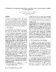
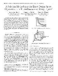
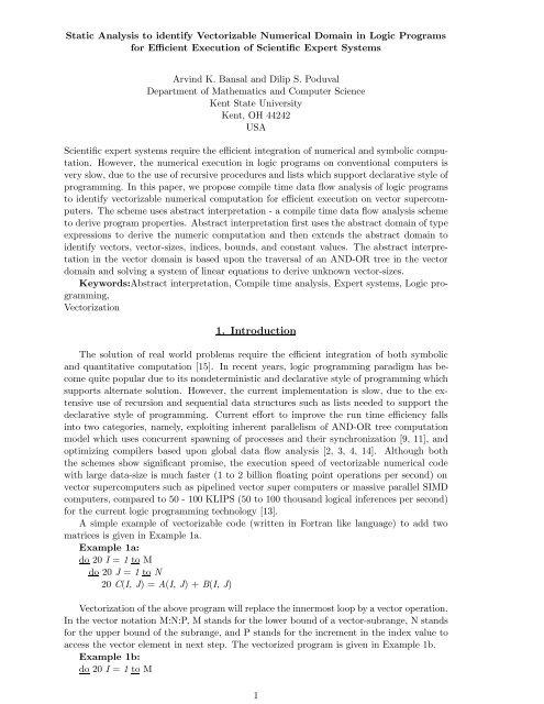
Static Analysis to identify Vectorizable Numerical Domain in Logic Programsfor Efficient Execution of Scientific Expert SystemsArvind K. Bansal and Dilip S. PoduvalDepartment of Mathematics and Computer ScienceKent State UniversityKent, OH 44242USAScientific expert systems require the efficient integration of numerical and symbolic computation.However, the numerical execution in logic programs on conventional computers isvery slow, due to the use of recursive procedures and lists which support declarative style ofprogramming. In this paper, we propose compile time data flow analysis of logic programsto identify vectorizable numerical computation for efficient execution on vector supercomputers.The scheme uses abstract interpretation - a compile time data flow analysis schemeto derive program properties. Abstract interpretation first uses the abstract domain of typeexpressions to derive the numeric computation and then extends the abstract domain toidentify vectors, vector-sizes, indices, bounds, and constant values. The abstract interpretationin the vector domain is based upon the traversal of an AND-OR tree in the vectordomain and solving a system of linear equations to derive unknown vector-sizes.Keywords:Abstract interpretation, Compile time analysis, Expert systems, Logic programming,Vectorization1. IntroductionThe solution of real world problems require the efficient integration of both symbolicand quantitative computation [15]. In recent years, logic programming paradigm has becomequite popular due to its nondeterministic and declarative style of programming whichsupports alternate solution. However, the current implementation is slow, due to the extensiveuse of recursion and sequential data structures such as lists needed to support thedeclarative style of programming. Current effort to improve the run time efficiency fallsinto two categories, namely, exploiting inherent parallelism of AND-OR tree computationmodel which uses concurrent spawning of processes and their synchronization [9, 11], andoptimizing compilers based upon global data flow analysis [2, 3, 4, 14]. Although boththe schemes show significant promise, the execution speed of vectorizable numerical codewith large data-size is much faster (1 to 2 billion floating point operations per second) onvector supercomputers such as pipelined vector super computers or massive parallel SIMDcomputers, compared to 50 - 100 KLIPS (50 to 100 thousand logical inferences per second)for the current logic programming technology [13].A simple example of vectorizable code (written in Fortran like language) to add twomatrices is given in Example 1a.Example 1a:do 20 I = 1 to Mdo 20 J = 1 to N20 C(I, J) =A(I, J) +B(I, J)Vectorization of the above program will replace the innermost loop by a vector operation.In the vector notation M:N:P, M stands for the lower bound of a vector-subrange, N standsfor the upper bound of the subrange, and P stands for the increment in the index value toaccess the vector element in next step. The vectorized program is given in Example 1b.Example 1b:do 20 I = 1 to M1

20 C(I,1:N:1) =A(I,1:N:1) +B(I, 1:N:1)Previous attempts to implement logic programming paradigm on vector supercomputers[6, 8] are not very successful for large programs due to(1) search for alternate solutions which require backtracking, (2)recursion and runtime creation of sequential data structures such as lists, (3) the bi-directional nature ofunification, and (4) the lack of vectorizable constructs such as Do -loop or For -loop inorder to retain declarative programming style.A practical scheme is to develop scientific expert systems (both symbolic and numericdomain) in logic programs to preserve the declarative style and rapid prototyping. Thesymbolic part is executed on conventional host computers whereas vectorizable numericalcode is automatically identified using compile time analysis and executed on vector supercomputers.The scheme will require:(1) compile time analysis to identify the vectorizable numerical code. This will requireidentification of definite iteration - iteration with predetermined number of iteration steps- related information and vector related information such as vector-size, the formulation ofindex-value to access vector elements etc.(2) data dependency analysis to identify sequentiality: suspension of a statement waitingfor the value(s) of a variable(s) in vectorizable code. In imperative languages, thereare three classes of dependences, namely, true dependence, anti-dependence, and outputdependence [17]. True dependence causes sequentiality by suspending the execution of astatement waiting for the value of an uninstantiated variable while anti-dependence andoutput-dependence cause sequentiality due to the reallocation of values to the same variable.Due to the absence of destructive nature of variables, logic programs exhibit only truedependence which is identified using compile-time producer-consumer relationship analysis[1, 2]. Producer-consumer analysis identifies those occurrences of the same variable variablewhich produce values and which consume the values.(3) translation of the vectorizable numerical domain to low level code on massive parallelsupercomputers. An intermediate step is to transform the vectorizable code to parallelizableFortran available on Cray supercomputers, or Parallel C available on massive parallel SIMDcomputers.A detailed schematic is given in Figure 1.This paper deals only with compile time data flow analysis scheme for the identificationof vectorizable numerical domain: identifying definite iteration, vectors, vector-sizes.Producer-consumer analysis has already been handled in detail [1, 2].The scheme is currently being implemented using Sicstus Prolog on Sun 3/60 system.The next section gives an overview of some unfamiliar terms and a compile-time analysisscheme to derive the numeric domain. Section 3 describes the characterizes the numericaldefinite iteration. Section 4 describes the compile-time analysis scheme to derive vector anddefinite-iteration related information. Section 5 concludes the work.2. BackgroundSome familiarity with logic programming is assumed [7, 10]. Briefly, a logic programis a finite set of Horn clauses of the form A :- B 1 , ..., B n (n ≥ 0). A computation of alogic program is a sequence of reductions (or resolution steps) from an initial query usingclauses from the program. At each stage the goal to be reduced must be determined bysome computation rule. A computation is successful if the empty goal is reached. In thiscase, the bindings of the variables in the initial query constitute a solution. A computationfails if there is no clause to reduce the chosen goal.In this section we briefly describe some less familiar terminology.Mode information is the set of instantiation state (represented in some abstract form)of the variables in a predicate before and after their execution.2

Figure 1: Integrating symbolic and numeric computing using static analysisAbstract Interpretation is a global data flow analysis technique to derive the propertiesof logic programs. It is based upon mapping the logic program into an abstract domain andtraversing an AND-OR tree in the abstract domain to derive the related properties. For theabstract domain of type expression, abstract interpretation derives the mode informationin terms of type expressions [1, 2, 3].In an indefinite iteration, a set of statements inside an iterative construct are executedindefinitely until the given condition is satisfied [12]. In a definite iteration, thenumberofiterations are finite and predetermined. A definite iteration has a lower bound, an upperbound, and an index which satisfy the loop invariant relationship lower bound ≤ index ≤upper bound. The index is not altered inside the set of statements and the bounds remaininvariant during the execution of an iterative loop [12].A vector is a sequence of elements in which each element can be accessed randomly andindividually using indexing. A homogeneous vector has all its elements bound to the sametype of object. From now onwards, we use “vector” to represent a numeric homogeneousvector unless otherwise stated. An input vector has all instantiated elements. An outputvector is uninstantiated before the execution of the predicate and instantiated during theexecution of the predicate. A vector-index is a variable whose value is used to access anelement of the vector.A tail recursive procedure has all the recursive clauses of the form p :- q 1 , ..., q n , p.The clause-head of the recursive clause has a recursive data structure with finite numberof elements which are consumed by the predicates q 1 , ..., q n and the procedure p is invokedrecursively for the rest of the elements.Prolog, the most popular implementation of logic programming paradigm, uses thepredicate functor(Structure, Name, N) to create a data structure of size N having nameName, and the predicate arg(Index, Structure, Element) to randomly access an elementElement in the structure Structure accessed by the index-value Index. Thisisequivalenttohandling single dimensional vectors. we define two similar predicates, namely, array(Array,Array-name, Dimension-list) andelement(Index-list, Array, Element) forthecreationofaN-dimensional array and accessing an element in the array respectively.3

Figure 2: Abstract InterpretationGiven two terms T 1 and T 2 , the subterms X in T 1 and Y in T 2 are called correspondingsubterms if they occur at the same position in T 1 and T 2 respectively.2.1. Abstract interpretation in type domainAbstract interpretation of logic programs is based upon the traversal of an AND-ORtree in type domain given a class of top level queries and a program.A type expression, defined recursively, is a type variable, a basic type, a functor witharguments as type expressions, a list of type expressions, a tuple of type expressions, and aset of type expressions. A basic type is described as an integer - denoted by Z, aconstantdenotedby C, an atomic type - denoted by A, a real type - denoted by R, oratypevariabledenoted by small Greek letters α, β, γ. Type expressions are denoted by τ. A set of typeexpressions is denoted by {τ 1 ,..., τ m }, where m ≥ 2. We denote a homogeneous list of atype expression τ by *: τ:< nesting-level >. For example, a list of integers is denoted by *:Z:1. A two dimensional matrix of real numbers is represented as a list of lists of reals anddenoted by *:R:2.There are four components of abstract interpretation, namely, Generalization, abstractunification, summarization, andconcretization [1,2,3,4](seeFigure2).Generalization maps logical terms onto the corresponding type expressions: variables aremapped to type variables and expressions are mapped to type expressions. Abstract unificationis analogous to unification and unifies two type expressions 1 . Summarization collects2 of mode information ( expressed as type expressions) derived from different clauses of aprocedure, and concretization associates the derived mode information with the correspondinglogical variables in the logic program. Given a program and a top level abstract query,abstract interpretation derives the binding of logical variables in terms of type expressionbefore and after the execution of the predicates. We illustrate the input and output of theabstract interpretation in Example 2. For further details, reader may refer to [1, 2].Example 2a:The example shows a simple program to add corresponding elements of two vectors Aand B and return the resultant values in an output vector C. The first and second argumentsrepresent input vectors A and B respectively, and the last argument represents the output1 process involves finding greatest lower bound of type expressions [1]2 process involves finding least upper bound of type expressions [1]4

vector C.add vector([X| Xs], [Y|Ys], [Z|Zs]) :- ZisX+Y, add vector(Xs, Ys, Zs).add vector([],[],[]).The intermediate code after the abstract interpretation is given in Example 2b. Eachobject is transformed to a triple { < data-object-name >, < input-mode >, < output-mode> }. For the query add vector(A, B, C), typical input modes for the variable A, B, C are*:R:1, *:R : 1, α respectively. The uninstantiation of the output vector C is indicated bythe type-variable α. After the abstract interpretation, the output modes for the variablesA, B, C are *:R:1, *:R:1, *:R:1 respectively.Example 2b:add vector([{ X, R, R}|{Xs, *:R:1, *:R:1 }], [{ Y, R, R}|{Ys, *:R:1, *:R:1}],[{ Z, α, R}| {Zs, β, *:R:1}]) :-{ Z, α, R}is { X, R, R} + { Y, R, R},add vector({ Xs, *:R:1, *:R:1}, { Ys, *:R:1, *:R:1}, { Zs, β, *:R:1} ),add vector({nil, nil, nil}, { nil, nil, nil}, {nil, nil, nil}).3. Characterizing vectorizable codeThe vectorizable domain is characterized by performing the same operation on a predeterminedsubrange of a vector(s). Since the number of iteration remains unaltered, definiteiteration is easily vectorizable.Consider the following example:Example 3a:do 20 I = 1 to 1020 C(I) =A(I) +B(2*I + 3)The corresponding vector code for the above program is C(1:10:1) = A(1:10:1) +B(5:23:2). Note that the value of the vector-index, used to access the elements in thevector B, increments periodically with a constant offset of 2 and an initial offset of 3.In logic programs, definite iteration is realized in two ways as follows:(1) Using tail recursive procedures which access the elements in the input or outputlists using a predetermined constant relative offset in each iteration step. The offset mayvary for different lists.(2) Using tail recursive procedures which access the elements of functors (or arrays)with variables acting as bounds and indices without explicit identification.Numerical procedures are identified by (1) using abstract interpretation in the typedomain to identify numerical subterm [1, 2], and (2) identifying the procedures which onlymanipulate numerical terms.3. 1 Handling numerical tail recursion with listsSince lists are used to represent any ordered sequence in logic programs, iterative operationon vectors are simulated using lists. However, the use of lists imposes two restrictions(1) the length of the vector is unknown, and (2) elements can not be accessed randomly.A list based version of the program Example 3a is given in Example 3b.Example 3b:add(A, [B1, B2, B3| Bs], C) :-add vector(A, Bs, C).add vector([A | As], [B1, B2 | Bs], [C | Cs]) :- CisA+ B1, add vector(As, Bs,Cs).add vector([],[],[]).In the above program, the initial offset (3 in Example 3a) to access elements of vectorB has been implicitly taken care of by explicitly representing first three elements of thesecond list in the clause-head of the top level procedure add/3. The constant offset invector-index to access elements in vector B has been implicitly taken care of by removingthe first two elements from the computation in the tail recursive goal of the recursive clauseadd vector/3.The vectorization of such code will need (1) identifying the size of the vectors (2)identifying the increment size and initial offsets of the vector-indices (3) formulation of5

number of iteration with respect to vector size and increment step, and (4) setting up andsolving a system of linear equations to derive the unknown range of the vectors involved inthe vector operation.3. 2 Tail recursion using functor/arraysSince functor or array allow indexing, the simulation of definite iteration uses index andbound without explicit identification. In iteration using functor/arrays,(1) the index is altered by a constant increment in each iteration step, (2) boundsremain invariant in the iterative loop. (3) The value of index is initialized to one of thebounds using unification during the call to the tail recursive procedure. The invariancelower-bound ≤ index ≤ upper-bound satisfied using an arithmetic comparison between theindex and bound in the recursive clause and equality test between the index and bound inthe base clause.A logic program version for the program in Figure 3a is given in Figure 3c.Example 3c:add(A, B, C) :-functor(A, ,N), functor(C, ,N), add vector((1, N), A, B, C).add vector((I, N), A, B, C) :-I < N, arg(I, A, X), I1 is 2*I + 3, arg(I1, B, Y), ZisX+Y, arg(I, C, Z), InextisI+1,add vector((Inext, N), A, B, C).add vector((N, N), A, B, C).In the above program, vector A, B, and C have been simulated using functors. The variablesI and N are used as the index and the upper bound respectively. Similarly, the values of thevariables I, I1, I are used to index the elements of the vectors A, B, andC. Vectorization ofsuch codes will need (1) identifying the index, the lower bound, and the upper bound, (2)identifying the variables used as vector-index to access elements in the individual vectors,(3) formulating and solving the number of iterations in terms of vector-range and theincrement step, and (4)setting up and solving a system of linear equations to derive theunknown vector-subranges which are being manipulated by the vector operation.3.3 Nested iteratationMultidimensional arrays are handled in logic programs using nested lists (or functors,or multidimensional array) and nested tail recursion. The nesting level is equivalent to thenumber of manipulated dimensions. Since index and bounds are the properties of a specificiterative loop, the classification of a subterm to index, bounds, or integer constants in onenesting level is independent of the classification of corresponding subterm in another nestinglevel. A subterm in an inner nesting level may act as a bound while the correspondingsubterm in an outer nesting level may act as an index. Similarly, a subterm in the an outerlevel may behave as a bound or integer constant while the corresponding subterm in aninner level may be an index.4. Extending abstract interpretation for vector analysisVector analysis primarily uses traversal of an AND-OR tree in the vector domain forthe refinement of the mode information derived from the type domain. Before the vectoranalysis, a static analysis identifies all the numerical tail recursive procedures [14].The input to vector analysis is a moded program derived from the abstract interpretationin the type domain, annotated identification of numerical tail recursive procedures, andvector-calling-mode of the query which includes both type and vector information. The outputof the analysis is a vector-moded program which contains vector and definite-iterationrelated information.Vector analysis has five components, namely, generalization, vector-unification, iterationanalysis,summarization, andconcretization as described in Figure 3.Generalization maps the mode information, derived from the abstract interpretationin type domain, to vector-domain. Vector-unification is analogous to unification of the6

Figure 3: Vector analysis of logic programsnumerical terms in the extended vector domain. Iteration-analysis is used in tail recursiveprocedures to identify the vector-size, the constant offsets for vector-indices, indices, andbounds. Summarization collects the refinement of the numerical terms in different clauses,subranges of the manipulated vectors, and the set of numerical values for the subtermsrepresenting numerical constants.4. 1 Vector domainWe extend the type domain to incorporate the information of bounds, indices, vectors,integer constants, and real constants. Integer is sub-classified to index - denoted by I, integerconstants - denoted by Z C , indexcons - denoted by I C , lower bound - denoted by B L , upperbound - denoted by B U , modified bound - denoted by B M ,andother-integers - denoted byZ φ . Indexcons I C represents those integers which are derived from an arithmetic operationof an integer of subtype a Z C on an integer of the subtype I or I C . The notion of I C isused to identify an index and definite iteration as described in Subsection 4.4. Similarly,we keep a type B M to keep track of the modification of possible bounds. An iterative loopcontaining a variable of the sub-classification B M can not be a definite-iteration.We also use variables in the vector domain to hold the values for integer constants,lower and upper bounds, length of the head part in a list, the offsets for indices, and thesize of vectors. We collectively refer to these variables as vector variables. We denote vectorvariables to hold the values of integer constants, lower bound of an iterative loop, or upperbound of an iterative loop by µ i , length of the head-part of a list in a clause-head by ηi H,length of the head-part of a list in a tail recursive subgoal by ηi B , lower bound of a vectordimension by δi U , upper bound in vector dimension by δL i , the lower and upper ends ofthe subrange of a vector by δi 1 and δi 2 respectively, constant offsets of vector-indices by ψ i ,nesting level in a list or number of dimensions in an array by κ i , the initial offset by ω i ,and the remaining elements in the lists in base clause of tail recursive procedure by ρ i .These notations have been used to set up and solve the system of equations as illustratedin Subsection 4.5.4. 2 Vector generalizationGeneralization takes the mode information, represented as a triple {predicate, callingmode,success-mode} from the output of abstract interpretation (as described in Example2b) and maps to the vector domain; a calling-mode in the type domain is mapped to thecorresponding vector-calling-mode and a success-mode in type domain is mapped to the7

corresponding vector-success-mode.In the vector-calling-mode (or vector-success-mode), an uninstantiated variable is representedby a type variable without any association, a single element is denoted as { , < basic-type >:1:< value> 3 , a N-dimensional homogeneous vector as { , #: < basic-type >: < number of dimensions >: lb 1 .. ub 1 , ..., lb N .. ub N: < value-list >}. 4 , a homogeneous list as { < type-variable >, *: < basic-type >: : < nested-value-list >}. Nested-value-list is used to pass the known values ofthe elements of declared finite lists. Other structures and non-homogeneous structures arerepresented as their representation in the type domain. Since user defined values do nothave any associated type variable they are represented by {$, < type >: < length >: }. For example, vector-generalization of a triple { a(4, X, Y), [(X, Z), (Y, α)],[(X, Z), (Y, *:R:1)]} will yield vector-calling-mode as a({$, Z C :1:4}, {α 1 , Z:1: µ 1 }, α 2 )and success mode as a({$, Z C :1:4}, {α 1 , Z:1:µ 1 }, {α 2 ,*:R: 1: µ 2 )}).4.3 Vector unification First the type-information in the vector-calling-mode(vectorsuccess-mode)of the calling goal is abstract unified with the vector-calling-mode(vectorsuccess-mode)of the clause in the type domain. Upon the successful abstract unification,the numerical terms in the vector-calling-mode(vector-success-mode) of the goal and vectorcalling-mode(vector-success-mode)of the clause are vector-unified in the vector domain to(1) pass the sub-classification Z C , I, B L ,andB U ,orI C in non-recursive procedures.Since these properties are specific to a particular nesting level of iteration, they can not becarried across nesting levels.(2) pass the value of Z C , B L , B U , and the constant part of I C .(3) match the values of the corresponding subterms which are of the subtype Z C .Sincethere may be a set of values associated with a subterm, vector unification finds the intersectionof two sets.(4) pass the dimensions of a vector.(5) vector-unify a homogeneous list with a vector to derive the value of the nestinglevel, number of elements in the list and number and size of dimensions in the vector. Theprocess involves coercing the nested list to a vector, equating the sizes of two vectors, andsolving the equations to derive the unknown values.(6) equate the values of two vector variables of two subterms associated with the sametype variable.For example, vector-term a({α 1 , Z:1:µ 1 }, {α 2 , Z:1:µ 2 }, {α 3 , Z C :1: 4}, [{α 4 , Z:1:µ 3 }|{α 5 ,*: Z: 1:µ 4 }]) vector-unifies with a({β 1 , I:1}, {β 2 , B U :1: 20}, {β 3 , Z C :1: 4}, {β 4 ,#:Z: 1: 1..20:µ 5 }) to give the common vector term as a(β 1 , I:1}, {β 2 , B U :1:20}, {β 3 , Z C :1:4}, { β 4 ,#:Z: 1: 1..20:µ 3 }) with vector binding as {µ 2 /20, δ1 1/ 2, δ2 1 /20, µ 5/µ 3 }. Notethat vector unification coerces the list to a vector which involves incorporating two vectorvariables δ1 1 and δ2 1 , equates the sizes of two vectors, and performs arithmetic operation todetermine the value of δ1 1 and δ2 1 .We omit a detailed algorithm due to space limitation.4.4 Identifying index/boundAt the beginning of vector analysis in tail recursive procedures using functor or arrays,the subterms in the tail recursive procedure representing an integer is undetermined andit could be any element in the set {I, B U , B L , Z φ }. An arithmetic operation on this setgives the set {I C , B M , Z φ }. The information from the vector-calling mode of the tailrecursive clause in the previous iteration step is kept and matched with vector-calling modeof the goal in the current iteration step. If any subterm satisfies the disambiguation rulegiven below, the subterm classification is given by the right hand side of the rule and otherpossibilities are pruned.3 Note that value can be a set of values since different clauses of a nondeterministic computation returndifferent values4 < value-list > is a linearized list of finite values and is used to pass the values of the individual elementsof declared finite vectors8

Disambiguation rules:match(II+ C 1, I I ) ⇒I. % identifying index ————– (1)match(B I+ 1 , B I ) ⇒B. % identifying bound or unaltered value —————– (2)At the end of the first pass, there must be at least one subterm which is identified asthe index. The absence of an index, indicates possible error due to indefinite loop or anindefinite iteration.After identifying the index, the second pass further derives/verifies the classificationusing the following rules.∧(value-of(Index) ≤ value-of(bound)) in recursive clause5∧(value-of(Index) ≥ value-of(bound) inbaseclause)value-of(constant offset in indexcons) > 0.———– (3)∧(value-of(Index) ≥ value-of(bound)) in recursive clause∧ (value-of(Index) ≤ value-of(bound) inbaseclause)value-of(constant offset in indexcons) < 0.———– (4)Both rules 3 and 4 are derived from the loop invariant relationship lower bound ≤index ≤ upper-bound. Rule 3 also identifies the bound as upper bound and rule 4 identifiesbound as lower bound. The value comparison relationship is either explicitly given by theprogrammer or it is implicit in the base case due to variable sharing. If two subterms whichare respectively identified as index and bound share the same type variable then they havethe same value.4. 5 Setting and solving system of linear equationsIn a tail recursive procedure, the values for the vector-size, constant offset, lower andupper bounds of the subranges of the manipulated vectors are not known. In order toderive this information, linear equations are set up and solved. Setting up of these equationrequires(1) identifying and comparing the length of the elements in the head part of the lists inthe head of the recursive clause and corresponding subterms in tail recursive goal to identifythe constant offset in vector-index.(2) setting an equation to derive number of iterations given the information about theknown vector size and the constant offset in the corresponding vector-index.(3) identifying those operation which equate a vector variable to a value or anothervector variable. These equations are derived in three ways:(i) explicit arithmetic operations involving vector variables. For example in example 3c,the statement I1 is 2*I + 3 relates the vector-indices I1 and index I.(ii) passing the values of vector variables as parameter values during vector unification.(iii) setting up equations to derive vector-size in terms of number of iterations and theconstant-offset in the corresponding vector-indices.Example 5:In Example 3b, following equations are set up and solved. We subscript the vectorvariableswith their vector names for identification. An equation which is applicable onall the three vectors is subscripted with i. Vector-variables have their usual meaning asdescribed in Subsection 4.1.(i∈{A, B, C })ηA H =1;ηH B =2;ηH C = 1; % identifying length of list-head in clause-heads;ηA B =0;ηB B =0;ηB 3 = 0; % identifying length of list-heads in clause-body;ω A =0,ω B =3;ω C = 0; % identifying initial offsetρ A =0;ρ B =0;ρ C = 0; % remainder elements in the clause-head of the base clauseψ i = ηiH - ηi B ; % finding increment step in index-valueδi 1 = δL i + ω i + ψ i - 1; % finding lower bound of the vector-rangeδi 2 = δ1 i + ψ i × (No. of iterations - 1) % finding upper bounds of the vector range.δi U = δi 2 + ρ i. % equating vector-size to upper bound of the vector subrange.Since there is only one level of nesting the number of dimensions in vector A, B, and C= 1. In order to find the number of iterations, one of the vector size has to be known which5 ∧ stands for ”and”9

is derived from the vector-analysis using value propagation of the integer constants.In example 3b, Given vector bounds δA 1 =1andδ2 A = 10, and the above equations, weget no-of-iteration = 10, ψ A =1,ψ B =2,ψ C =1,δB 1 =5,δ2 B = 23; δ1 C =1,δ2 C = 10.Using this vector information, we can derive the vector operation as C(1:10:1) = A(1:10:1)+ B(5:23:2).4.6 Vector summarizationSummarization collects the vector bindings derived from the various clauses of a nondeterministicprocedure. The process consists of(1) finding the union of the set of values of the subterms which occur at the sameposition and have subtype Z C .(2) collecting the specific values of the vector variables.(3) deriving the minimum of the lower bounds and maximum of the upper bounds returnedfrom different non-deterministic clauses. This is necessary because different nondeterministicclauses may invoke different iteration giving different size of the outputvectors.However, for the vector declaration, we have to use maximum size.4.7. Vector-analysis algorithmThe abstract query with the vector information is vector unified with the calling modeof the corresponding abstract clause 6 , and the bindings for the vector variables from vectorunification form the initial local environment E 0 for the clause. At any time, the vectorbindings for the next subgoal G i is derived by applying the bindings from last environmentstate E i−1 on the vector variables in G i . If the subgoal involves an arithmetic operationon vector variables then the new value of vector-variables is computed and stored in theenvironment. After the vector analysis of G i , the environment E i−1 is updated by composingthe vector bindings acquired from the success mode of G i to generate E i - a new version ofthe environment. For tail recursive procedures, a vector variable related equation which isexplicitly given by the user, is stored in the set of linear equations 7 . After encountering thetail recursive subgoal, the iteration analysis is performed to derive necessary informationabout vectors and iteration as described in Subsection 4.4 and 4.5. After deriving the successmode of all the vector-unifiable abstract clauses, the vector information is summarized. Thesummarized vector-mode is again vector-unified with the vector-success mode of the callinggoal to update the vector-information in vector-success mode of the calling goal. After thevector-analysis, concretization associates logical variables in the program to the derivedvector information.1 Conclusion and future workIn this paper, we proposed a practical view of integrating AI paradigm and scientific computationfor efficient execution of scientific computation without sacrificing the advantagesof declarative programming and rapid prototyping. We described a static data flow analysisscheme to identify definite iteration and vector information for effective vectorization ofnumerical domain on vector supercomputers. The scheme is based upon extending abstractinterpretation with abstract interpretation in type domain [1, 2]. The abstract domain hasbeen extended to include finer classification of numerical domain to include index, lowerbound, upper bound, integer and real constant, and other integers. The vector analysisis done in this extended domain and has five components, namely, generalization, vectorunification,summarization, iteration-analysis, and concretization. Iteration-analysis usessetting up of the equations to derive the size of the vectors and incremental steps to derivethe index value to find the next value in the vectors to be processed. Vector-analysis alsodisambiguates between index, bounds, and other integers.This paper does not describe the scheme to interchange the loops, fusion of two loops,or splitting of a loop into two loops to achieve maximum vectorization [17]. However, this6 vector-unification is attempted only if abstract-unification of goal-mode and clause-mode is successful7 equations are specific to a nesting level and stored in the specific set corresponding to the nesting level10

information is derivable once the information of the bounds and vector size has been derivedas shown in imperative languages by many researchers [17].References[1] Bansal, A. K., and Sterling, L. S., “A Scheme for Abstract Interpretation of Logic Programsusing Type Expression”, in Proc. of the International Conference on the Fifth GenerationComputer Systems, Tokyo, Japan, November 1988, pp. 422 - 429.[2] Bansal, A. K., and Sterling, L. S., “An Abstract Interpretation Scheme for Identifying InherentParallelism in Logic Programs”, in New Generation Computing, Volume 7, Number 2 & 3,January 1990, pp. 273 - 324.[3] Bruynooghe, M., and Jennsens, G., “An Instance of Abstract Interpretation Integrating Typeand Mode Inferencing”, Proceedings of the Fifth International Conference on Logic Programming,Seattle, USA, August 1988, pp. 669 - 683.[4] Debray, S. K., “Automatic Mode-inference for Prolog Programs”, Proceedings of the InternationalSymposium of Logic Programming, Salt Lake City, Utah, USA, 1986, pp. 78-88.[5] Fortran, X3J3/S8.104, American National Standard for Information Systems ProgrammingLanguage, June 1987.[6] Kanada, Y., and Sugaya, M., “A Vectorization Technique for Prolog without Explosion”, Proceedingsof the International Joint Conference of Artificial Intelligence, Detroit, Michigan,USA, 1989, pp. 151 - 156.[7] Kowalski, R., Logic for Problem Solving, Elsevier-North Holland, 1979.[8] Nilsson, M., and Tanaka, H., “A Flat GHC Implementation for Supercomputers”, Proceedingsof the Fifth International Conference of Logic Programming, Seattle, USA, August 1988.[9] Shapiro, E., Concurrent Prolog-Collected Papers, Volume I and II, MIT Press, Cambridge,Massachussets, 1987.[10] Sterling, L., and Shapiro, E., Y., The Art of Prolog, MIT Press (1986).[11] Takeuchi, A., and Furukawa, K., “Parallel Logic Programming Languages”, in Proceedings ofthe Third International Conference on Logic Programming, London, UK, pp. 242 - 254 (July1986).[12] Tennent,R.D.,Principles of Programming Languages, Prentice Hall, Newyork, 1982.[13] Warren, D. H. D., “An Abstract Prolog Instruction Set”, Technical Report 309, SRI International,USA, 1983.[14] Warren, D. H. D., “An Improved Prolog Implementation Which Optimizes Tail Recursion,Research Paper 156, Department of Artificial Intelligence, University of Edinburugh, Scotland,1980.[15] Wang, P. S., “FINGER: A Symbolic System for Automatic Generation of Numerical Programsin Finite Element Analysis”, Journal of Symbolic Computation, Volume 2, 1986, pp. 305 -316,Academic Press.[16] Weervarna, S., and Wang, P., S., “GENCRAY: A Portable Code Generator for Cray Fortran”,Proceedings ISSAC’89, the 1989 International Symposium on Symbolic and AlgebraicComputation, Portland, Oregon, July 1989, pp. 186 - 191.[17] Wolfe, M., Optimizing Supercompilers for Supercomputers, MIT Press, 1989, 176 pages11