Pr obability Distributions

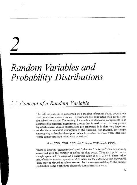
Random Variables and
Pr obability Distributions
J."/ Concept af a Random Variable
The field of statistids is concerned with making inferences about populations
and pop-ulation- qhar.actffistics. Experiments are'ioiiducied with results that
'are
subject to chance. The testing of a number of electronic components is an
example of a statistical experiment, a term that is used to describe any process
by which several chance observations are generated. It is often very important
*) tg allocata".a nuqerical description !9 the outcome. For example, the sample
space giving a detailed description of each possible outcome when three elect1o-9jc_.qppponents
are tested may be written
5: {NNN, NND, NDN, DNN, NDD, DND' DDN,,DDD\, '
- . I,r
where N denotes "nondefective" and D denotes "defecti#.n'One is naturally
concerned with the number of defectives that occur. Thus each point in the
sample space will be assigned a numericsl value of 0, I, 2, or 3. These values
are, of course, random quantities determined by the outcome of iei*priiilinf.
fn*y *"y be viewed as values assumed by the random uariable' X, the number
gi-Ce,{ectivg items when three electronic components are tested.
4 j

44
Definition 2.1
Example 2.1
,n/ 't..t
- t,).,a'v i *^
\*j .,:.r :,-!,..r .J1.1
Example 2.2
Ch. 2 ' Rsndom Variables and Probability Distributions
.4 random variable a func tion tAq- qs ssCt:q! e,s q-r gql luy1b-91-Vtt!-e rch:JSmep in
the.s*mple space.
We shall use a capital letter, say X, to denote a random variable and its
corresponding small letter, x in this case, for one of its values. In the electronic
component testing illustration above, we notice that the random variable X
assumes the value 2 for all elements in the subset
5: {DDN, DND, NDD}
of the sample space S. That is, each possible value of X_represents an eveg-t
that is a subset of the sample space for the given experiment.
Two balls are drawn in succession without replacement from an urn containing
4 red balls and 3 black balls. Th_e pA-s-lible outcomes and the valueg-;r of
the random variable
", *$j:I it ll1".::ryEt-q!9{ b{ls' are
Lol"", t*r*qh
Sample Space v"
RR
RB
BR
BB
A stockroom clerk returns three safety helmets at random to three steel mill
employees, who had previously checked them. If Smith, Jones, and Brown, in
thai oider, receive one of the three hats, list the sample points for the possible
orders of returning the helmets and find the values m 9'-f lhe random variable
M that represents the number of lneclSatches'
Salution. If S, J, and B stancl for Smith's, Jones', and Brown's helmets, respectively,
then the possible arrangements in which the helmets may be returned
and the number of correct matches are
2
1
1
0
Sample Space fl
SJB
SBJ
JSB
JBS
BSJ
BJS
3
1
1
0
0
1

iec. 2.1 ' Concept of a Rantlom Vaiable
In each of the two preceding examples the sample space containp a finite
number of elements. On tne other hand,-yhg! a d-i9 i1lhJown unti! a 5 occurs,
..*a'afmna-sempii slace m-rmannnena_ing sequence of elements,
s: {F, NF, NNF, NNNF,...},
where F and N represent, respectively, the occurrence and nonoccurrence Of a
5. But even in this experiment, the number of elements can be equated to the
number of whole numbers so that tllere is a first element, a second element, a
ihird "taro"nt, and so on, and in this sense can be counted'
tleffnitiOn 2.2 If a sample space contoins a fnite number of possibilities or an unending sequence
with as m-any elements as there are whole numbers, it is called a discrete sample
space.
Theoutcomesofsonrestatisticalexperimentsmaybeneitherfinitenor
countable. Such is the case, for example,-when one conducts an investigation
measuring the distances that a certain -aiii oi automobile will travel over a
test course on 5 liters of gasoline. Assuming distance to be a vari-
Of*;i;i
able measured to any degree of accuracy, then clearly we have an infinite
number of possible distanies in the sample space that cannot be equated to
the num-beF-o$*whsle*numher$, Also, if one were to record the length of time
i;;;il;cal reaction to take place, once again the possible time intervals
making up our sample ,puc" utt infinite in number and uncountable' We see
now that all sample spaces need not be discrete'
illdrution 2.3 If a sample space contains on infnite numbey of possibilities equal to the number of
pointson.alinesegment,itiscalledacontinuoussamplespace.
@
A random variable is called a discrete ranilom variable if its set of possible
outcomes is countable. Since the possible values of Y in Example 2'1 are 0, 1,
uii z, and the possible values of M in Example 2.2 are 0, 1, and 3, it follows
that y and M are discrete random variables. When a random variable can
take on values on a-c-qn-tiDuqEs- scgle, it is called a continuous random vsriable'
oil"o ttr" possible nutu"r of i continuous random variable are precisely the
same values that are contained in the continuous sample space._ Such is the
case when the random variable represents the measured distance that a certain
*utd oiuotomobile will travel over a test course on 5 liters of gasoline'
.^.. 2 | i; most practical problems, 99!-4_Luo-qs- random- YaqAllgS -Lep!9!9-nt-"msa-
--'zF
I
*r,"--- -*,' k / w-94-ngj9,cua3se!!9uoUt"-frtigltlt*trehtt, telqpqrallules, distaqce$, or life
ffi:- ,--t'' ,frf I ffi-' wt*"* airdt" ."tta"- such as lhe
""ri"ut"-*reBL?,seatJpunL-da-ta,
{, ;ffi; sf dged="_"t a_sample of k itp$s qltlhe luslbpr of highway-,iel.a-lities
drn ",*' *
v
14-
-
rdi - f-ryrt;-iry4-gvel 59i*1har-the.-rand-om
-stata
:tr*
;;;U"t of corrgct hat rnatches' ,
45
variables Y an{.M of E11m--
pd;.i;;a fi-ioth repreienicount data, f the number of red balls and r14

46
'r"*, @
t jr' ++r
,r' !' I J '
6. pt( '1t
lTr
t_plf H
Ll T KY ,?- 1 rrl-l
"'. I'li"li.{ r. TT Ff
"4
Ch. 2 ' Random Variables and probability Distributions
2.2 Discrete Probability Distributions
i t\ ! .r i
-.ir')' i't/:{i
!1ri":!r. :r,ii
t:
..,:.t . ,.-.,.i.. i
i:
,\ -'s 1 ,'
,{ dis.c-r91e randgm variable ?s-suTes each of its values with a cer1ain-probabil"-
, ity"Jn the case of tossing a coiiTfi-ree-iiffi&;'tr6-14;it6l" x,-iepresenting the
number of heads, assumes the value 2 with probability 3/g, since 3 of the g
equally likely sample points result in two heads and one tail. If one assumes
equal weights for the simple events in Example 2.2, the probability that no
employee gets back his right helmet, that is, the probability that M assumes
the value zero, is l/3. The possible values m of u and theii probabilities are
given by
P(M : m) 111
326
L-l
le(tL
Note that the values of m exhaust all possible cases and hence the probabilities
add to l.
Frequently, it is convenient to represent all the probabilities of a random
variable X by a formula. such a formula would necessarily be a function of the
numerical values x that we shall denote by f (x),g(x), r(x), and so forth. Therefore,
we write /(x) : P(X : x); that is, /(3) : p(X: 3). The set of ordered
pairs (x,/(x)) is called the probability function or probability distribution of rhe
discrete random variable X.
Definition 2.4 The set of ordered pairs (x,f (x));s a p1qlghiljlx.fg4plior-r, probability mass funcrion,
or ppla-bllly ,Qqt1ilrrlion of the discrete random uaiiable X rf,for each possible
outcome x'
lr'r
t>' o
l./(x)>0. 2it"':"t {"
2.lf1x1: t.
Z. PtX:;r) :/(x).
Example 23 A shipment of 8 similar microcomputers to a retail outlet contains 3 that are
defective. If a school makes a random purchase of 2 of these computers, find
the probability distribution for the number of defectives.
sslntion. Let X be a random variable whose values x are the possible
numbers of defective computers purchasec by the school. Then x can be any of

Sec. 2.2 Discrete Probability Distributions
. /:\
" r;10 ,0
' - t /to1:P(X:0):7f:X'
the numbers 0, 1, and 2. Now'
: t."
. '.: ... :,."
e\ ty'
j - ,4ri*rl.:,*{
. -1
.]'
'*l
" i i. ,.
:- ': !''|,r"r /i t li { ' (
f (2) : P{X :2) :
'ii", ;il;."i"uii',v Ji',ribuiion ol X is
Example2.4If50%oftheautomobilessoldbyanagencyforacertainforeigncarare
equrppedwitlldiesele4g!ne$n.a"r"'-"r"foitheprobabilitydistributionof
_ r, tt. n,i,.,'U", dl ales66"olJilnons "'^'"-' -\:..--
' j
---
''/
\,1
0
the next 4 cars sold bv this agency'
,.*. 'i- ^Solulion,$iace..the probability of selling a diesel model or a gasoline model is
0.5, ;;;';i: tO'Uoints in the sample space are equally iikely to occur' There-
,or","iil"'o*;t'";;;; ;11 prouuuititi"t, and.also for our function' will be
i6..fg-qbt-aa$9-lu-loberofw'ays.ofselling3diesel..models"weneedtocon.
*

48
Ch. 2 ' Random Variables and Probability Distributions
Definition2.5,,'oW)ofadiscreterandomuariableXwithprobabiIity
f iu 1-
* il} '''
fL?;:'
-iti= /"
, i,,)= 'lr
r'(x): P(X

l
Discr ete Pr obabilit y Distributions
6l t6
s lt6
4l16
3l t6
2lt6
Figure 2.1 Bar chart.
I lt6
It is often helpful to look at a probability distribution in graphic form. one
might plot the points (x,,f(x)) of Example 2.4 to obtain Figure 2.l.By joining
the points to the x axis either with a dashed or solid line, we obtain what is
commonly called a bar chgrt. Figure 2.1 makes it very easy to see what values
of X are most likely to occur, and it also indicates a perfectly symmetric situation
in this case.
Instead of plotting the points (x,"f(x)), we more frequently construct rectangles,
as in Figure 2.2.Herc the rectangles are bonstructed so that their bases of
equal width are centered at each valus x and their heights are equal to the
corresponding probabilities given by"f(t).The bases are constructed so as to
leave no space between the rectangles. Figure 2.2 is called a probability histogram.
I
since each base in Figure 2.2 has'.nit width, the P(x : x) is equal to the
area of the rectangle centered at x. Even if the bases were not of unit width' we
could adjust the heights of the rectangles to give areas that would still equal
the probabilities of X assuming any of its values x. This concept of using areas
to represent probabilities is necessary for our consideration of the probability
distribution of a continuous random variable'
The graph of the cumulative distribution of Example 2.5, which appears as a
step function in Figure 2.3, is obtained by plotting the points (x, F(x))'
6l 16
s lt6
4lt6
3116
z.l t6
I lr6
0l
Flgure 2.2 Frobability histogram.
49

50 Ch. 2 ' Random Variables and Probability Distributions
I
314
t12
t14
I
?------------J
I
Figure 2.3 Discrete cumulative distribution.
I
r-r___________l
I
r------J
I
Certain probability distributions are applicable to more than one physical
situation. The probability distribution of Example 2.4, for example, also
applies to the random variable Y, where Y is the number of heads when a coin
is tossed 4 times, or to the random variable W, where W is the number of red
cards that occur when 4 cards are drawn at random from a deck in succession
with each card replaced and the deck shuflled before the next drawing. Special
discrete distributions that can be applied to many different experimental situations
will be considered in Chapter 4.
2.3 Continuous Probability Distributions
>1
'.(' ,J (.\, A continuous random variable has a probability of zero of assuming exactlv
.._ - .',,,,:--'-':-- .-
- ----=-
m €-it-61-m-vamECTonsequentlylitFprobability distribution cannot be-givet. in
--
-''''t -=:---
,l -..:^' ,'ti\.! q ffid, ibfrlnt first this may seem startling, but it becomes more plausible
.\ L .'; -f' E r- .r
.... 1i {i.. -, r,, ! - when we consider a particular example. Let us discuss a random variable
.*t.o ,,u }f,.. .ll, whose values are the heights of all people over 2l years of age. Between any
-" \" {.
t
lr. . two values, say 163.5 and 164.5 centimeters, or even 163.99 and 164.01 centit
, \^.',' meters- there are an infinite number of heishts. one of which is 164 centimeters.
i' -ndL+r" - q The prdba-.fiIi1! of selecting a person at random w-ho is qx4ctly 164 centim_eters
, A '' ., / tall and not one of the infinitely large set of heights so close to 16a centimeieii
^
, s-"Fr*
"ntr''
,nN, ] that you cannot humanly measure the difference ltg:fr,ole, and thus we assign
M p I"-t [a probability of zero to the event. This is not the case, however, if we,f-alk
@ \t ,^5 I-1;d'
W \u .,id}" not more than 165 centimeters tall. Now we are dealing with an '$''
interval rather
about the probability of selecting a person who is at least 163 centimeters'6u1-
tttun u poini uutu" of our *nao* variable.
We shall concern ourselves with computing probabilities for various intervals
of continuous random variables such as P(a < X < b), P(W > c), and so
forth. Note that when X is continuous
P(a < X < b) : P{a < X < b) + P(X : b
: P(s< X

Scc. 2-3
I
C ontinuous Pr ob abilit y Distributions
(c)
Figure 2.4 Typical density functions.
9 ), .That is.. it does not matter whether we include an end point of the interval or
e | - not. This is not true. though. when X is discrete.
Although the probability distribution of a continuous random variable
cannot be presented in tabular form, it can have a formula. Such a formula
would necessarily be a function of the numerical values of the continuous
- vaiiable X and as such will be represented by the functional notation/(x). In
, ^,\. / dealing with continuous variables,/(x) is usually called the probability density
[* function, or simply the density function of X. Since X is defined over a continuous
sample space, -.:,',t5 it is possible for/(x) to have a finite number of discontin-
.;.. f uities. However, most density functions that have practical applications in the
.. ,, analysis of statistical data are continuous and their graphs may take any of
' ,, , several forms, some of which are shown in Figure 2.4. Because areas will be
.' ,-, used to represent probabilities and probabilities are positive numerical values,
the density _fu,Irgli_on must lie entirely above the x axis.
A probabilitv itv densitv density function lunction is constructed so that the area under its curve
bounded bv the x axi ualtolw qyer,ltlqlg-lgr el X_!gI
x) is defined. Should this range of X be a finite interval, it is always
possible to exten interval to include the entire set of real numbers by
defining/(x) to be zero at all points in the extended portions of the interval. In
Figure 2.5, the probability that X assumes a value between a and b is equal to
the shaded area under the density function between the ordinatss at x : o and
x : b, and from integral calculus is given by
tl, 1
I P@. x

52 Ch. 2 ' Random Yariables and probability Distributions
Figure25 P(a

I
Sec. 2.3 . Continuoas Probability Distributians
Definition 2.7 The cumulative rlistribution F(x) of a continuous ranilom Dariable X with density
function[(x\ k giaen by
for-m

Exercises
Ch. 2 ' Random Variables and probability Distibutions
The cumulative distribution F(x) is expressed graphically in Figure 2.6. Now,
P(0 < X < 1) : r(1I_ F(0) : 4 _ t : *,
which agrees with the result obtained by using the density function in Example
2.6.
" l. Classify the following random variables as discrete 06.
or continuous-
the number of automobile accidents per year
in Virginia.
Y: the length of time to play 18 holes of golf.
M: the amount of milk produced yearly by a-./7.
particular cow.
N: the number of eggs laid each month by a
hen.
P: the number of building permits issued each
month in a certain city.
Q: the weight of grain produced per acre. '/8'
,2. An overseas shipment of 5 foreign automobiles
contains 2 that have slight paint blemishes. If an
agency receives 3 of these automobiles at random,
list the elements of the sample space S using the '/9.
letters B and N for ..blemished - and
" nonblemished," respectively; then to each sample
point assign a vdlue x of the random variable X
representing the number of automobiles purchased
by the agency with paint blemishes. ./10t
3. Let W be a random variable giving the number of
heads minus the number of tails in three tosses of
a coin. List the elements of the sample space S for /ll.
the three tosses of the coin and to each sample --'
point assign a value w ofW.
/4. A cain is flipped until 3 heads in succession occur.
List only those elements of the sample space that
require 6 or less tosses. Is this a discrete sample
space? Explain.
v'5. Determine the value c so that each of the follow- lL
ing functions can serve as a probability distribu-
tion of the discrete random variable X:
t(a) f(x) : c(x2 + 4) for x : 0, 1,2,3;
(b) f(xt: "(:)(,I.) for x:0, r,2
13'
From a box containing 4 dimes and 2 nickels, 3
coins are selected at random without replacement.
Find the probability distribution for the total T of
the 3 coins. Express the probability distribution
graphically as a probability histogram.
From a box containing 4 black balls and 2 green
balls, 3 balls are drawn in succession, each ball
being replaced in the box before the next draw is
made. Find the probability distribution for the
number of green balls.
Find the probability distribution of the random
variable 17 in Exercise 3, assuming that the coin is
biased so that a head is twice as likely to occur as
a tail.
Find the probability distribution for the number
of jarz records when 4 records are selected at
random from a collection consisting of 5 jezz
records, 2 classical records, and 3 polka records.
Express your results by means of a formula.
Find a formula for the probability distribution of
the random variable X representing the outcome
when a single die is rolled once.
A shipment of 7 television sets contains 2 defective
sets. A hotel makes a random purchase of 3 of the
sets. If X is the number o[ defective sets purchased
by the hotel, find the probability distribution of X.
Express the results graphically as a probability
histogram.
Three cards are drawn in succession from a deck
without replacement. Find the probability distribution
for the number of spades.
Find the cumulative distribution ol the random
variable l/ in Exercise 8. Using F(w), find
(a) P(W > o);
(b) P(-t

;ec. 2.5 Joint Probability Distibutions
decimal point, each repeated five times such
that the double-digit leaves 00 through 19 are
associated with stems coded by the letter a;
leaves 20 through 39 are associated with stems
1.5 Joint Probability Distributigr'!
63
coded by the letter b; and so forth' Thus a
number such as 1.29 has a stem value of lb and
a leaf equal to 29'
(b) Set up i relative frequency distribution'
(e)ourstudyofrandomvariablesandtheirprobabilitydistributionsinthepre.
ced i n g sec ti o ns * ;';.;;;;t'd tggl,':q iT'l'i " " il' l++"-:p:"="-:: i: :l:: H
f*.";0 ".
;I;i,"li3:.!
we w€ might trrrBrrl measure rrrv4Jurv the r'v 'ving -:-^ .^ ^ +rr,^
rise to a two-dimensional .ri-ancinnal
from a controlled chemical experiment gr
sample space consistd^;ilil;;tcomes (p' :l' "-t "t"::lT be-interested in
the hardness H and ,"i'if" T of cold-drawn copper resulting in the
'tt""gth
ourcomes (h, 4. In ;;; io J"i".-ine the likelihood of success in college'
"
based on high school J*", on" might use a three-dimensional sample space
andrecordforeachindividualhisorheraptitudetestscore,highschoolrank
in class, and grade-poi;; ;;;;;g" at the endof the freshman year in college'
If X and y ur" t*o-dlr"."tJ."rroom variables, the probability distribution
lor their simultaneous occurrence can be represented by a function with values
puit or I;;;;";;"v
*ru"t 1t' v) within the range of the random variables X
and y, It is customary ,o-i"r"t ,. this function as the ioint probability distribution
of X and Y' Hence, in the discrete case'
f{x,Y}:P(x:x'Y:Y);
that is, the values /(x, y) give the probability that outcomes x and y occur at
the same time' For if aielevision set is to be serviced and X rep-
"*L'u:ptin,
resents the age to ttre iea're'i y"u' of the set and Y represents the number of
defective tubes in trr" r"t, it"n i6,z)is the probability that the television set is
5 years old and needs 3 new tubes'
2"8 The function f (x, y)is a ioint probability distribution or probability mass function o/
the discrete 'lon''lo^ uariables X and Y if
7. f (x, y) > 0 for all (x, Y)'
, \\.f(x, y): 1.
3. P(X:x,Y:Y):f(x,Y)'
For any region A in the xy plane' Pl(X' Y) e Af : I I 16' il'

64 Ch. 2 - Random Yariables and Probability Distributions
Example 2.8
i.,. j
Two refills for a ballpoint pen are selected at random from a box that contains
3 blue refills, 2 red refills, and 3 green refills. If X is the numbcr of blue refills
and Y is the number of red refills selected, find (a) the joint probability func-
{oni(x, d, ana 0)"1(X,Yf e Af,whdre.4 is the region {(t, y)lx + y < 1}.
Solation
(a) The possible pairs of values (x, y) are (0, 0), (0, 1), (1, 0), (1, 1), (0, 2), and
(2,0). Now,/(0, 1), for example, represents the probability that a red and a
green refill are selected. The total number of equally likely ways of selec-
ting any 2 refills from the t - 0 : 28. The number of ways of selecting I
red from 3 red refills and I green from 3 green refills is (?Xi) : 6. Hence
,f(0, 1) :6128 -- 3114. Similar calculations yield the probabilities for the
other cases, which are presented in Table 2.6. Note that the probabilities
sum to 1. In Chapter 3 it will become clear that the joint probability distribution
of Table 2.6 can be represented by the formula , !
' -o;
for x : A, \2; | : 0, 1,2;0 < x + Y < 2.
(b) P[(X, Y] e A]: P(X + Y < 1)
:"f(0, 0) +/(0' 1) +/(l' 0)
:rr3+*+*
:&
., \-00(,-1-,)
Jtx,y):T__,,
\r/
Table 2.6 Joint Probability
Distribution for Example 2.8
f(x, v)
0
yl 2
Column
Totals
x
o ii i^.\ 2
'_tle
l28l28i
i -r- I -r-
,1411+
rli
i 2R:i
-r ,r-r i
-L
28
La. 2g 2a
i
l-.r'
t,
Row
Totals
ll'
2A
3
7
-L
2A
I

I
Sec. 2.5 Joint Pr ob abiltt y Distributions
65
When X and Y are continuous random variables, the joint density function
f(x,y) is a@, and P[(X, Y\ e Af, where,4 is any
region in the xy olane- is eoual to tht uolg-e of th" !!ght t
the base .4 and the surfiG]-
Definition 2.9 ,**;1t?;f(*,y\ isc jointdensityfunction of thecontinuousrsndomoariablesX
l.f(x,v)>
O for all (x, y).
fa fo
r. f(x, y) dx dy : 1.
.J__ .l__
3. Pt(x, Y) e Af: iitO, fl dx dy
for any region A in the xy plane.
Erample Z.g ) A candy company distributes boxes of chocolates with a mixture of creams,
' toffees, and nuts coated in both light and dark chocolate. For a randomly
selected box, let X and Y, respectively, be the proportions of the light and
dark chocolates that are creams and suppose that the joint density function is
given by
(a)
(b)
f(x, v): {::t
Verify condition 2 of Definition 2.9. *)
Find P[(X, Y) e A], where.4 is the region
+3y), 0

66 Ch. 2 ' Random Variebles anil Probability Distributians
(b) P[(x, Y) e Af
:P(o

t
J oint ProbsbilitY Distributions
Lxample 2.11
2
P(X:1):9(1):lf0,t)
v=0
:/(1,0) +/(1, 1) +f(r,2)
--&+rnr+o:4;'
2
a P(X : 2) : g(2) : L f(2, v) :f(2,0) + f(2' r) + f(2'2)
)=0
:*+0+0:*,
which are just the column totals of Table 2'6' In a similar manner we could
show that the values "i-lttyl "* given by ll9 to't" totals' In tabular fornr' these
margittut distributions may be written as follows:
Find g(x) and h(y) for the joint density function of Example 2'9'
Solution. BY definition'
ra f r')
s$): v)
.J__r,*, dY : (" + 3Y) dY
.|. ;
4xv 6v'lt= 1 4x * 3
: s *lol,=o 5
for 0 < x ( 1, and g(x) : 0 elsewhere' Similarly'
ro lr )
h(y): .|_to, r) dx: J. i,t.
-4r t_3v\
)
for 0 < Y S 1, and h(Y) :0 elsewhere'
+ 3) dx
The fact that the marginal distributions g(x) and hlyYt: inlef the prob*
abitity distributions ,iiir-iiai"idual variiL. X "nA Y alone can easily be
verified by showing ;1";;;""ditions of Definition 2.4 or Definition 2'6 are
..iitn"a. io, examplc, in the continuous case
[* n(r) ar: l* i' ,,', v\ dv dx: I
j-- J-o J-o
lu:
67

68 Ch. 2 ' Random Yariables anil Probabtlity Distributions
and
P(a < X < b) : P(a < X 1b, -co < Y < co)
lb l*
:l I f@,v)dvdx
JoJfb
: I g$\ dx'
Jo
In Section 2.1 we stated that the value x of the random variable X represents
an event that is a subset of the sample space. If we use the definition of
conditional probability as given in Chapter 1,
P(Bl A) :
P(A o B)
P(A)
P(.4) > 0,
where / and B are now the events defined by X : x and Y: y, respectively,
then
P(Y : ylX: x): P(X--x,Y:l)
P(X : x\
: IJ+!, s(x) > o,
s@)
when *Itlr X and Y are disglgte'raadam-raua-bles*."
""i Aiffilt t; show that the function f(x,y\ls!), which is strictly a
function of y with x fixed, satisfies all the conditions of a probability distribution.
This is also true when/(x, y) and g(x) arc the joint density and marginal
distribution of continuous random variables. Expressing such a probability
distribution by the symbol/(y lx), we have the following definition.
Definition 2.11 Let X and Y be two random variables, discrete or continuous. Ihe*cgndjtional
distribution of the random uariable Y, giun thot X : ,, it gir.4
f ulx) : W, s(x) > o.
-<
Shnilarly, the conditional distribution of the random variable X, giuen that
Y : y, is giuen by
f(xli:W, h(v)>0.
If one wished to find the probability that the discrete random variable X
y, wE
falls between a and b when it is known that the discrete variable f -
evaluate
P(a < X < blY : y) : I.f(rly),

J oint Pt obabilitY Distributions
where the summation extends over all values of X between a and b' When X
and Y are continuous, we evaluate
lb
P(a < x < blY : !) : J"ft*li a*'
Solurton.
Now
Therefore,
w" needl find/(xly), where y : 1' First we find that
h(l) = i .f(x, 1): * + * +o :+'
x=O
f(x, l) t .(r, ,), x : o, l, Z.
/(xl1):7f=3r
/(0t1) : +f(a,l):
(3x*): *
/(11 1) : !f(r,l) : (3x*) : I
/(21 1) : zf {2,1) : (3x0) : 0
and the conditional distribution of X' given that Y : l' is
f(x I l)
FinallY, O r€t Y: 1):.r(ol1): *'
bnra
G)Therefore, if it is known that 1 of-the 2 pen refills selected is red' we have a
-;;;;;;uiiv
"qutt to-r/z tt'ut the other refill is not blue'
/-' ^ r-^^+r^n Y nf male runners and the fraction Y of female
*fu "qlp1s-z,reJw.*Jn'ff JfiT'*,f,*?:::,':#TFilil#;ii":"*'densitv
function
o!\(t{r
r(x, y): til' I,i"J,i;.
o < / < 1
Find g(x), h(v),/(y I x)' and determine the probability that f:Y-": '1"'n
69
1/8 of the
women entered i' u pJrti"oru, marathon d;lly i"tshed if it is known that
;xafi; ip;i;" male runners completed the race'

70 Ch. 2 . Random variables snd probability Dis*ibutions
Example 2.14
Solution.
and
Now,
By definition,
fo lx
s@): I f6, y) dy : | 8xy dy
J-- Jo
lY=t
:4xy2l :4xt, o

J oint Probability Distributions 7I
Therefore,
and
:n"ru mi,stic al Independence
f (xlt):
t
(t
Pl -
\4
f (x, y) _ x(l + 3y2)14
h(y) - (1 +3y\2 -/". -tl
< x

7 2 Ch. 2 - RandoTn Variables and Probability Distributions
The continuous random variables of Example 2.L4 are statistically independent,
since the product of the two marginal distributions gives the joint density
function. This is obviously not the case, however, for the continuous variables
of Example 2.13. Checking for statistical independence of discrete random
variables requires a more thorough investigation, since it is possible to have
the product of the marginal distributions equal to the joint probability distribution
for some but not all combinations of (x, y). If you can find any point
(x, y) for which/(x, y) is defined such that/(x, y) + S6)h(y), the discrete variables
X and Y are not statistically independent.
Example 2.15 Show that the random variables of Example 2.8 are not statistically independent.
Solution.'Let us consider the point (0, 1). From Table 2.6 we find the three
probabilities,f(0, 1), g(0), and i(1) to be
Clearly,
/(0' l): t )
s(o): I f$, v): * +
'=O
2
h(1): I ,f(x, 1): * +
x=O
/(0, l) # g9)h(t),
3 r I
14r 28-t4 -l-
*i + o:;.
and therefore X and Y are not statistically independent-
All the preceding definitions concerning two random variables can be generalized
to the case of n random variables. Let f(xr, x2, ..., x,) be the joint
probability function of the random variables Xy Xr, ..., X,. The marginal
distribution of Xr, for example' is given by
s(x):I I f(xyxz,...,xJ
for the discrete case and by
s(xr): I: f
* .rtrr, xz, ..., xi;,) dx, dx3 '' ' dxn
for the continuous case. We can now obtain ioint marginal distributions such
as @(x1, xr), where
It L f@r,
xn
l-t
6(xt, xr) :
xz, -.', Xo)
ll- "J-'-tt'"x2r"'r
(discrete case)
x^) dx3 dxa "' dx, (continuous case).

t
Sec, 2.5 Joint Probability Distributions
one could consider numerous conditional distributions. For example, the joint
conditional distribution of Xr, X.r, and X., given that Xnl rn, X, : x5, ...,
X n : x,, is written
f (xt, xz, xtlx+, xs, ..., xn) : f lxt xz' ' ", x)
"' g(x+, x5, .. ., xJ'
where g(xa, xs,..., x,) is the joint marginal distribution of the random variables
Xn, X s, ..., X n.
A generalization of Definition 2.12 leads to the following definition for the
mutually statistical independence of the variables X ,, X r, . .-. , Xn.
mk'finition 2.13 Let Xr,Xr,.", xnbenrandomuariobles,discrete or continuous,withjointprobability
distribution f (x,., xr, . . ., xo) and marginal distributions fr1xr1,, yrlxrj, ...,
f,(x,), respectiuely. The random uariqbles X ,, X r, ..., Xn or, ,iti'ti b:i*iiually
statistically independent if and only if
for all (xr, x,..., Xn) within their range.
f (x,., xr, .. ., x,) : fr$)fz(xz) . . . f ,(x,)
frample 2.16 Suppose that the shelf life, in years, of a certain perishable food product packaged
in cardboard containers is a random variable whose proUaUitity density
function is given by
tvt:{'^"
[0,
x>o
elsewhere.
Let X r, Xr, and X, represent the shelf lives for three of these containers
selected independently and find p(X, < 2, 1 < X, 1 3, X, > 2).
Solution. Since the containers were selected independently, we can assume
that the random variables X r X z, and X. are statistically independent, having
the joint probability density
f (xy xz, xr) -,f(xr) f $rlf(xr\
: g- x\ e-
xze- xl
: e-tt -J2-r3
for x, > 0, xz 2 0, xr ) 0, aqd/(xr, xz, xs): 0elsewhere. Hence
P(J' < 2, 1 < x2 < 3, xt > 2) :l-,[t
lr', r-',-xz-x1
: (1 - "-2)'1r-r - e-3)e-2
:0.0376.
d,x1 d.x2 dx,
73