Semidefinite Programming and Application to Hard ... - Users

Preliminaries: Semidefinite Programming (SDP)Max-Cut Problem (MC); Simplest of Hard ProblemsSDP from General Quadratic Approximations (QQP)Quadratic Assignment Problem, (QAP);Hardest of Hard ProblemsThe Sensor Network Localization, SNL, ProblemSemidefinite ProgrammingApplications and ImplementationsHenry WolkowiczDept. of Combinatorics and OptimizationUniversity of WaterlooCORS/MOPGPNiagara Falls, June 11, 2012

Preliminaries: Semidefinite Programming (SDP)Max-Cut Problem (MC); Simplest of Hard ProblemsSDP from General Quadratic Approximations (QQP)Quadratic Assignment Problem, (QAP);Hardest of Hard ProblemsThe Sensor Network Localization, SNL, ProblemOutline1 Preliminaries: Semidefinite Programming (SDP)What? Why? How?2 Max-Cut Problem (MC); Simplest of Hard ProblemsSTRENGTH of Relaxaton; Theory and Empirical3 SDP from General Quadratic Approximations (QQP)SDP Relaxation is EQUIVALENT to Lagrangian Relaxation4 Quadratic Assignment Problem, (QAP);Hardest of Hard ProblemsQQP Model of QAPQAP with ADDITIONAL REDUNDANT Constraints5 The Sensor Network Localization, SNL, ProblemEXPLOIT DEGENERACY and FACIAL Structure

3Preliminaries: Semidefinite Programming (SDP)Max-Cut Problem (MC); Simplest of Hard ProblemsSDP from General Quadratic Approximations (QQP)Quadratic Assignment Problem, (QAP);Hardest of Hard ProblemsThe Sensor Network Localization, SNL, ProblemBackgroundWhat? Why? How?Historical EventsLyapunov (stability) 1890SDP (cone optimization/duality) 1960’sEngineering applications 60’smatrix completion problems 80’spolynomial time algorithms Nesterov-Nemirovski 80’scombinatorial appl., primal-dual interior-point (p-d i-p)algorithms (explosion of activity) 90’ssparsity/special-structure/low-rank/large-scale/robust-opt.00’s

Preliminaries: Semidefinite Programming (SDP)Max-Cut Problem (MC); Simplest of Hard ProblemsSDP from General Quadratic Approximations (QQP)Quadratic Assignment Problem, (QAP);Hardest of Hard ProblemsThe Sensor Network Localization, SNL, ProblemWhat are SDPs ?What? Why? How?Primal and Dual SDPs (look like LPs with matrix variables)⎧⎨(DSDP)(PSDP)⎧⎨⎩⎩p ∗ := max trace CX (= 〈C, X〉)s.t. A X = b (b i = 〈A i , X〉)X ≽ 0.d ∗ := min b T y (= 〈b, y〉)s.t. A ∗ y − Z = C (A ∗ y = ∑ mi=1 y iA i )Z ≽ 0,S n space of n×n real symmetric matrices, A i , X, Z, C ∈ S n≻ 0 (≽ 0) pos. (semi)definiteness; (Loewner partial order)A : S n → R m lin. transf.; A ∗ adjoint transf. (transpose)

Preliminaries: Semidefinite Programming (SDP)Max-Cut Problem (MC); Simplest of Hard ProblemsSDP from General Quadratic Approximations (QQP)Quadratic Assignment Problem, (QAP);Hardest of Hard ProblemsThe Sensor Network Localization, SNL, ProblemWhat? Why? How?Characterization of (p-d) OptimalityCharacterization of Optimality for Z, X ≽ 0{ A(∗)∗ y − Z − C = 0 dual feasibilityb−A(X) = 0 primal feasibility(∗∗) { ZX = 0 complementary slacknessX,(y, Z) a primal-dual optimal pair; Z (dual) slack variablePerturbed complementary slacknessFor primal-dual interior-point (p-d i-p) methods, replace (**) with(***) ZX = µI, Z, X ≻ 0,µ > 0solve (*) and (***): X µ , y µ , Z µ on Central Path; µ ↓ 0Difference with LPZ, X ∈ S n but ZX is not necessarily symmetric!6

8Preliminaries: Semidefinite Programming (SDP)Max-Cut Problem (MC); Simplest of Hard ProblemsSDP from General Quadratic Approximations (QQP)Quadratic Assignment Problem, (QAP);Hardest of Hard ProblemsThe Sensor Network Localization, SNL, ProblemNew pointWhat? Why? How?Backsolve to keep X, Z ≻ 0X ← X + t 1 2 (∆X +∆X T )y ← y + t∆yZ ← Z + t∆ZConvergenceGiven ǫ > 0; if µ is chosen properly at each iteration, then a fullNewton step t = 1 is feasible; a duality gap b T y − trace CX < ǫcan be obtained in O( √ n|logǫ|) iterations.If the problem is feasible, then there exists an optimum on theboundary.

9Preliminaries: Semidefinite Programming (SDP)Max-Cut Problem (MC); Simplest of Hard ProblemsSDP from General Quadratic Approximations (QQP)Quadratic Assignment Problem, (QAP);Hardest of Hard ProblemsThe Sensor Network Localization, SNL, ProblemWhat? Why? How?(unlike LP) Strong Duality Can Fail for SDPStrong Duality for PSDPzero duality gap:p ∗ = d ∗AND d ∗ is attained.(in the case of attainment for both; X, y, Z feasible:)p ∗ = d ∗ iff 〈Z, X〉 = 0 iff ZX = 0Regularization using Facesref. Borwein-W/80, Ramana/97,Ramana-Tuncel-W/97

10Preliminaries: Semidefinite Programming (SDP)Max-Cut Problem (MC); Simplest of Hard ProblemsSDP from General Quadratic Approximations (QQP)Quadratic Assignment Problem, (QAP);Hardest of Hard ProblemsThe Sensor Network Localization, SNL, ProblemFaces of ConesWhat? Why? How?FaceA convex cone F is a face of K , denoted F K , ifx, y ∈ K and x + y ∈ F =⇒ x, y ∈ F.If F K and F ≠ K , write F ⊳ K .Conjugate FaceIf F K , the conjugate face (or complementary face) of F isF c := F ⊥ ∩ K ∗ K ∗ ,where K ∗ = {φ : 〈φ, k〉 ≥ 0,∀k ∈ K} (dual/polar cone)If x ∈ relint(F), then F c = {x} ⊥ ∩ K ∗ .

Preliminaries: Semidefinite Programming (SDP)Max-Cut Problem (MC); Simplest of Hard ProblemsSDP from General Quadratic Approximations (QQP)Quadratic Assignment Problem, (QAP);Hardest of Hard ProblemsThe Sensor Network Localization, SNL, ProblemFaces of SDP ConeWhat? Why? How?Face F S n + Characterized by any X ∈ relint FX = UDU T ∈ relint F S n +, U T U = I t , D ∈ S t ++iffF = US t +U TConjugate Face of F S n +the conjugate face (or complementary face) of F isF c := F ⊥ ∩S n + = VS n−t+ V T , V T U = 0, V T V = I n−t

Preliminaries: Semidefinite Programming (SDP)Max-Cut Problem (MC); Simplest of Hard ProblemsSDP from General Quadratic Approximations (QQP)Quadratic Assignment Problem, (QAP);Hardest of Hard ProblemsThe Sensor Network Localization, SNL, ProblemMinimal Face (Minimal Cone)What? Why? How?Feasible set of DSDPLet F D := {y : Z = A ∗ y − C ≽ 0}Minimal FaceAssume F D is nonempty, the minimal face (or minimal cone) ofDSDP isf D := ⋂ {F K : A ∗ (F D )−C ⊂ F}i.e., the minimal face that contains all the feasible slacks.

13Preliminaries: Semidefinite Programming (SDP)Max-Cut Problem (MC); Simplest of Hard ProblemsSDP from General Quadratic Approximations (QQP)Quadratic Assignment Problem, (QAP);Hardest of Hard ProblemsThe Sensor Network Localization, SNL, ProblemWhat? Why? How?DSDP for Example from Ramana, 1995DSDP (Max instead of Min)⎧ ⎛ ⎞ ⎛ ⎞⎫⎨ y 2 0 0 1 0 0 ⎬0 = d ∗ = maxy ⎩ y 2 : ⎝ 0 y 1 y 2⎠ ≼ ⎝0 0 0⎠⎭0 y 2 0 0 0 0⎛ ⎞y ∗ = ( y1 ∗ 0 ) 1 0 0T , y∗1≤ 0, Z ∗ = C −A ∗ y ∗ = ⎝0 −y1 ∗ 0⎠0 0 0Constraint Qualification (CQ) FailsSlater’s CQ (strict feasibility) fails for dual

Preliminaries: Semidefinite Programming (SDP)Max-Cut Problem (MC); Simplest of Hard ProblemsSDP from General Quadratic Approximations (QQP)Quadratic Assignment Problem, (QAP);Hardest of Hard ProblemsThe Sensor Network Localization, SNL, ProblemWhat? Why? How?PSDP for Example from Ramana, 1995Primal Program, PSDP (Min instead of Max)1 = p ∗ = minX≽0{X 11 : trace A 1 X = X 22 = 0,⎛ ⎞1 0 X 13X ∗ = ⎝ 0 0 0 ⎠, X 33 ≥ (X13 2 )X 13 0 X 33trace A 2 X = X 11 + 2X 23 = 1}Slater’s CQ for (primal) dual & complementarity failsduality gap = p ∗ − d ∗ = 1−0 = 1 > 0,trace X ∗ Z ∗ = trace( 1 0 X13)( 1 0 00 0 0 0 −y1 ∗ 0X 13 0 X 33 0 0 0)= 1 > 0

15Preliminaries: Semidefinite Programming (SDP)Max-Cut Problem (MC); Simplest of Hard ProblemsSDP from General Quadratic Approximations (QQP)Quadratic Assignment Problem, (QAP);Hardest of Hard ProblemsThe Sensor Network Localization, SNL, ProblemWhat? Why? How?Minimal Face for Ramana ExampleFeasible Set/Minimal FaceF D = {y ∈ R 2 : y 1 ≤ 0, y 2 = 0}f D = ⋂ ({F S) + 3 : C −A∗ (F D ) ⊂ F}S2= + 00 0⊳ S+3Slater CQ and Minimal FaceIf DSDP is feasible, thenC −A ∗ y ⊁ K 0,∀y ( Slater’s CQ fails for DSDP )⇐⇒ f D ⊳ K

Preliminaries: Semidefinite Programming (SDP)Max-Cut Problem (MC); Simplest of Hard ProblemsSDP from General Quadratic Approximations (QQP)Quadratic Assignment Problem, (QAP);Hardest of Hard ProblemsThe Sensor Network Localization, SNL, ProblemRegularization of DSDPWhat? Why? How?Borwein-W (1981)If d ∗ is finite, then DSDP is equivalent to regularized DSDPd ∗ RD = maxy{〈b, y〉 : A ∗ y ≼ fD C}.(RD)Lagrangian Dual DRD Satisfies Strong Duality:d ∗ = d ∗ RD = d∗ DRD = minX {〈C, X〉 : A X = b, X ≽ f ∗ D0} (DRD)and d ∗ DRP is attained 16

Preliminaries: Semidefinite Programming (SDP)Max-Cut Problem (MC); Simplest of Hard ProblemsSDP from General Quadratic Approximations (QQP)Quadratic Assignment Problem, (QAP);Hardest of Hard ProblemsThe Sensor Network Localization, SNL, ProblemWhat? Why? How?Implementation Problems with Regularization; but,Many ApplicationsDifficultiesBorwein and W. also gave an algorithm to compute f D .But Difficulties:1 The algorithm requires the solution of several(homogeneous) cone programs (constraints are:A x = 0,〈c, x〉 = 0, 0 ≠ x ≽ K 0)2 If Slater’s CQ fails for PSDP then it also fails for each ofthese cone programs.Application to Combinatorial ProblemsSlater CQ fails for many applications to combinatorial problems.But, f D can be found explicitly.

18Preliminaries: Semidefinite Programming (SDP)Max-Cut Problem (MC); Simplest of Hard ProblemsSDP from General Quadratic Approximations (QQP)Quadratic Assignment Problem, (QAP);Hardest of Hard ProblemsThe Sensor Network Localization, SNL, ProblemFurther Differences with LPWhat? Why? How?Strict Complementarity can FailZ + X ≻ 0 Theorem of Goldman and Tucker for LP can fail,though conditions hold generically; ref. Shapiro/99,Pataki-Tuncel/98, Alizadeh-Haeberly-Overton/98)Polynomial Time Complexity/AlgorithmsSDP are convex programs; can be approximately solved inpolynomial time by interior point algorithms (ref.Nesterov-Nemirovski/88)

Preliminaries: Semidefinite Programming (SDP)Max-Cut Problem (MC); Simplest of Hard ProblemsSDP from General Quadratic Approximations (QQP)Quadratic Assignment Problem, (QAP);Hardest of Hard ProblemsThe Sensor Network Localization, SNL, ProblemWhat? Why? How?Strong Relaxations of Computationally Hard ProblemsModelling Computationally Hard ProblemsMany computationally hard problems can be modelled asquadratically constrained quadratic programs, (QQP)(rather than LPs).QQPs are themselves computationally hard.But, Lagrangian relaxation can be solved efficiently usingSDP.Applicationsstatistics, engineering, matrix completions, approximationtheory, nonlinear programming, Euclidean distance matrixcompletion, (EDM); sensor network localiz. (SNL)combinatorial optimization: max-cut; graph partitioning;quadratic assignment problem; graph colouring; max-clique.19

20Preliminaries: Semidefinite Programming (SDP)Max-Cut Problem (MC); Simplest of Hard ProblemsSDP from General Quadratic Approximations (QQP)Quadratic Assignment Problem, (QAP);Hardest of Hard ProblemsThe Sensor Network Localization, SNL, ProblemSDP Software WebpageWhat? Why? How?SoftwareList and references available at:www-user.tu-chemnitz.de/ helmberg/sdp_software.htmlSDPLIB SDPLIB is a collection of semidefiniteprogramming test problems. (in SDPA sparse format)CVS, Disciplined Convex ProgrammingSolvers: CSDP (exploits BLAS); SeDuMi1.1(dependable, popular); SDPT3(includingquadratic/sensor localization); SDPA (including parallel);GloptiPoly-3 (moments; optimization; and SDP);PENNON (nonlinear SDP); SBmethod(first ordermethod/large scale);

Preliminaries: Semidefinite Programming (SDP)Max-Cut Problem (MC); Simplest of Hard ProblemsSDP from General Quadratic Approximations (QQP)Quadratic Assignment Problem, (QAP);Hardest of Hard ProblemsThe Sensor Network Localization, SNL, ProblemNotes on SoftwareWhat? Why? How?"The State-of-the-Art in Conic Optimization Software", HansMittlemannin recent "Handbook on Semidefinite, Conic and PolynomialOptimization" editors Anjos and Lasserre

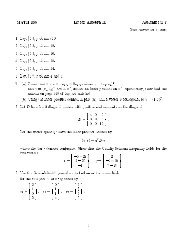
Preliminaries: Semidefinite Programming (SDP)Max-Cut Problem (MC); Simplest of Hard ProblemsSDP from General Quadratic Approximations (QQP)Quadratic Assignment Problem, (QAP);Hardest of Hard ProblemsThe Sensor Network Localization, SNL, ProblemSTRENGTH of Relaxaton; Theory and EmpiricalSDP Relaxation of Max-Cut Problem, (MC)Max-Cut Problemundirected, complete, graph G = (V, E), |V| = n, with edgeweights w ij ; divide nodes into two sets to maximize the sum ofweights of cut edges.A Maximum Cut

23Preliminaries: Semidefinite Programming (SDP)Max-Cut Problem (MC); Simplest of Hard ProblemsSDP from General Quadratic Approximations (QQP)Quadratic Assignment Problem, (QAP);Hardest of Hard ProblemsThe Sensor Network Localization, SNL, ProblemSTRENGTH of Relaxaton; Theory and EmpiricalQuadratic-Quadratic (QQP) Model for MCQuadratic Model of MC with Integer Constraintsmax 1 ∑2 i

Preliminaries: Semidefinite Programming (SDP)Max-Cut Problem (MC); Simplest of Hard ProblemsSDP from General Quadratic Approximations (QQP)Quadratic Assignment Problem, (QAP);Hardest of Hard ProblemsThe Sensor Network Localization, SNL, ProblemSTRENGTH of Relaxaton; Theory and EmpiricalSDP Relaxation; use commutativity trace AB = trace BADirect Relaxation(4) p ∗ := max{x T Lx : x ∈ {±1} n}Replace x ∈ {±1} n with x 2i= 1. Note thatx T Lx = trace x T Lx = trace Lxx T = trace LX, withrank-1{ }} {X = xx Talso:X ≽ 0, diag(X) = e, q(x) = trace LXRelax the hard rank-1 condition on X; get SDP relaxationThe SDP Relaxation of MCp ∗ := max{trace LX : diag(X) = e, X ≽ 0}

25Preliminaries: Semidefinite Programming (SDP)Max-Cut Problem (MC); Simplest of Hard ProblemsSDP from General Quadratic Approximations (QQP)Quadratic Assignment Problem, (QAP);Hardest of Hard ProblemsThe Sensor Network Localization, SNL, ProblemDuality for SDP Relaxation of MCPrimal-Dual Programs(PSDP)d ∗ = p ∗ := maxs.t.STRENGTH of Relaxaton; Theory and Empiricaltrace LXdiag(X) = eX ≽ 0, X ∈ S n ,diag : vector from diagonal; Diag : diagonal matrix from vector; evector of ones;(DSDP)p ∗ = d ∗ := mins.t.e T yDiag(y)−Z = LZ ≽ 0, Z ∈ S n ,Slater PointsˆX = I ≻ 0; Ẑ = L−Diag(ŷ) ≻ 0 for ŷ

26Preliminaries: Semidefinite Programming (SDP)Max-Cut Problem (MC); Simplest of Hard ProblemsSDP from General Quadratic Approximations (QQP)Quadratic Assignment Problem, (QAP);Hardest of Hard ProblemsThe Sensor Network Localization, SNL, ProblemModern Optimality FrameworkSTRENGTH of Relaxaton; Theory and Empirical(Perturbed) Overdetermined Optimality Conditions, X, Z ≻ 0⎧R d := Diag(y)−Z − L = 0 dual feas.⎪⎨RF µ (X, y, Z) = p := diag(X)−e = 0 primal feas.ZX = 0 compl. slack.⎪⎩R c := ZX −µI = 0 pert. compl. slack.ZX NOT nec. symmetricLinearization/(Gauss)-Newton Direction⎛ ⎞ ⎡ ⎤∆X Diag(∆y)−∆ZF µ ′ (X, y, Z) ⎝∆y⎠ = ⎣ diag(∆X) ⎦ = −F µ (X, y, Z)∆Z Z∆X +∆ZX

28Preliminaries: Semidefinite Programming (SDP)Max-Cut Problem (MC); Simplest of Hard ProblemsSDP from General Quadratic Approximations (QQP)Quadratic Assignment Problem, (QAP);Hardest of Hard ProblemsThe Sensor Network Localization, SNL, ProblemMATLAB CodeSTRENGTH of Relaxaton; Theory and EmpiricalInitialization: X, Z ≻ 0function [phi, X, y] = psd_ip( L);% solves: max trace(LX) s.t. X psd, diag(X) = b; b = ones(n,1)/4% min b’y s.t. Diag(y) - L psd, y unconstrained,%**input: L ... symmetric matrix%**output: phi ... optimal value of primal, phi =trace(LX)% X ... optimal primal matrix% y ... optimal dual vector% call: [phi, X, y] = psd_ip( L);%%%%%%%%%%%%%%%%%%%%%Initializationdigits = 6;% 6 significant digits of phi[n, n1] = size( L);% problem sizeb = ones( n,1 ) / 4;% any b>0 works just as wellX = diag( b);% initial primal matrix is pos. def.y = sum( abs( L))’ * 1.1; % initial y is chosen so thatZ = diag( y) - L;% initial dual slack Z is pos. def.phi = b’*y;% initial dual costspsi = L(:)’ * X( :);% and initial primal costsmu = Z( :)’ * X( :)/( 2*n); % initial complementarityiter=0;% iteration count

29Preliminaries: Semidefinite Programming (SDP)Max-Cut Problem (MC); Simplest of Hard ProblemsSDP from General Quadratic Approximations (QQP)Quadratic Assignment Problem, (QAP);Hardest of Hard ProblemsThe Sensor Network Localization, SNL, ProblemFind Search Direction/Symmetrize dXSTRENGTH of Relaxaton; Theory and EmpiricalSolve: dy; backsolve: dZ, dX ; symmetrize dXdisp([’ iter alphap alphad gap lower upper’]);while phi-psi > max([1,abs(phi)]) * 10^(-digits)iter = iter + 1;% start a new iterationZi = inv( Z);% inv(Z) is needed explicitlyZi = (Zi + Zi’)/2;dy = (Zi.*X) \ (mu * diag(Zi) - b); % solve for dydX = - Zi * diag( dy) * X + mu * Zi - X; % back substitute for dXdX = ( dX + dX’)/2; % symmetrize

Preliminaries: Semidefinite Programming (SDP)Max-Cut Problem (MC); Simplest of Hard ProblemsSDP from General Quadratic Approximations (QQP)Quadratic Assignment Problem, (QAP);Hardest of Hard ProblemsThe Sensor Network Localization, SNL, ProblemSTRENGTH of Relaxaton; Theory and EmpiricalLine Search to Stay Interior; and UpdateBacktrack to keep X, Z ≻ 0; Update X, y, Z% line search on primalalphap = 1;% initial steplength[dummy,posdef] = chol( X + alphap * dX ); % test if pos.defwhile posdef > 0,alphap = alphap * .8;[dummy,posdef] = chol( X + alphap * dX );end;if alphap < 1, alphap = alphap * .95; end; % stay away from boundary% line search on dual; dZ is handled implicitly: dZ = diag( dy);alphad = 1;[dummy,posdef] = chol( Z + alphad * diag(dy) );while posdef > 0;alphad = alphad * .8;[dummy,posdef] = chol( Z + alphad * diag(dy) );end;if alphad < 1, alphad = alphad * .95; end;% updateX = X + alphap * dX;y = y + alphad * dy;Z = Z + alphad * diag(dy);mu = X( :)’ * Z( :) / (2*n);if alphap + alphad > 1.8, mu = mu/2; end; % speed up for long stepsphi = b’ * y; psi = L( :)’ * X( :);% display current iterationdisp([ iter alphap alphad (phi-psi) psi phi ]);30

31Preliminaries: Semidefinite Programming (SDP)Max-Cut Problem (MC); Simplest of Hard ProblemsSDP from General Quadratic Approximations (QQP)Quadratic Assignment Problem, (QAP);Hardest of Hard ProblemsThe Sensor Network Localization, SNL, ProblemSuccess of SDP Relaxation of MCSTRENGTH of Relaxaton; Theory and EmpiricalGoemans-Williamson .878 approx. algor. for MCMC is one of Karp’s NP-complete problems (APX-hard);G-W ’94 showed (with nonnegative weights on edges):.87856(bnd SDP ) ≤ optvalue MC ≤ bnd SDPExtensions/NumericsThis result has been extended (e.g. Nesterov/97) to moregeneral quadratic functions to obtain a π 2 guaranteeIn practice, the strength of the bound is much tighter; largeproblems can be solved (many authors).

32Preliminaries: Semidefinite Programming (SDP)Max-Cut Problem (MC); Simplest of Hard ProblemsSDP from General Quadratic Approximations (QQP)Quadratic Assignment Problem, (QAP);Hardest of Hard ProblemsThe Sensor Network Localization, SNL, ProblemSDP Relaxation is EQUIVALENT to Lagrangian RelaxationSDP arise from general quadratic approximations?General Quadratic ApproximationsApproximations from quadratic functions are stronger than fromlinear functions. E.g.x ∈ {±1} iff x 2 = 1 x ∈ {0, 1} iff x 2 − x = 0QQPsLetq i (y) = 1 2 y T Q i y + y T b i + c i , y ∈ R n(QQP)q ∗ = min q 0 (y)s.t. q i (y) ≤ 0i = 1,...m

Preliminaries: Semidefinite Programming (SDP)Max-Cut Problem (MC); Simplest of Hard ProblemsSDP from General Quadratic Approximations (QQP)Quadratic Assignment Problem, (QAP);Hardest of Hard ProblemsThe Sensor Network Localization, SNL, ProblemLagrangian RelaxationSDP Relaxation is EQUIVALENT to Lagrangian RelaxationLagrangian; x Lagrange multiplier vectorL(y, x) = q 0 (y)+ ∑ mi=1 x iq i (y)or equivalently (combine quad./lin. terms)L(y, x) = 1 2 y T (Q 0 + ∑ mi=1 x iQ i )y+y T (b 0 + ∑ mi=1 x ib i )+(c 0 + ∑ mi=1 x ic i )Weak DualityUse hidden constraintsd ∗ = maxminx≥0 yL(y, x) ≤ q ∗ = min33ymax L(y, x)x≥0

34Preliminaries: Semidefinite Programming (SDP)Max-Cut Problem (MC); Simplest of Hard ProblemsSDP from General Quadratic Approximations (QQP)Quadratic Assignment Problem, (QAP);Hardest of Hard ProblemsThe Sensor Network Localization, SNL, ProblemHomogenizationSDP Relaxation is EQUIVALENT to Lagrangian RelaxationHomogenize the Lagrangianmultiply linear term by new variable y 0 :y 0 y T (b 0 + ∑ mi=1 x ib i ), y0 2 = 1use: strong duality for TRS; hidden SDP constraintsd ∗ = max min y L(y, x)x≥0= max min 1x≥0 y0 2=1 2 y T (Q 0 + ∑ mi=1 x iQ i )y + ty02= max minx≥0,t y+y 0 y T (b 0 + ∑ mi=1 x ib i )+(c 0 + ∑ mi=1 x ic i )−t12 y T (Q 0 + ∑ mi=1 x iQ i )y + ty02+y 0 y T (b 0 + ∑ mi=1 x ib i )+(c 0 + ∑ mi=1 x ic i )−t

NOTE: There is NO hidden constraint needed in convex case;e.g. if all q i are convex.35Preliminaries: Semidefinite Programming (SDP)Max-Cut Problem (MC); Simplest of Hard ProblemsSDP from General Quadratic Approximations (QQP)Quadratic Assignment Problem, (QAP);Hardest of Hard ProblemsThe Sensor Network Localization, SNL, ProblemSDP Relaxation is EQUIVALENT to Lagrangian RelaxationHidden SDP Constraint in Lagrangian DualHessian is ≽ 0( ) 0 bTB := 0,b 0 Q 0( [ ∑ t tmA := − ∑ i=1x)x ibiT ]mi=1 x ∑ mib i i=1 x , : R m+1 → S n+1iQ iand the SDP constraint( tB −Ax)≽ 0.

Preliminaries: Semidefinite Programming (SDP)Max-Cut Problem (MC); Simplest of Hard ProblemsSDP from General Quadratic Approximations (QQP)Quadratic Assignment Problem, (QAP);Hardest of Hard ProblemsThe Sensor Network Localization, SNL, ProblemSDP Relaxation is EQUIVALENT to Lagrangian RelaxationLagrangian Relaxation and Equivalent SDPDual-Primal ProgramsLagrangian Relaxation is equivalent to SDP (with c 0 = 0)(DSDP)d ∗ = sups.t.−t + ∑ m( i=1 )x ic itA ≼ Bxx ∈ R m , t ∈ RAs in LP, Dual of Dual; Use Opt. Strategy of Competing Playerd ∗ ≤ p ∗ := inf trace(BY) −1(DD)s.t. A ∗ Y =cY ≽ 0.36

37Preliminaries: Semidefinite Programming (SDP)Max-Cut Problem (MC); Simplest of Hard ProblemsSDP from General Quadratic Approximations (QQP)Quadratic Assignment Problem, (QAP);Hardest of Hard ProblemsThe Sensor Network Localization, SNL, ProblemQQP Model of QAPQAP with ADDITIONAL REDUNDANT ConstraintsQuadratic Assignment Problem, (QAP)QAP Problemn facilities i, l, A il flow or weight;n locations j, k, B jk distances;C ij location costsn ≥ 16 considered hard; SDP provides strong (thoughexpensive) bounds/1998;Nugent n = 30 solved for first time using weakened SDPrelaxation on computational grids (CONDOR)/2002;Exploit group symmetry in SDP relaxation of QAP; majoradvance in size and efficiency/2007

38Preliminaries: Semidefinite Programming (SDP)Max-Cut Problem (MC); Simplest of Hard ProblemsSDP from General Quadratic Approximations (QQP)Quadratic Assignment Problem, (QAP);Hardest of Hard ProblemsThe Sensor Network Localization, SNL, ProblemQAP FormulationQQP Model of QAPQAP with ADDITIONAL REDUNDANT ConstraintsQAP Applicationsdesigning of facility layouts; VLSI design (location of moduleson chips); campus planning; scheduling; processcommunication; turbine balancing; typewriter keyboard design;many more . . .QAP Trace Formulation/Model(QAP) µ ∗ := minX∈Π trace AXBX T − 2CX TA, B, C ∈ M n ; Π set of permutaion matrices.

39Preliminaries: Semidefinite Programming (SDP)Max-Cut Problem (MC); Simplest of Hard ProblemsSDP from General Quadratic Approximations (QQP)Quadratic Assignment Problem, (QAP);Hardest of Hard ProblemsThe Sensor Network Localization, SNL, ProblemQQP Model of QAPQAP with ADDITIONAL REDUNDANT ConstraintsQuadratic Assignment Problem, (QAP)Permutation MatricesΠ = {n×n : (0, 1), row/col sums 1}= { X ∈ M n : X ◦ X = X, Xe = X T e = e }= { X ∈ M n : X T X = I, Xe = X T e = e, X ≥ 0 }= { X ∈ M n : X T X = XX T = I, Xe = X T e = e,X ◦ X = X, X ≥ 0}QQP Model of QAP/Add Redundant Constraints(QAP E )µ ∗ := min trace AXBX T − 2CX Ts.t. XX T = I, X T X = IXe = X T e = eXij 2 − X ij = 0, ∀i, j.

Preliminaries: Semidefinite Programming (SDP)Max-Cut Problem (MC); Simplest of Hard ProblemsSDP from General Quadratic Approximations (QQP)Quadratic Assignment Problem, (QAP);Hardest of Hard ProblemsThe Sensor Network Localization, SNL, ProblemLagrangian Relaxation of QAPQQP Model of QAPQAP with ADDITIONAL REDUNDANT ConstraintsFind SDP relaxation of QAP by taking dual of dual(ignore Xe = X T e = e for now)• Add (0, 1)-constraints to objective function; use Lagrangemultipliers W ijµ O = min max trace AXBX T − 2CX T + ∑XX T ij W ij(Xij 2 − X ij )=I WX T X=Ihomogenize obj. fn; multiply by a constrained scalar x 0µ O ≥ µ R = maxWminXX T =X T X=Ix 2 0 =140trace [ AXBX T + W(X ◦ X) T−x 0 (2C + W)X T] .

Preliminaries: Semidefinite Programming (SDP)Max-Cut Problem (MC); Simplest of Hard ProblemsSDP from General Quadratic Approximations (QQP)Quadratic Assignment Problem, (QAP);Hardest of Hard ProblemsThe Sensor Network Localization, SNL, ProblemLagrangian Relaxation/DualQQP Model of QAPQAP with ADDITIONAL REDUNDANT ConstraintsGrouping: quadratic, linear, constant termsLagrange multiplier w 0 for constraint on x 0 ; Lagrange multipliersS b for XX T = I, S o for X T X = Iµ O ≥ µ R := maxWmin trace [ AXBX T + W(X ◦ X) T + w 0 x02 X, x 0+S b XX T + S o X T X ]−trace x 0 (2C + W)X T−w 0 − trace S b − trace S o .

Preliminaries: Semidefinite Programming (SDP)Max-Cut Problem (MC); Simplest of Hard ProblemsSDP from General Quadratic Approximations (QQP)Quadratic Assignment Problem, (QAP);Hardest of Hard ProblemsThe Sensor Network Localization, SNL, ProblemLagrangian Relaxation/DualQQP Model of QAPQAP with ADDITIONAL REDUNDANT ConstraintsVectorize Xdefine x := vec X, y T := (x 0 , x T ) and w T := (w 0 , vec W T )µ R = max minW yy T [ L Q + Arrow(w)+B 0 Diag(S b )+O 0 Diag(S o ) ] y−w 0 − trace S b − trace S o

43Preliminaries: Semidefinite Programming (SDP)Max-Cut Problem (MC); Simplest of Hard ProblemsSDP from General Quadratic Approximations (QQP)Quadratic Assignment Problem, (QAP);Hardest of Hard ProblemsThe Sensor Network Localization, SNL, ProblemLinear TransformationsQQP Model of QAPQAP with ADDITIONAL REDUNDANT Constraintsand[L Q :=0 −vec(C) T−vec(C) B ⊗ A[Arrow(w) :=B 0 Diag(S) :=O 0 Diag(S) :=], (n 2 + 1)×(n 2 + 1)w 0 − 1 2 w T ]1:n 2− 1 2 w 1:n 2 Diag (w 1:n 2) ,[ ]0 00 I ⊗ S b[ 0 00 S o ⊗ I].

Preliminaries: Semidefinite Programming (SDP)Max-Cut Problem (MC); Simplest of Hard ProblemsSDP from General Quadratic Approximations (QQP)Quadratic Assignment Problem, (QAP);Hardest of Hard ProblemsThe Sensor Network Localization, SNL, ProblemDual of DualQQP Model of QAPQAP with ADDITIONAL REDUNDANT ConstraintsHidden Semidefinite Constraint Yields the Equivalend SDP(D O )maxs.t.−w 0 − trace S b − trace S oL Q + Arrow(w)+B 0 Diag(S b )+O 0 Diag(S o ) ≽ 0,dual of this dual yields the semidefinite relaxation; Y ≽ 0 is(n 2 + 1)×(n 2 + 1), the dual matrix variable(SDP O )min trace L Q Ys.t. b 0 diag(Y) = I o 0 diag(Y) = Iarrow(Y) = e 0 Y ≽ 0

45Preliminaries: Semidefinite Programming (SDP)Max-Cut Problem (MC); Simplest of Hard ProblemsSDP from General Quadratic Approximations (QQP)Quadratic Assignment Problem, (QAP);Hardest of Hard ProblemsThe Sensor Network Localization, SNL, ProblemLagrangian Relaxation/DualQQP Model of QAPQAP with ADDITIONAL REDUNDANT ConstraintsAdjoint Operatorsarrow(Y) := diag(Y)−(0,(Y 0,1:n 2) T .b 0 diag(Y) :=n∑k=1Y (k−1)n+1:kn,(k−1)n+1:kn[o 0 diag(Y)] ij := trace Y (i−1)n+1:in,(j−1)n+1:jn

46Preliminaries: Semidefinite Programming (SDP)Max-Cut Problem (MC); Simplest of Hard ProblemsSDP from General Quadratic Approximations (QQP)Quadratic Assignment Problem, (QAP);Hardest of Hard ProblemsThe Sensor Network Localization, SNL, ProblemDirect Approach to SDP RelaxationQQP Model of QAPQAP with ADDITIONAL REDUNDANT ConstraintsVectorize Permutation MatrixX ∈ Π; x = vec(X), c = vec(C).q(X) = trace AXBX T − 2CX T= x T (B ⊗ A)x − 2c T x= trace xx T (B ⊗ A)−2c T x= trace L Q Y X ,[ ] 1 xTY X :=x xx T

Preliminaries: Semidefinite Programming (SDP)Max-Cut Problem (MC); Simplest of Hard ProblemsSDP from General Quadratic Approximations (QQP)Quadratic Assignment Problem, (QAP);Hardest of Hard ProblemsThe Sensor Network Localization, SNL, ProblemLoss of Slater CQQQP Model of QAPQAP with ADDITIONAL REDUNDANT ConstraintsCommentsAfter adding the row/column sum constraints Xe = X T e = e,we get that Slater’s CQ fails; but we can explicitly regularize, i.e.find the smallest face/minimal cone. the SDP relaxationprovides strong bounds, but expensive. Exploit groupsymmetries/special structure.

48Preliminaries: Semidefinite Programming (SDP)Max-Cut Problem (MC); Simplest of Hard ProblemsSDP from General Quadratic Approximations (QQP)Quadratic Assignment Problem, (QAP);Hardest of Hard ProblemsThe Sensor Network Localization, SNL, ProblemEXPLOIT DEGENERACY and FACIAL StructureSensor Network Localization, SNL, (Krislock and W.)Wireless Sensor Networkn ad hoc wireless sensors (nodes) to locate in R r ,(r is embedding dimension;sensors p i ∈ R r , i ∈ V := 1,...,n)m of the sensors are anchors, p i , i = n− m+1,...,n)(e.g. using GPS)pairwise distances known within radio range R,D ij = ‖p i − p j ‖ 2 , ij ∈ ECurrent Techniques: Nearest, Weighted, SDP Approx.min Y≽0,Y∈Ω ‖H ◦(K(Y)−D)‖SDP program is: Expensive/low accuracy/implicitly highlydegenerate (cliques restrict ranks of feasible Y s)

49Preliminaries: Semidefinite Programming (SDP)Max-Cut Problem (MC); Simplest of Hard ProblemsSDP from General Quadratic Approximations (QQP)Quadratic Assignment Problem, (QAP);Hardest of Hard ProblemsThe Sensor Network Localization, SNL, ProblemApplicationsEXPLOIT DEGENERACY and FACIAL StructureTracking Humans/Animals/Equipmentmonitoring: natural habitat; earthquakes and volcanos;weather and ocean currents.military, tracking of goods, vehicle positions, surveillance,(where open-air positioning is not feasible), randomdeployment in inaccessible terrains or disaster reliefoperations

Preliminaries: Semidefinite Programming (SDP)Max-Cut Problem (MC); Simplest of Hard ProblemsSDP from General Quadratic Approximations (QQP)Quadratic Assignment Problem, (QAP);Hardest of Hard ProblemsThe Sensor Network Localization, SNL, ProblemEXPLOIT DEGENERACY and FACIAL StructureUnderlying Graph Realization/Partial EDMGraph G = (V ,E ,ω)node set V = {1,...,n}edge set (i, j) ∈ E ; ω ij = ‖p i − p j ‖ 2 known approximatelyThe anchors form a clique (complete subgraph)Realization of G in R r : a mapping of node v i → p i ∈ R rwith squared distances given by ω.Corresponding Partial Euclidean Distance Matrix, EDM{ d2D ij = ijif (i, j) ∈ E0 otherwise,d 2ij= ω ij are known squared Euclidean distances betweensensors p i , p j ; anchors correspond to a clique.50

Preliminaries: Semidefinite Programming (SDP)Max-Cut Problem (MC); Simplest of Hard ProblemsSDP from General Quadratic Approximations (QQP)Quadratic Assignment Problem, (QAP);Hardest of Hard ProblemsThe Sensor Network Localization, SNL, ProblemEXPLOIT DEGENERACY and FACIAL StructureSensor Localization Problem/Partial EDMSensors ◦ and Anchors109Initial position of pointssensorsanchorssens−anch8765432100 1 2 3 4 5 6 7 8 9 10# sensors n = 300, # anchors m = 9, radio range R = 1.251

Preliminaries: Semidefinite Programming (SDP)Max-Cut Problem (MC); Simplest of Hard ProblemsSDP from General Quadratic Approximations (QQP)Quadratic Assignment Problem, (QAP);Hardest of Hard ProblemsThe Sensor Network Localization, SNL, ProblemFurther NotationEXPLOIT DEGENERACY and FACIAL StructureMatrix with Fixed Principal SubmatrixFor Y ∈ S n , α ⊆ {1,..., n}: Y[α] denotes principal submatrixformed from rows & cols with indices α.Sets with Fixed Principal SubmatricesIf |α| = k and Ȳ ∈ Sk , then:S n (α, Ȳ) := { Y ∈ S k : Y[α] = Ȳ} ,S+ n (α, Ȳ) := { Y ∈ S+ k : Y[α] = Ȳ}i.e. the subset of matrices Y ∈ S k (Y ∈ S+ k ) with principalsubmatrix Y[α] fixed to Ȳ . 52

53Preliminaries: Semidefinite Programming (SDP)Max-Cut Problem (MC); Simplest of Hard ProblemsSDP from General Quadratic Approximations (QQP)Quadratic Assignment Problem, (QAP);Hardest of Hard ProblemsThe Sensor Network Localization, SNL, ProblemEXPLOIT DEGENERACY and FACIAL StructureSNL Connection to SDP (Lin. Trans., Adjoints)v = diag(S) ∈ R n , S = Diag(v) ∈ S ndiag = Diag ∗ (adjoint)for B ∈ S n , offDiag(B) := B − Diag(diag(B))D = K(B) ∈ E n , B = K † (D) ∈ S n ∩S CLet P T = [ p 1 p 2 ... p n]∈ M r×n ;B := PP T ∈ S n ; D ∈ E n be corresponding EDM .(from S n ) K(B) := D e (B)−2B:= diag(B) e T + e diag(B) T − 2B( ) n= pi T p i + pj T p j − 2pi T p ji,j=1= ( ‖p i − p j ‖ 2 2) ni,j=1= D (to E n ).

54Preliminaries: Semidefinite Programming (SDP)Max-Cut Problem (MC); Simplest of Hard ProblemsSDP from General Quadratic Approximations (QQP)Quadratic Assignment Problem, (QAP);Hardest of Hard ProblemsThe Sensor Network Localization, SNL, ProblemK : S n + ∩S C → E nEXPLOIT DEGENERACY and FACIAL StructureLinear Transformations: D v (B),K(B),T (D)allow: D v (B) := diag(B) v T + v diag(B) T ;D v (y) := yv T + vy Tadjoint K ∗ (D) = 2(Diag(De)−D).K is 1−1, onto between centered and hollow subspaces:S C := {B ∈ S n : Be = 0};S H := {D ∈ S n : diag(D) = 0} = R(offDiag)J := I − 1 n eeT (orthogonal projection onto M := {e} ⊥ );T (D) := − 1 2 JoffDiag(D)J(= K † (D))

55Preliminaries: Semidefinite Programming (SDP)Max-Cut Problem (MC); Simplest of Hard ProblemsSDP from General Quadratic Approximations (QQP)Quadratic Assignment Problem, (QAP);Hardest of Hard ProblemsThe Sensor Network Localization, SNL, ProblemProperties of Linear TransformationsEXPLOIT DEGENERACY and FACIAL StructureK,T , Diag,D eR(K) = S H ; N (K) = R(D e );R(K ∗ ) = R(T ) = S C ;N (K ∗ ) = N (T ) = R(Diag);S n = S H ⊕R(Diag) = S C ⊕R(D e ).T (E n ) = S n +∩S C and K(S n +∩S C ) = E n .

56Preliminaries: Semidefinite Programming (SDP)Max-Cut Problem (MC); Simplest of Hard ProblemsSDP from General Quadratic Approximations (QQP)Quadratic Assignment Problem, (QAP);Hardest of Hard ProblemsThe Sensor Network Localization, SNL, ProblemSingle Clique/Facial ReductionEXPLOIT DEGENERACY and FACIAL Structure¯D ∈ E k , α ⊆ 1:n, |α| = kDefine E n (α, ¯D) := { D ∈ E n : D[α] = ¯D } .Given ¯D; find a corresponding B ≽ 0; find the correspondingface; find the corresponding subspace.

Note that we add 1 √ke to represent N (K); then we use V toeliminate e to recover centered face.57Preliminaries: Semidefinite Programming (SDP)Max-Cut Problem (MC); Simplest of Hard ProblemsSDP from General Quadratic Approximations (QQP)Quadratic Assignment Problem, (QAP);Hardest of Hard ProblemsThe Sensor Network Localization, SNL, ProblemEXPLOIT DEGENERACY and FACIAL StructureBasic Theorem for Single Clique/Facial ReductionTHEOREM 1: Single Clique ReductionLet ¯D := D[1:k] ∈ E k , k < n, with embedding dimension t ≤ r,and B := K † (¯D) = ŪBSŪT B , where ŪB ∈ M k×t ], ŪT B ŪB = I t , andS ∈ S++. t 1Furthermore, let U B :=[ŪB √k e ∈ M k×(t+1) ,[ ]UB 0[ ]UU :=, and let VT e∈ M n−k+t+1 be0 I ‖U T e‖n−korthogonal. Then:faceK †( E n (1:k, ¯D) ) (= US+ n−k+t+1 U)∩S T C= (UV)S+ n−k+t (UV) T

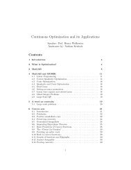
For each clique |α| = k, we get a corresponding face/subspace(k × r matrix) representation. We now see how to handle twocliques, α 1 ,α 2 , that intersect.58Preliminaries: Semidefinite Programming (SDP)Max-Cut Problem (MC); Simplest of Hard ProblemsSDP from General Quadratic Approximations (QQP)Quadratic Assignment Problem, (QAP);Hardest of Hard ProblemsThe Sensor Network Localization, SNL, ProblemEXPLOIT DEGENERACY and FACIAL StructurePositive Integers for Intersecting CliquesTwo Intersection Sets, α 1 ,α 2 .α 1α 2¯k 1¯k 2¯k3

59Preliminaries: Semidefinite Programming (SDP)Max-Cut Problem (MC); Simplest of Hard ProblemsSDP from General Quadratic Approximations (QQP)Quadratic Assignment Problem, (QAP);Hardest of Hard ProblemsThe Sensor Network Localization, SNL, ProblemEXPLOIT DEGENERACY and FACIAL StructureTwo (Intersecting) Clique Reduction/Subsp. Repres.THEOREM 2: Clique Intersection Reduction/Subsp. Repres.α 1 := 1:(¯k 1 + ¯k 2 ), α 2 := (¯k 1 + 1):(¯k 1 + ¯k 2 + ¯k 3 ) ⊆ 1:n,k 1 := |α 1 | = ¯k 1 + ¯k 2 , k 2 := |α 2 | = ¯k 2 + ¯k 3 ,k := ¯k 1 + ¯k 2 + ¯k 3 .For i = 1, 2, let ¯D i := D[α i ] ∈ E k i, with embedding dimension t i ,and B i := K † (¯D i ) = ŪiS i Ūi T , where Ūi ∈ M k i×t i, ŪT iŪ i = I ti ,and S i ∈ S t i++ . Furthermore, for i = 1, 2, let1[ŪiU i :=√ e ]ki∈ M k i×(t i +1) , and let Ū ∈ M k×(t+1) satisfy([ ])I¯k10, with0 U ŪT Ū = I t+12([ ])R(Ū) = RU1 0∩R0 I¯k3cont. . .

60Preliminaries: Semidefinite Programming (SDP)Max-Cut Problem (MC); Simplest of Hard ProblemsSDP from General Quadratic Approximations (QQP)Quadratic Assignment Problem, (QAP);Hardest of Hard ProblemsThe Sensor Network Localization, SNL, ProblemEXPLOIT DEGENERACY and FACIAL StructureTwo (Intersecting) Clique Reduction, cont. . .THEOREM 2 Nonsing. Clique Inters. cont. . .cont. . . with([ ])R(Ū) = RU1 0∩R0 I¯k3[Ū ] 0let U := ∈ M n×(n−k+t+1) and let0 I[ ] n−kV ∈ M n−k+t+1 be orthogonal. ThenU T e‖U T e‖⋂ 2i=1 faceK†( E n (α i , ¯D i ) ) =([I¯k100 U 2]), with ŪT Ū = I t+1 ,(US n−k+t+1+ U T )∩S C= (UV)S n−k+t+ (UV) TBasic work: find Ū to repres. inters. of 2 subspaces.

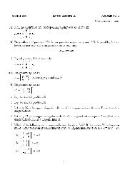
Completion: missing distances can be recovered if desired.61Preliminaries: Semidefinite Programming (SDP)Max-Cut Problem (MC); Simplest of Hard ProblemsSDP from General Quadratic Approximations (QQP)Quadratic Assignment Problem, (QAP);Hardest of Hard ProblemsThe Sensor Network Localization, SNL, ProblemEXPLOIT DEGENERACY and FACIAL StructureTwo (Intersecting) Clique Reduction Figure

62Preliminaries: Semidefinite Programming (SDP)Max-Cut Problem (MC); Simplest of Hard ProblemsSDP from General Quadratic Approximations (QQP)Quadratic Assignment Problem, (QAP);Hardest of Hard ProblemsThe Sensor Network Localization, SNL, ProblemEXPLOIT DEGENERACY and FACIAL StructureTwo (Intersecting) Clique Explicit CompletionCOR. Intersection with Embedding Dim. r/CompletionHypotheses of Theorem 2 holds. Let ¯D i := D[α i ] ∈ E k i, fori = 1, 2, β ⊆ α 1 ∩α 2 ,γ := α 1 ∪α 2 , ¯D := D[β], B :=K † (¯D), Ū β := Ū(β,:), where Ū ∈ M k×(t+1) satisfiesintersection equation of Theorem 2. Let[¯VŪ T e‖ŪT e‖be orthogonal. Let Z := (JŪβ¯V) † B((JŪβ¯V) † ) T . If the]∈ M t+1embedding dimension for ¯D is r, THEN t = r in Theorem 2, andZ ∈ S+ r is the unique solution of the equation(JŪβ¯V)Z(JŪβ¯V) T = B, and the exact completion isD[γ] = K ( (Ū¯V)Z(Ū¯V) T) .

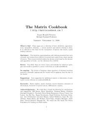
63Preliminaries: Semidefinite Programming (SDP)Max-Cut Problem (MC); Simplest of Hard ProblemsSDP from General Quadratic Approximations (QQP)Quadratic Assignment Problem, (QAP);Hardest of Hard ProblemsThe Sensor Network Localization, SNL, ProblemEXPLOIT DEGENERACY and FACIAL Structure2 (Inters.) Clique Reduction/Singular CaseTwo (Intersecting) Clique Reduction/Singular CaseC iC jUse R as lower bound in singular/nonrigid case.

64Preliminaries: Semidefinite Programming (SDP)Max-Cut Problem (MC); Simplest of Hard ProblemsSDP from General Quadratic Approximations (QQP)Quadratic Assignment Problem, (QAP);Hardest of Hard ProblemsThe Sensor Network Localization, SNL, ProblemAlgorithmEXPLOIT DEGENERACY and FACIAL StructureInitializeC i := { j : (D p ) ij < (R/2) 2} , for i = 1,...,nIterateFinalizeFor |C i ∩ C j | ≥ r + 1, do Rigid Clique UnionFor |C i ∩N (j)| ≥ r + 1, do Rigid Node AbsorptionFor |C i ∩ C j | = r, do Non-Rigid Clique Union (lower bnds)For |C i ∩N (j)| = r, do Non-Rigid Node Absorp. (lowerbnds)When ∃ a clique containing all anchors, use computed facialrepresentation and positions of anchors to solve for X

65Preliminaries: Semidefinite Programming (SDP)Max-Cut Problem (MC); Simplest of Hard ProblemsSDP from General Quadratic Approximations (QQP)Quadratic Assignment Problem, (QAP);Hardest of Hard ProblemsThe Sensor Network Localization, SNL, ProblemAlgorithmEXPLOIT DEGENERACY and FACIAL StructureClique UnionNode AbsorptionRigidNon-rigidC iCiC jj

66Preliminaries: Semidefinite Programming (SDP)Max-Cut Problem (MC); Simplest of Hard ProblemsSDP from General Quadratic Approximations (QQP)Quadratic Assignment Problem, (QAP);Hardest of Hard ProblemsThe Sensor Network Localization, SNL, ProblemEXPLOIT DEGENERACY and FACIAL StructureResults - Data for Random Noisless Problems2.16 GHz Intel Core 2 Duo, 2 GB of RAMDimension r = 2Square region: [0, 1]×[0, 1]m = 9 anchorsUsing only Rigid Clique Union and Rigid Node AbsorptionError measure: Root Mean Square DeviationRMSD =(1nn∑i=1‖p i − p truei ‖ 2 ) 1/2

67Preliminaries: Semidefinite Programming (SDP)Max-Cut Problem (MC); Simplest of Hard ProblemsSDP from General Quadratic Approximations (QQP)Quadratic Assignment Problem, (QAP);Hardest of Hard ProblemsThe Sensor Network Localization, SNL, ProblemEXPLOIT DEGENERACY and FACIAL StructureResults - Large n (SDP size O(n 2 ))n # of Sensors Locatedn # sensors \ R 0.07 0.06 0.05 0.042000 2000 2000 1956 13746000 6000 6000 6000 600010000 10000 10000 10000 10000CPU Seconds# sensors \ R 0.07 0.06 0.05 0.042000 1 1 1 36000 5 5 4 410000 10 10 9 8RMSD (over located sensors)n # sensors \ R 0.07 0.06 0.05 0.042000 4e−16 5e−16 6e−16 3e−166000 4e−16 4e−16 3e−16 3e−1610000 3e−16 5e−16 4e−16 4e−16

68Preliminaries: Semidefinite Programming (SDP)Max-Cut Problem (MC); Simplest of Hard ProblemsSDP from General Quadratic Approximations (QQP)Quadratic Assignment Problem, (QAP);Hardest of Hard ProblemsThe Sensor Network Localization, SNL, ProblemResults - N Huge SDPs SolvedEXPLOIT DEGENERACY and FACIAL StructureLarge-Scale Problems# sensors # anchors radio range RMSD Time20000 9 .025 5e−16 25s40000 9 .02 8e−16 1m 23s60000 9 .015 5e−16 3m 13s100000 9 .01 6e−16 9m 8s( nSize of SDPs Solved: N = (# vrbls)2)E n (density of G) = πR 2 ; M = E n (|E|) = πR 2 N (# constraints)Size of SDP Problems:M = [ 3, 078, 915 12, 315, 351 27, 709, 309 76, 969, 790 ]N = 10 9[ 0.2000 0.8000 1.8000 5.0000 ]

69Preliminaries: Semidefinite Programming (SDP)Max-Cut Problem (MC); Simplest of Hard ProblemsSDP from General Quadratic Approximations (QQP)Quadratic Assignment Problem, (QAP);Hardest of Hard ProblemsThe Sensor Network Localization, SNL, ProblemSummaryEXPLOIT DEGENERACY and FACIAL StructureMany hard (combinatorial) problems can be modelledusing quadratic objectives and constraints, QQPs.QQPs are generally NP-hard problems. But, theLagrangian relaxation can be solved efficiently using theequivalent SDP (relaxation).The special structure of the SDP relaxations can beexploited in order to get efficient solutions for large scaleproblems.Many SDP relaxations of combinatorial problems aredegenerate. But, this degeneracy can be exploited. Inparticular, the SDP relaxation of SNL is highly (implicitly)degenerate. This degeneracy allows for a fast, accuratesolution technique.

70Preliminaries: Semidefinite Programming (SDP)Max-Cut Problem (MC); Simplest of Hard ProblemsSDP from General Quadratic Approximations (QQP)Quadratic Assignment Problem, (QAP);Hardest of Hard ProblemsThe Sensor Network Localization, SNL, ProblemThanks for your attention!EXPLOIT DEGENERACY and FACIAL StructureSemidefinite ProgrammingApplications and ImplementationsHenry WolkowiczDept. of Combinatorics and OptimizationUniversity of WaterlooCORS/MOPGPNiagara Falls, June 11, 2012