2328 Phys. Fluids, Vol. 15, No. 8, August 2003 Sheikhi et al.FIG. 2. Cross-stream variation <strong>of</strong> the Reynoldsaveragedvalues <strong>of</strong> at t34.3: a N E 40, b E/2.ber <strong>of</strong> successive vortex pairings and u is the wavelength <strong>of</strong>the most unstable mode corresponding to the mean streamwisevelocity pr<strong>of</strong>ile imposed at the initial time. The flowvariables are normalized with respect to the half initial vorticitythickness, L r v (t0)/2 ( v U/u L /y max ,where u L is the Reynolds averaged value <strong>of</strong> the <strong>filtered</strong>streamwise velocity and U is the velocity difference acrossthe layer. The reference velocity is U r U/2.All 2D <strong>simulation</strong>s are conducted <strong>for</strong> 0xL, and2L/3y2L/3. The <strong>for</strong>mation <strong>of</strong> <strong>large</strong> scale structures isfacilitated by introducing small harmonic, phase-shifted, disturbancescontaining subharmonics <strong>of</strong> the most unstablemode into the streamwise and cross-stream velocity pr<strong>of</strong>iles.For N p 1, this results in <strong>for</strong>mation <strong>of</strong> two <strong>large</strong> vortices andone subsequent pairing <strong>of</strong> these vortices. The 3D <strong>simulation</strong>sare conducted <strong>for</strong> a cubic box, 0xL, L/2yL/2 (0zL). The 3D field is parametrized in a procedure somewhatsimilar to that by Vreman et al. 44 The <strong>for</strong>mation <strong>of</strong> the<strong>large</strong> scale structures are expedited through eigen<strong>function</strong>based initial perturbations. 45,46 This includestwo-dimensional 42,44,47 and three-dimensional 42,48 perturbationswith a random phase shift between the 3D modes. Thisresults in the <strong>for</strong>mation <strong>of</strong> two successive vortex pairings andstrong three dimensionality.B. Numerical specificationsSimulations are conducted on equally spaced grid pointswith grid spacings xyz <strong>for</strong> 3D. All 2D <strong>simulation</strong>sare per<strong>for</strong>med on 3241 grid points. The 3D <strong>simulation</strong>sare conducted on 193 3 and 33 3 points <strong>for</strong> DNS andLES, respectively. The Reynolds number is ReU r L r /50. To filter the DNS data, a top-hat <strong>function</strong> <strong>of</strong> the <strong>for</strong>mbelow is used3Gxx G˜ x i x i ,i11, LG˜ x i x ix i x i L2 ,0, x i x i L2 .31No attempt is made to investigate the sensitivity <strong>of</strong> the resultsto the filter <strong>function</strong> 27 or the size <strong>of</strong> the filter. 49The MC particles are initially distributed throughout thecomputational region. All <strong>simulation</strong>s are per<strong>for</strong>med with auni<strong>for</strong>m ‘‘weight’’ 20 <strong>of</strong> the particles. Due to flow periodicityin the streamwise and spanwise in 3D directions, iftheparticle leaves the domain at one <strong>of</strong> these boundaries newparticles are introduced at the other boundary with the samevelocity and compositional values. In the cross-stream directions,the free-slip boundary condition is satisfied by themirror-reflection <strong>of</strong> the particles leaving through theseboundaries. The <strong>density</strong> <strong>of</strong> the MC particles is determined bythe average number <strong>of</strong> particles N E within the ensemble domain<strong>of</strong> size E E ( E ). The effects <strong>of</strong> both <strong>of</strong> theseparameters are assessed to ensure the consistency and thestatistical accuracy <strong>of</strong> the VSFDF <strong>simulation</strong>s. All results areanalyzed both ‘‘instantaneously’’ and ‘‘statistically.’’ In the<strong>for</strong>mer, the instantaneous contours snap-shots and scatterplots <strong>of</strong> the variables <strong>of</strong> interest are analyzed. In the latter,Downloaded 22 Sep 2004 to 140.121.120.39. Redistribution subject to AIP license or copyright, see http://p<strong>of</strong>.aip.org/p<strong>of</strong>/copyright.jsp
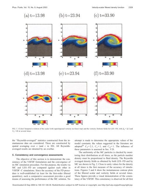
Phys. Fluids, Vol. 15, No. 8, August 2003<strong>Velocity</strong>-<strong>scalar</strong> <strong>filtered</strong> <strong>density</strong> <strong>function</strong>2329FIG. 3. Color Temporal evolution <strong>of</strong> the <strong>scalar</strong> with superimposed vorticity iso-lines top and the vorticity bottom fields <strong>for</strong> LES–FD, with E /2 andN E 40 at several times.the ‘‘Reynolds-averaged’’ statistics constructed from the instantaneousdata are considered. These are constructed byspatial averaging over x and z in 3D. All Reynoldsaveragedresults are denoted by an overbar.C. Consistency and convergence assessmentsThe objective <strong>of</strong> this section is to demonstrate the consistency<strong>of</strong> the VSFDF <strong>for</strong>mulation and the convergence <strong>of</strong>its MC <strong>simulation</strong> procedure. For this purpose, the results viaMC and LES–FD are compared against each other inVSFDF–C <strong>simulation</strong>s. Since the accuracy <strong>of</strong> the FD procedureis well-established at least <strong>for</strong> the first-order <strong>filtered</strong>quantities, such a comparative assessment provides a goodmeans <strong>of</strong> assessing the per<strong>for</strong>mance <strong>of</strong> the MC solution. Noattempt is made to determine the appropriate values <strong>of</strong> themodel constants; the values suggested in the literature areadopted 50 C 0 2.1, C 1, and C 1. The influence <strong>of</strong>these parameters is assessed in Sec. V D.The uni<strong>for</strong>mity <strong>of</strong> the MC particles is checked by monitoringtheir distributions at all times, as the particle number<strong>density</strong> must be proportional to fluid <strong>density</strong>. The Reynoldsaveraged <strong>density</strong> fields as obtained by both LES–FD and byMC are shown in Fig. 2. Close to unity values <strong>for</strong> the <strong>density</strong>at all times is the first measure <strong>of</strong> the accuracy <strong>of</strong> <strong>simulation</strong>s.Figures 3 and 4 show the instantaneous contour plots<strong>of</strong> the <strong>filtered</strong> <strong>scalar</strong> and vorticity fields at several times.These figures provide a visual demonstration <strong>of</strong> the consistency<strong>of</strong> the VSFDF. This consistency is observed <strong>for</strong> all firstDownloaded 22 Sep 2004 to 140.121.120.39. Redistribution subject to AIP license or copyright, see http://p<strong>of</strong>.aip.org/p<strong>of</strong>/copyright.jsp
- Page 4 and 5: 2324 Phys. Fluids, Vol. 15, No. 8,
- Page 7: Phys. Fluids, Vol. 15, No. 8, Augus
- Page 11 and 12: Phys. Fluids, Vol. 15, No. 8, Augus
- Page 13 and 14: Phys. Fluids, Vol. 15, No. 8, Augus
- Page 15 and 16: Phys. Fluids, Vol. 15, No. 8, Augus
- Page 17: Phys. Fluids, Vol. 15, No. 8, Augus