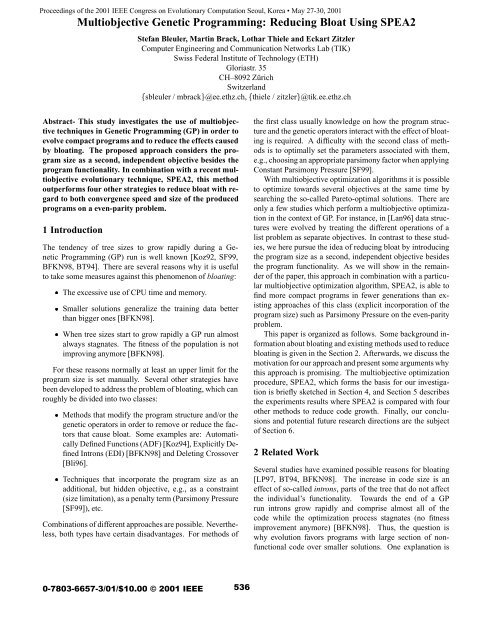
Multiobjective Genetic Programming: Reducing Bloat Using SPEA2

Multiobjective Genetic Programming: Reducing Bloat Using SPEA2Stefan Bleuler, Martin Brack, Lothar Thiele and Eckart ZitzlerComputer Engineering and Communication Networks Lab (TIK)Swiss Federal Institute of Technology (ETH)Gloriastr. 35CH–8092 ZürichSwitzerlandsbleuler / mbrack@ee.ethz.ch, thiele / zitzler@tik.ee.ethz.chAbstract- This study investigates the use of multiobjectivetechniques in Genetic Programming (GP) in order toevolve compact programs and to reduce the effects causedby bloating. The proposed approach considers the programsize as a second, independent objective besides theprogram functionality. In combination with a recent multiobjectiveevolutionary technique, SPEA2, this methodoutperforms four other strategies to reduce bloat with regardto both convergence speed and size of the producedprograms on a even-parity problem.1 IntroductionThe tendency of tree sizes to grow rapidly during a GeneticProgramming (GP) run is well known [Koz92, SF99,BFKN98, BT94]. There are several reasons why it is usefulto take some measures against this phenomenon of bloating:¯ The excessive use of CPU time and memory.¯ Smaller solutions generalize the training data betterthan bigger ones [BFKN98].¯ When tree sizes start to grow rapidly a GP run almostalways stagnates. The fitness of the population is notimproving anymore [BFKN98].For these reasons normally at least an upper limit for theprogram size is set manually. Several other strategies havebeen developed to address the problem of bloating, which canroughly be divided into two classes:¯ Methods that modify the program structure and/or thegenetic operators in order to remove or reduce the factorsthat cause bloat. Some examples are: AutomaticallyDefined Functions (ADF) [Koz94], Explicitly DefinedIntrons (EDI) [BFKN98] and Deleting Crossover[Bli96].¯ Techniques that incorporate the program size as anadditional, but hidden objective, e.g., as a constraint(size limitation), as a penalty term (Parsimony Pressure[SF99]), etc.Combinations of different approaches are possible. Nevertheless,both types have certain disadvantages. For methods ofthe first class usually knowledge on how the program structureand the genetic operators interact with the effect of bloatingis required. A difficulty with the second class of methodsis to optimally set the parameters associated with them,e.g., choosing an appropriate parsimony factor when applyingConstant Parsimony Pressure [SF99].With multiobjective optimization algorithms it is possibleto optimize towards several objectives at the same time bysearching the so-called Pareto-optimal solutions. There areonly a few studies which perform a multiobjective optimizationin the context of GP. For instance, in [Lan96] data structureswere evolved by treating the different operations of alist problem as separate objectives. In contrast to these studies,we here pursue the idea of reducing bloat by introducingthe program size as a second, independent objective besidesthe program functionality. As we will show in the remainderof the paper, this approach in combination with a particularmultiobjective optimization algorithm, SPEA2, is able tofind more compact programs in fewer generations than existingapproaches of this class (explicit incorporation of theprogram size) such as Parsimony Pressure on the even-parityproblem.This paper is organized as follows. Some background informationabout bloating and existing methods used to reducebloating is given in the Section 2. Afterwards, we discuss themotivation for our approach and present some arguments whythis approach is promising. The multiobjective optimizationprocedure, SPEA2, which forms the basis for our investigationis briefly sketched in Section 4, and Section 5 describesthe experiments results where SPEA2 is compared with fourother methods to reduce code growth. Finally, our conclusionsand potential future research directions are the subjectof Section 6.2 Related WorkSeveral studies have examined possible reasons for bloating[LP97, BT94, BFKN98]. The increase in code size is aneffect of so-called introns, parts of the tree that do not affectthe individual’s functionality. Towards the end of a GPrun introns grow rapidly and comprise almost all of thecode while the optimization process stagnates (no fitnessimprovement anymore) [BFKN98]. Thus, the question iswhy evolution favors programs with large section of nonfunctionalcode over smaller solutions. One explanation is

that GP crossover is inhomologous, i.e., it does not exchangecode fragments that have the same functionality in bothparents. Therefore crossover most often reduces the fitness ofoffspring relative to their parents by disrupting valuable codesegments or placing them in a different context. Becausecrossover points are chosen randomly within an individualthe risk of disrupting blocks of functional code can bereduced substantially by adding introns.To hinder this effect from using too much machine resourcesnormally a limit on tree depth or number of nodesis set manually. However, setting a reasonable limit is difficult.If the limit is too low, GP might not be able to find asolution. If it is too high evolution will slow down because ofthe immense resource usage and chances of finding small solutionsare very low. In the following this setup will be namedStandard GP. Here, the fitness of individual is defined asthe error of an individual’s output compared to the correctsolution. Another obvious mechanism for limiting code size is topenalize larger programs by adding a size dependent termto their fitness. This is called Constant Parsimony Pressure[Bli96, SF99]. The fitness of an individual is calculated byadding the number of edges Æ , weighted with a parsimonyfactor «, to the regular fitness: · « ¡ Æ Soule and Foster [SF99] report that in some runs ParsimonyPressure drives the entire population to the minimal possiblesize. With a higher parsimony pressure the probability of arun to suffer from this effect is increasing. This results in alower probability of finding good solutions.Another alternative is to optimize the functionality firstand the size afterwards [KM99]. The formula for the fitnessof an individual depends on its own performance. It is necessaryto set a maximal acceptable error ¯. For discrete problems¯ can be set to zero. The population is divided into twogroups:1. The individuals that have not yet reached an error equalto or smaller than ¯, get a fitness according to their error without any pressure on the size: ·½if ¯2. The fitness of an individual has reached an error that isequal to or smaller than ¯. The new fitness is calculatedusing the size Æ of individual : ½½Æ if ¯An individual with a large tree size will get a fitnessnear one while a small one will be much closer to zero.One advantage of this method is that pressure on size will nothinder GP from finding good solutions because no pressure isapplied unless the individual has already reached the aspiredperformance. In runs where no acceptable solution is foundbloating will continue. Therefore it is useful to additionallyset an upper limit on tree size. In the following we will callthis setup Two Stage according to the two stages of fitnessevaluation.Similar to this is a strategy called Adaptive ParsimonyPressure. Zhang and Mühlenbein have proposed an algorithmthat varies the parsimony factor « during the evolution[ZM95]: ´µ ´µ ·«´µ ¡ ´µ ´µ stands for the complexity of individual at generation. The complexity can be defined in several ways [ZM95].For instance as the number of nodes in a tree or as normalizedsize by dividing the individual’s size by the maximumsize in population [Bli96]. In contrast to the Two Stage strategythe fitness function does not depend on the individual’sperformance but on the best performance in the population atgeneration . The parsimony pressure used to calculate thefitness in generation is increased substantially if the best individualin the generation ½ has reached an error belowthe threshold ¯.«´µ ´½Ì ¾ ¡ ×Ø½Ì ¾ ¡´ ½µ ×Ø ´µ ×Ø ´½½µ¡ ×Ø´µif ×Ø´otherwise½µ ¯ ×Ø is the error of the best performing individual in the population.Ì denotes the size of the training set. ×Ø´µ is anestimation of the complexity of the best program, estimatedat generation ´ ½µ it is used to normalize the influence ofthe parsimony pressure. ×Ø stands for the complexity ofthe best performing individual in the population. ×Ø´ ·½µ ×Ø´µ ·¡ ×ÙÑ´µwith a recursively defined ¡ ×ÙÑ´µ¡ ×ÙÑ´µ ½ ¾ ´ ×Ø´µ ×Ø´ ½µ·¡ ×ÙÑ´ ½µµand the following starting value¡ ×ÙÑ´¼µ ¼The only parameter that has to be set manually is ¯. Blickle[Bli96] has reported superior results compared to ConstantParsimony Pressure when applying Adaptive Parsimony Pressureto a continuous regression problem and equal results aswith Constant Parsimony Pressure when using it on a discreteproblem.3 Multiobjective Optimization: Tree Size as aSecond ObjectiveNaturally, most optimization problems involve multiple, conflictingobjectives which cannot be optimized simultaneously.

This type of problem is often tackled by transforming the optimizationcriteria into a single objective which is then optimizedusing an appropriate single-objective method. Thesame is usually done when trying to address the phenomenonof bloat in GP by modifying the fitness evaluation or the selectionprocess. Actually, there are two objectives: i) thefunctionality of a program and ii) the code size. While thesecond objective is traditionally converted into a constraintby limiting the size of a program, controlling the code size byadding a penalty term (Parsimony Pressure) corresponds toweighted-sum aggregation. Ranking the objectives, i.e., optimizingthe functionality first and the size afterwards (TwoStage strategy), is slightly different, but still requires the incorporationof preference information as with the other techniques.Alternatively, there exist methods which treat all objectivesequally. Instead of restricting the search a priori to onesolution as with the aforementioned strategies, they try to findor approximate the so-called Pareto-optimal set consisting ofsolutions which cannot be improved in one objective withoutdegradation in another. In the last decade several evolutionaryalgorithms (EAs) have been developed for this optimizationscenario, and some studies [ZT99, ZDT00] showed fora number of test problems that this type can be superior to,e.g., weighted-sum aggregation in terms of computational effortand quality of the solutions found (when an elitist EA isused). This was the motivation for applying a multiobjectiveEA to the problem of bloat in GP by considering programfunctionality and program size as independent objectives. Inthis approach, small, but functionally poor program can coexistwith large, but good (in terms of functionality) programs,which in turn maintains population diversity during the entirerun. We will give evidence for our assumption that therebymore compact programs can be found in fewer generations inSection 5.4 SPEA2 for Multiobjective OptimizationIn this paper we use an improved version of the StrengthPareto Evolutionary Algorithm (SPEA) for multiobjectiveoptimization proposed in [ZT99]. Besides the populationSPEA maintains an external set of individuals (archive) whichcontains the nondominated solutions among all solutions consideredso far. In each generation the external set is updatedand if necessary pruned by means of a clustering procedure.Afterwards, individuals in population and external setare evaluated interdependently, such that external set membershave better fitness values than the population members.Finally, selection is performed on the union of populationand external set and recombination and mutation operatorsare applied as usual. As SPEA has shown very good performancein different comparative studies [ZT99, ZDT00], it hasbeen a point of reference in various recent investigations, e.g.,[CKO00]. Furthermore, it has been used in different applications,e.g., [LMBoZ01].f2identical fitness F > F4 3identical fitness F > Fidentical fitness F > Fidentical fitness FFigure 1: Illustration of SPEA’s fitness assignment scheme inthe case of a highly discretized objective space. The whitepoints represent members of the external set while the graypoints stand for individuals in the population.SPEA2, which incorporates a close-grained fitness assignmentstrategy and an adjustable elitism scheme, is describedin [ZLT01]. The variant implemented here differs from theoriginal SPEA only in the fitness assignment. In SPEA thefitness of an individual in the population depends on the“strengths” of the individual’s dominators in the external set,but is independent of the number of solutions this individualdominates or is dominated by within the population. Thepotential problem arising with this scheme is illustrated inFigure 1. The Pareto-optimal front consists of only four solutionsand the second dimension is highly discretized (as it isthe case for the application considered in Section 5, cf. Figure11). As a consequence, the population is divided intofour fitness classes, i.e., clusters which contain solutions havingthe same fitness. Only the fitness values among clustersvary, but not within the clusters. Thereby the selection pressuretowards the Pareto-optimal front is reduced substantiallyand may slow down the evolution process.To avoid this situation, with SPEA2 for each individualboth dominating and dominated solutions are taken into account.In detail, each individual in the external set È andthe population È is assigned a real value Ë´µ, its strength,representing the number of solutions it dominates:Ë´µ ¾ È · È where ¡ denotes the cardinality of a set, · stands for multisetunion and the symbol corresponds to the relation of weakPareto dominance 1 . The strength of an individual is greater orequal one as each individual weakly dominates itself. Finally,the fitness ´µ of individual is calculated on the basis of thefollowing formula: ´µ Ë´µThat is the fitness is determined by the strengths of its dominators.Note again that each individual weakly dominates1 A solution weakly dominates another solution if and only if it is notworse in any objective.f132121

itself and thus ´µ Ë´µ. In contrast to SPEA, there is nodistinction between members of the external set and populationmembers.It is important to note that fitness is to be minimized here,i.e., low fitness values correspond to high reproduction probabilities.The best fitness value is one, which means that anindividual is neither (weakly) dominated by any other individualnor (weakly) dominates another individual. A low fitnessvalue is assigned to those individuals whichi) dominate only few individuals andii) are dominated by only few individuals (which in turndominate only few individuals).Thereby, not only the search is guided towards the Paretooptimalfront but also a niching mechanism is incorporatedwhich is based on the concept of Pareto dominance.For details of the SPEA implementation we refer to[Zit99]. The clustering procedure is not needed in this studybecause the size of the external set is unrestricted due to thesmall number of nondominated solutions emerging with theconsidered test problem.5 ExperimentsWe compared the following five methods: Standard GP, ConstantParsimony, Adaptive Parsimony, Two Stage and SPEA2by evolving even-parity functions of different arities.5.1 MethodologyThe even-parity function was chosen because it is commonlyused as a GP test problem [Koz92, SF99] and the complexity(arity = number of inputs) can be easily adapted to eitherthe available machine resources or the performance of analgorithm.The Boolean even-k-parity function of k Boolean argumentsreturns TRUE if an even number of its Booleanarguments are TRUE, and otherwise returns NIL.Parity functions are often used to check the accuracy ofstored or transmitted binary data in computers because achange in the value of any one of its arguments toggles thevalue of the function. Because of this sensitivity to its inputs,the parity function is difficult to learn [Koz94]. The trainingset consist of all ¾ possible input combinations. The errorof an individual is measured as the number of input cases forwhich it did not provide the correct output value. A correctsolution to the even-k-parity function is found when the errorequals zero. We will call a run successful if it found at leastone correct solution. For each setup 100 runs have been performed.Given values are therefore normally averaged over100 runs. If not stated differently the even-5-parity problemwas used. Additionally in a few runs even-parity functions ofhigher arities have been evolved.5.2 Parameter SettingsAfter some test runs with Standard GP we decided to use apopulation size of 4000 and maximum number of 200 generations,this setup performed best of all that have been usedby keeping the product ÒÖØÓÒ× £ È ÓÔ×Þ ¼¼¼¼¼constant. All runs were processed up to generation 200 also ifthey found a correct program before generation 200. We setthe initial depth for newly created trees to 5 and, in addition,restricted the maximum allowed depth of trees to 20, whichis by far enough to generate correct solutions. It is importantto note that only Standard GP and Two Stage runs (if no pressureis executed because no correct solution has been found)are affected by this limit. The other methods manage to keepthe tree size so small that no significant part of the populationreaches tree depths close to the limit.The terminal set consists of all inputs ¼ ½ ½ tothe even-k-parity function. No numerical constants have beenused. The function set consists of the following four Booleanfunctions Æ ÇÊ Á ÆÇÌ . Note that using the samefunction set without Á makes the task of evolving an evenparityfunction considerably more difficult. Preliminary testsfor Constant Parsimony with different parsimony pressures of0.001, 0.01, 0.1 and 0.2 showed the best results for « ¼¼½.This value has been used in all following Constant Parsimonyruns.For Adaptive Parsimony several settings from [Bli96] havebeen used: The maximal acceptable error ¯ was set to 0.02. ´µ was normalized with the maximal possible error. Thebest error that can be achieved is ´µ ¼. ´µ wasdefined as the size Æ ´µ of an individual normalized withthe maximum size in population Æ ÑÜ´µ. In order to be ableto use the formula given in Section 2 a constant ¼¼½ wasadded to the error measure.Table 1 summarizes the parameters used for all runs (if notstated differently).Table 1: Global parameter setting.Population size 4000Generations 200Maximum depth ÑÜ ¾¼Maximum initial depth ÒØÐ Probability of crossover Ô ¼Probability of mutation Ô Ñ ¼½TournamentsizeÌ Reproduction method TournamentFunction setÆ ÇÊ Á ÆÇÌ Terminal set ¼ ½ ½Constant Parsimony Pressure « ¼¼½Threshold (for Adaptive Pars.) ¯ ¼¼¾

5.3 ResultsAs expected all methods have been able to find correct solutionsin most of the 100 runs. Table 2 shows the percentageof successful runs, i.e., runs that found at least one correctsolution within 200 generations. Two Stage and Standard GPhave the same probability of solving the test problem sincethe fitness function is the same for both unless the concernedindividual in Two Stage already represents a correct solution.Table 2: Results compared for Standard GP, Two Stage, ConstantParsimony, Adaptive Parsimony and SPEA2.Method Success Smallest Mean LargestRate Av. Av. Av.[%] Size Size SizeStandard GP 84 324.0 643.2 1701.8Constant Pars. 100 26.2 52.3 106.9Adaptive Pars. 99 23.0 87.1 714.9Two Stage 84 25.7 170.1 867.6SPEA2 99 16.8 21.7 37.1More information about how fast a method finds correctsolutions can be shown by calculating the probability of arun to find a correct solution within the first generations.It is attained by adding up the number of runs out of a totalof 100 that have found a correct solution by generation. This probability is shown in Figure 2. Interesting is, thatall methods have found correct solutions before generation20 in some runs. For all methods the probability of findingthe first correct solution in the second half of the run is low.Increasing the arity of the even-parity function from 5 to 7makes the problem much harder to solve. With even-7-parityfunction Standard GP did not produce one correct solutionwithin 31 runs of 200 generations each. Parsimony was successfulin 10 and SPEA2 in 22 out of 31 runs. This shows thatkeeping smaller trees in the population not only reduces thecomputational effort but also improves chances of solving theproblem. For the even-9-parity function SPEA2 was successfulwithin 500 generations in 17 out of 31 runs and ConstantParsimony in 4 out of 31. If Constant Parsimony would benefitfrom setting another « for a higher arity is unclear. Aswith SPEA2 we wanted see the performance on a higher aritywithout any parameter change.One of the main goals of reducing bloat is to keep the averagetree size small in order to lower the computational effortrequired. Figure 3 shows the mean of average tree sizesin population for 100 runs relative to the generation. StandardGP shows a rapid increase of average size until a significantpart of the population reaches the maximum tree depthat about generation 20. From this point on, the increase ofsize is getting slower. This is clearly an effect of limiting thetree depth. Out of ten runs where the tree depth was unlimitednone showed this saturation pattern. In contrary tree sizegrew faster and faster reaching an average size of 9764 edges(average over 10 runs).Percent of Successes1009080706050403020SPEA210Constant ParsimonyAdaptive ParsimonyStandard GP & Two Stage00 20 40 60 80 100 120 140 160 180 200GenerationFigure 2: Comparison of the success rates for the differentmethods relative to the generations. 100% means that all ofthe 100 runs found a solution before or in this generation.All of the other methods show a common behavior. Afterreaching a maximum between generation 20 and 30 the averagesize is reduced and stabilizes. Around the time when theaverage size reaches a maximum the average error reachesa minimum. We assume that it is the general behavior ofalgorithms that somehow favor small solutions, at least fordiscrete problems. An improvement in functionality is firstachieved by a large individual and is followed by smaller programswith the same error. At the beginning of a run when theaverage error is high it is easy for evolution to improve functionalityand the reduction of the average error is fast. Thereduction in size mainly takes place when a lot of individualshave the same fitness. While fitness is changing fast this isnot the case. Parsimony pressure with an « of 0.01 for examplemainly distinguishes between programs of equal performance.A individual may be 100 nodes larger than anotherand compensate this with only classifying one additional testcase correctly. Further investigations would be needed to justifythe abovementioned assumption.Of more practical relevance is the fact that although theaverage size development shows a similar pattern for TwoStage, Constant Parsimony, Adaptive Parsimony and SPEA2the absolute values differ very much. As can be seen in Figure3 SPEA2 has by far the smallest average size throughoutthe whole run. In generation 200 the average number of edgesis down to 21.7, this is less than half of the second smallestaverage size which was attained by Constant Parsimony. Anotherimportant aspect is the range between the highest andlowest final average size within all runs for one method. Table2 lists the highest and the lowest final average size thatoccurred in 100 runs. For SPEA2 the final average sizes varyonly very little. On the other extreme is Two Stage. Some ofthe Two Stage runs never found a correct solution and thereforenever experienced any pressure on tree size. These runsare exactly like Standard GP runs. Adaptive Parsimony per-

formed considerably worse than Constant Parsimony and itsfinal average sizes fell into a large range. We have not beenable to get the good results reported in [Bli96] where equalperformance of Adaptive Parsimony and Constant Parsimonyhas been found for a discrete problem .700600500Mean = 219.0Median = 204.5Size (# of edges)40035030025020015010050SPEA2Constant ParsimonyAdaptive ParsimonyStandard GPTwo StageSize (# of edges)400300200100010 20 30 40 50 60 70 80 90 100RunsFigure 4: Standard GP, size of the smallest correct solution.00 20 40 60 80 100 120 140 160 180 200GenerationFigure 3: Average tree size, mean of 100 runs per methodThe second main goal when using methods against bloatis to retrieve compact solutions. The question is whethermethods that keep the average tree size in the population lowalso produce small correct solutions. Figures 4 to 8 show abar for each run. The height of the bar corresponds to thesize of the smallest correct solution that was found duringthe whole run. If no correct solution was found there is nocorresponding bar. For calculating the mean and medianvalue only successful runs have been taken into account. It isshown that methods with low average tree sizes like SPEA2and Constant Parsimony were not only able to producecorrect solutions but also found more compact solutionsthan methods with a larger average tree size. The averagesize of the smallest solutions for SPEA2 is 21.1 which isclose to the minimal possible tree size (17) for a solutionto the even-5-parity function using the given function set.This ideal solution was found in 22 runs. Every successfulrun found compact solutions as even the worst run founda solution of size 38. Although Constant Parsimony hasa high probability of finding correct solutions within 200generations, the size of the smallest solutions varies in awide range. Once again the results of Adaptive Parsimonyare worse than those of Constant Parsimony. Especially therange of the sizes of the smallest solutions is larger withAdaptive Parsimony Pressure.Some insight in why SPEA2 is more successful than ConstantParsimony can be gained by looking at the distributionof the population in the (size, error)-plane. Figures 9 to 12show the distribution of the population at generation 30 and200 both for one representative SPEA2 run and one ConstantParsimony run. Each dot in the diagram represents one indi-Size (# of edges)9080706050403020100Mean = 37.5Median = 3210 20 30 40 50 60 70 80 90 100RunsFigure 5: Constant Pars., size of the smallest correct solution.Size (# of edges)180160140120100806040200Mean = 49.9Median = 43.510 20 30 40 50 60 70 80 90 100RunsFigure 6: Two Stage, size of the smallest correct solution.

Size (# of edges)120100806040200← 195 edges← 336 edges← 252 edgesMean = 53.7Median = 4410 20 30 40 50 60 70 80 90 100RunsFigure 7: Adaptive Pars., size of the smallest correct solution.Size (# of edges)4035302520151050Mean = 21.1Median = 2010 20 30 40 50 60 70 80 90 100RunsFigure 8: SPEA2, size of the smallest correct solution.vidual. The two runs for SPEA2 and Constant Parsimonyhave been started with the same initial population. WhileSPEA2 keeps a set of small individuals with different errorsin the population during the whole run, Constant Parsimonymoves the entire population towards lower errors and largersizes. Around generation 30, when the average size reaches amaximum and the average error a minimum value, parsimonypressure becomes effective and the population is moved backtowards smaller sizes. The only small programs that are constantlykept in the population have an error of 16. Into thiscategory also falls the smallest possible program that resultsfrom returning one input to the output. It is possible that inthe variety of small trees that can be found in SPEA2 populationsat all stages of the evolution good building blocks forcorrect solutions are present.6 ConclusionsWe have suggested the use of multiobjective optimization forevolving compact GP programs by introducing the programsize as a second, independent objective. We have compareda recent multiobjective optimization technique, SPEA2 (animproved version of the Strength Pareto Evolutionary Algorithm),to four other approaches to reduce bloat in GP: StandardGP with tree depth limitation, Constant Parsimony Pressure,Adaptive Parsimony Pressure, and a ranking method(Two Stage) where functionality is optimized first and programsize afterwards.Comparing SPEA2 to the alternative methods we foundthat:¯ It keeps the average tree size lower than any of the othermethods.¯ It evolves much more compact solutions than all theother methods.¯ It is slightly faster in finding solutions than any otherof the tested methods.¯ Among the other methods Constant Parsimony performsbest.¯ SPEA2 is well adaptable to problems of different aritieswithout changing any parameters.¯ Adaptive Parsimony seems not to be well suited to discreteproblems.We conclude that a Pareto-based multiobjective approachis a promising way of reducing bloat in GP. It is probablethat also other Pareto-based multiobjective optimization algorithmswould have the observed effects.Our next steps will focus on investigating this issue on different,discrete and continuous problems further. Moreover,comparisons with other methods like explicitly defined introns(EDI) or automatically defined functions (ADF) wouldbe interesting. Combining multiobjective optimization withthese techniques might be another promising direction for futureresearch.Bibliography[BFKN98] Wolfgang Banzhaf, Frank D. Francone, Robert E. Keller, andPeter Nordin. Genetic Programming: An Introduction. MorganKaufmann, San Francisco, CA, 1998.[Bli96] Tobias Blickle. Evolving compact solutions in genetic programming:A case study. In H.-M. Voigt, W. Ebeling,I. Rechenberg, and H.-P. Schwefel, editors, PPSN IV, pages564–573. Springer-Verlag, 1996.[BT94] Tobias Blickle and Lothar Thiele. Genetic programming andredundancy. In J. Hopf, editor, Genetic Algorithms within theFramework of Evolutionary Computation (Workshop at KI-94,Saarbrücken), pages 33–38, 1994.[CKO00] D. W. Corne, J. D. Knowles, and M. J. Oates. The paretoenvelope-based selection algorithm for multiobjective optimisation.In Marc Schoenauer et al., editor, PPSN VI, pages 839–848, Berlin, 2000. Springer.