An Integrated Probabilistic Model for Scan-Matching, Moving Object ...

More documents

Recommendations

Info

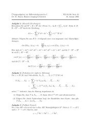
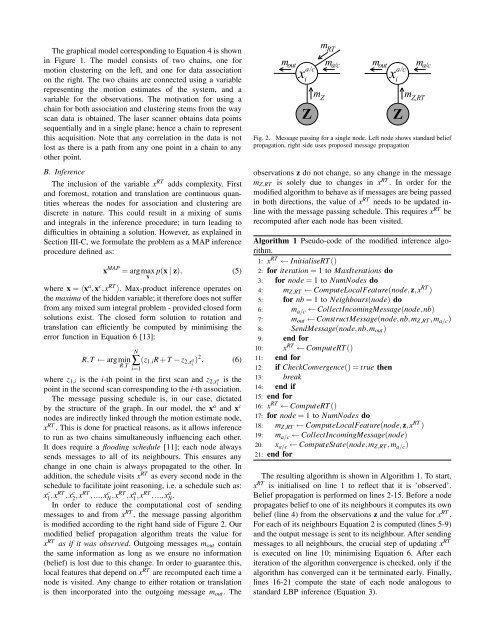
The graphical model corresponding to Equation 4 is shownin Figure 1. The model consists of two chains, one formotion clustering on the left, and one for data associationon the right. The two chains are connected using a variablerepresenting the motion estimates of the system, and avariable for the observations. The motivation for using achain for both association and clustering stems from the wayscan data is obtained. The laser scanner obtains data pointssequentially and in a single plane; hence a chain to representthis acquisition. Note that any correlation in the data is notlost as there is a path from any one point in a chain to anyother point.B. InferenceThe inclusion of the variable x RT adds complexity. Firstand foremost, rotation and translation are continuous quantitieswhereas the nodes for association and clustering arediscrete in nature. This could result in a mixing of sumsand integrals in the inference procedure; in turn leading todifficulties in obtaining a solution. However, as explained inSection III-C, we formulate the problem as a MAP inferenceprocedure defined as:x MAP = argmax p(x | z), (5)xwhere x = 〈x a ,x c ,x RT 〉. Max-product inference operates onthe maxima of the hidden variable; it therefore does not sufferfrom any mixed sum integral problem - provided closed formsolutions exist. The closed form solution to rotation andtranslation can efficiently be computed by minimising theerror function in Equation 6 [13]:R,T ← argminR,TN∑i=1(z 1,i R+T − z 2,x ai) 2 , (6)where z 1,i is the i-th point in the first scan and z 2,x aiis thepoint in the second scan corresponding to the i-th association.The message passing schedule is, in our case, dictatedby the structure of the graph. In our model, the x a and x cnodes are indirectly linked through the motion estimate node,x RT . This is done for practical reasons, as it allows inferenceto run as two chains simultaneously influencing each other.It does require a flooding schedule [11]; each node alwayssends messages to all of its neighbours. This ensures anychange in one chain is always propagated to the other. Inaddition, the schedule visits x RT as every second node in theschedule to facilitate joint reasoning, i.e. a schedule such as:x1 c,xRT ,x2 c,xRT ,...,xN c ,xRT ,x1 a,xRT ,...,xN a .In order to reduce the computational cost of sendingmessages to and from x RT , the message passing algorithmis modified according to the right hand side of Figure 2. Ourmodified belief propagation algorithm treats the value forx RT as if it was observed. Outgoing messages m out containthe same information as long as we ensure no information(belief) is lost due to this change. In order to guarantee this,local features that depend on x RT are recomputed each time anode is visited. Any change to either rotation or translationis then incorporated into the outgoing message m out . Themouta/cx iZmmZRTma/cmouta/cx iZmmZ,RTFig. 2. Message passing for a single node. Left node shows standard beliefpropagation, right side uses proposed message propagationobservations z do not change, so any change in the messagem Z,RT is solely due to changes in x RT . In order for themodified algorithm to behave as if messages are being passedin both directions, the value of x RT needs to be updated inlinewith the message passing schedule. This requires x RT berecomputed after each node has been visited.Algorithm 1 Pseudo-code of the modified inference algorithm.1: x RT ← InitialiseRT()2: for iteration = 1 to MaxIterations do3: for node = 1 to NumNodes do4: m Z,RT ← ComputeLocalFeature(node,z,x RT )5: for nb = 1 to Neighbours(node) do6: m a/c ← CollectIncomingMessage(node,nb)7: m out ← ConstructMessage(node,nb,m Z,RT ,m a/c )8: SendMessage(node,nb,m out )9: end for10: x RT ← ComputeRT()11: end for12: if CheckConvergence() = true then13: break14: end if15: end for16: x RT ← ComputeRT()17: for node = 1 to NumNodes do18: m Z,RT ← ComputeLocalFeature(node,z,x RT )19: m a/c ← CollectIncomingMessage(node)20: x a/c ← ComputeState(node,m Z,RT ,m a/c )21: end forThe resulting algorithm is shown in Algorithm 1. To start,x RT is initialised on line 1 to reflect that it is ’observed’.Belief propagation is performed on lines 2-15. Before a nodepropagates belief to one of its neighbours it computes its ownbelief (line 4) from the observations z and the value for x RT .For each of its neighbours Equation 2 is computed (lines 5-9)and the output message is sent to its neighbour. After sendingmessages to all neighbours, the crucial step of updating x RTis executed on line 10; minimising Equation 6. After eachiteration of the algorithm convergence is checked, only if thealgorithm has converged can it be terminated early. Finally,lines 16-21 compute the state of each node analogous tostandard LBP inference (Equation 3).a/c
C. Feature DescriptionCRFs owe much of their popularity to the feature functionsf c in Equation 1. These encapsulate domain specific knowledgewhich can subsequently be used in the probabilisticframework of the CRF. For completeness a brief descriptionof each feature is provided below. The reader is referred to[19], [23] for more detailed descriptions.1) Association Local Features: A first class of associationlocal features use geometric properties of the data to identifypatterns (shapes) around a single point, say point i, in thefirst scan. They then try to find the same pattern around eachpoint in the second scan. The resulting difference is an errormetric; points in the second scan that have a similar pattern(a small value for the error metric) are more likely candidatesfor association to point i in the first scan. The pattern findingfeatures are:• Distance: Uses the distance to its first, third or fifthneighbour.• Angular: Uses the angle between the first, third or fifthneighbours on either side.• Geodesic: Uses the accumulated distance to its first,third or fifth neighbour; visiting all points in between.• Radius: Uses the range value.In addition to the shape based features above, two otherfeatures are used. These use the structure of the data andoptionally contextual information.• Translation: Uses the distance between a point in thefirst scan with every point in the second scan - analogousto ICP.• Registered Translation: Transforms each point in thefirst scan according to its motion estimate. Then usesthe distance between the transformed point and everypoint in the second scan.The above features are not directly used in Equation 1.They are, instead, used as inputs to boosting [7], [19]. Theoutputs of boosting (the experiments employ AdaBoost [6]with 50 decision stumps) are used as local feature valuesin Equation 1. Using boosting results in better estimates forthe local potentials. There are two boosting features used forassociation: 1) Data Boosting computes the likely associationsand 2) Outlier Boosting determines the likelihood thata point is an outlier.2) Association Pairwise Features: These features fallroughly into two categories. Those that use the structure ofthe scan acquisition and those that use the observations.The first category of features are those that use scanacquisition structure. In an ideal world, without noisy measurementsand outliers, it would be straight forward to relatethe association of node i with that of node i + 1. If nodei associates to point j then node i + 1 can reasonably beexpected to associate to point j+ 1.• Sequence: Expresses the sequential nature of associationby an identity matrix with the diagonal shifted.• Pairwise Outlier: Expresses how outliers impact onassociation transitions - from inlier to outlier and viceversa.The second category of pairwise features operate similarlyto the pattern finding local features. They use a measurebetween two points on an edge in the first scan and comparethis measure with all possible combinations of this measurein the second scan. The comparison produces a metric ofhow pairs of points are related between the two scans (i.e. atransition).• Pairwise Distance: Uses the distance between points oneither end of an edge.• Pairwise Translation: Uses the vector between twopoints corresponding to an edge.3) Clustering Local Features: The purpose of these featuresis to determine whether points are part of the staticbackground, part of a dynamic object or are outliers.• Cluster Distance: Uses distance between two scans tocluster points based on their motion.• Outlier: Uses a threshold value to indicate if the pointis an outlier.• Cluster Inlier Enforces inlier consistency between associationand clustering.4) Clustering Pairwise Features: With the exception ofthe outlier feature, all these features cluster by incorporatingneighbourhood information.• Sequence: Enforces if neighbouring points belong to thesame cluster; an identity matrix.• Neighbour Weight: Captures (non-)neighbouring relationships;scaled by the distance between the points.• Neighbour Stiffness: Captures (non-)neighbouring relationships;scaled by the distance between associatedpairs of neighbouring points.• Neighbour Distance: Expresses that points belonging tothe same cluster should preserve their relative distanceafter transformation.• Pairwise Outlier: Expresses how outliers impact oncluster transitions - from inlier to outlier and vice versa.V. EXPERIMENTSWe perform experiments using data collected with a laserscanner mounted on a car travelling around the University ofSydney campus [23]. 31 pairs of scans containing both staticand dynamic objects were manually annotated. The 31 scanpairs can be divided into 8 subsets; each subset consistingof sequential scan pairs. A single scan contains on averageabout 300 points. As a result the proposed model consists ofa graph of 600 nodes (300 association + 300 clustering). Theclustering nodes are initialised with 5 states for each nodewhile the association nodes will have on average 301 states.The proposed joint model is compared to three techniquesthat compute laser point association and motion clusteringas separate tasks. The first technique employs ICP and theoutput associations provide translation and rotation parametersfrom K-Means clustering [15]. The second techniqueuses CRF-Matching [19] instead of ICP for association andagain K-Means for clustering. Note that K-Means requiresthe number of clusters to be defined in advance. In theexperiments the number of clusters is set to 4 - the maximum
Page 1 and 2: An Integrated Probabilistic Model f
Page 3: Construction of the messages is per
Page 7 and 8: KMeans (ICP) ResultsKMeans (CRF−M

An Integrated Probabilistic Model for Scan-Matching, Moving Object ...

Create successful ePaper yourself

Delete template?

Save as template?