An Integrated Probabilistic Model for Scan-Matching, Moving Object ...

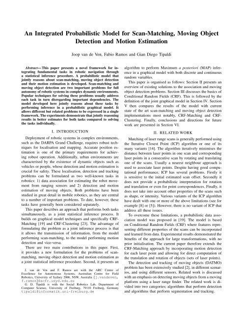
An Integrated Probabilistic Model for Scan-Matching, Moving ObjectDetection and Motion EstimationJoop van de Ven, Fabio Ramos and Gian Diego TipaldiAbstract— This paper presents a novel framework for integratingfundamental tasks in robotic navigation througha statistical inference procedure. A probabilistic model thatjointly reasons about scan-matching, moving object detectionand their motion estimation is developed. Scan-matching andmoving object detection are two important problems for fullautonomy of robotic systems in complex dynamic environments.Popular techniques for solving these problems usually addresseach task in turn disregarding important dependencies. Themodel developed here jointly reasons about these tasks byperforming inference in a probabilistic graphical model. Itallows different but related problems to be expressed in a singleframework. The experiments demonstrate that jointly reasoningresults in better estimates for both tasks compared to solvingthe tasks individually.I. INTRODUCTIONDeployment of robotic systems in complex environments,such as the DARPA Grand Challenge, requires robust techniquesfor localisation and mapping. Accurate position estimationis one of the primary requirements for achievingrobust operation. Additionally, urban environments arecharacterised by the existence of dynamic objects such asvehicles or people, whose detection and motion estimation iscrucial for safety. These localisation, detection and trackingproblems can be formulated as two well-known tasks inrobotics: 1) data association for estimating the robot movementfrom ranging sensors and 2) detection and motionestimation of moving objects. Both problems have beenstudied in great detail in mobile robotics, as they are centralto a number of important problems. To date, however, thesetasks have generally been considered separately.This paper describes an approach that performs both taskssimultaneously, as a joint statistical inference process. Itbuilds on graphical model techniques and specifically CRF-Matching [19] and CRF-Clustering [23]. The advantage offormulating the problem as a joint inference process is thatit allows the transmission of information, from the modelperforming scan-matching, to the model performing motiondetection and vice-versa.There are two main contributions in this paper. First,it provides a new formulation for the problems of scanmatching,moving object detection and motion estimation asa joint statistical inference procedure. Second, it presents anJ. van de Ven and F. Ramos are with the ARC Centre ofExcellence for Autonomous Systems, Australian Centre for FieldRobotics, University of Sydney 2006, NSW, Australia {j.vandeven,f.ramos}@acfr.usyd.edu.auG. D. Tipaldi is with the Social Robotics Lab, Department ofComputer Science, University of Freiburg, 79110 Freiburg, Germanytipaldi@informatik.uni-freiburg.dealgorithm to perform Maximum a posteriori (MAP) inferencein a graphical model with both discrete and continuousrandom variables.This paper is organised as follows: Section II presents anoverview of existing solutions to the association and movingobject detection problems. Section III discusses the basics ofConditional Random Fields (CRF). This is followed by thedefinition of the joint graphical model in Section IV. SectionV then compares the results of the model with currentstate of the art scan-matching and moving object detectionimplementations most notably, CRF-Matching and CRF-Clustering. Finally, conclusions and directions for futurework are presented in Section VI.II. RELATED WORKMatching of laser range scans is generally performed usingthe Iterative Closest Point (ICP) algorithm or one of itsmany variants [14]. The algorithm iteratively minimises thedistance between laser points in one scan and correspondinglaser points in a consecutive scan by rotating and translatingone of the scans. Usually a nearest neighbour approach isused to associate laser points. Despite having good computationalperformance, ICP has several problems. Firstly itis sensitive to the initial estimated scan offset. Secondly itdoes not provide a probabilistic interpretation for rotationand translation or even for point correspondences. Finally, itdoes not take into account other properties of the scans suchas shape, or intensity. Various variants of the ICP algorithmhave dealt with one or more of the above limitations (see forexample [8] or [5]). However, there is no variant of ICP thataddress all these issues.To overcome these limitations, a probabilistic data associationmodel was proposed in [19]. The model is basedon Conditional Random Fields (CRF) where features representingdifferent properties of the scans can be incorporatedand learned from data. Experimental results demonstrated thebenefits of the approach for large transformations, with noprior initialisation. The current paper therefore extends theCRF-Matching approach by incorporating motion detectionfor each laser point and allowing for direct computation ofthe translation and rotation of objects (sets of laser points).The detection and tracking of moving objects (DATMO)problem has been extensively studied [2], in different scenarios,and using different sensors. Related work is discussedwith an emphasis on detecting moving objects from a movingplatform using a laser range finder. The related work is dividedinto two categories; algorithms that perform detectionand algorithms that perform segmentation and tracking.

The detection algorithms address the problem in terms ofseparating the data into static and dynamic clusters. Dynamicpoints are used for tracking of dynamic objects while thestatic points are used to obtain better motion estimates forthe moving platform.Hähnel et al. [9] detect moving points in range datausing an Expectation-Maximisation (EM) based approach.The algorithm maximises the likelihood of the data using ahidden variable expressing the nature of the points (static ordynamic).In [26], two separate maps are maintained; one for thestatic part of the environment and one for the dynamic. Themaps employ a modified occupancy grid framework whichalso infers if points are static or dynamic.Rodriguez-Losada and Minguez [20] improve data associationfor the ICP algorithm. They introduce a new metricwhich models dynamic objects to better reflect the realmotion of the robot. Their approach however, does notdistinguish moving objects from outliers.The second category of algorithms focuses on objectsegmentation and tracking. Anguelov et al. [1], [4] detectmoving points using simple differencing and then apply amodified EM algorithm for clustering the different objects.In [25] an integrated solution to the mapping and trackingproblem is defined: static points are used for mappingand dynamic points for tracking. Data differencing andconsistency-based motion detection [24] is used for thedetection and segmentation of dynamic points. Points areclassified as static or dynamic and clustered into segments;when a segment contains enough dynamic points is considereddynamic. Montesano et al. [16] subsequently improvethe classification procedure of [25] by jointly solving it in asequential manner.Schulz et al. [22] use a feature based approach to detectmoving objects; the features used are the local minima ofthe laser data. The objects are then tracked using a jointprobabilistic data association filter (JPDAF).The focus for most of these approaches is on trackingdifferent objects under different hypothesis. The detectionpart, however, is mainly based on heuristics such as scan differencing.The detection routines observe the actual positionof the object and the velocities are computed by the trackingalgorithm. CRF-Clustering [23] on the other hand, appliesa feature based graphical model to the data. This allows itto reason about the underlying motion of points; it detectsand tracks the objects in a single framework, iterativelyimproving the estimates.The work presented in [10] allows different, state-ofthe-artalgorithms, to be combined in a cascaded/sequentialframework. The approach treats each algorithm as a ”blackbox”though it allows limited unidirectional interactionthrough feature vectors. The model proposed in this paperon the other hand, integrates and extends the CRF-Clusteringand CRF-Matching approaches into a single framework.Motion estimates are computed in-line with motion detectionand data association, allowing for joint reasoning enhancedestimates.III. PRELIMINARIESA. Conditional Random FieldsConditional Random Fields [12] (CRFs) are undirectedgraphical models that represent probability distributions; thevertices of the graph index random variables while the edgesof the graph capture relationships between variables. In thecase of CRFs the distribution is conditional (a probabilisticdiscriminative model); the hidden variables x = 〈x 1 ,x 2 ,...,x n 〉are globally conditioned on the observations z; p(x | z).Let C be the set of all cliques of the graph. The distributionmust then factorise as a product of clique potentialsφ c (x c ,z), where c ∈ C and x c are the hidden variables ofthe clique. Clique potentials are commonly expressed bya log-linear combination of feature functions, φ c (x c ,z) =exp ( w T c · f c (x c ,z) ) , resulting in the definition of a CRF as:(p(x | z) = 1Z(z) exp ∑ w T c · f c (x c ,z)c∈C). (1)Here Z(z) = ∑ x exp(∑ c∈C w T c · f c (x c ,z)) is the partitionfunction; it normalises the exponential ensuring Equation 1is a proper distribution. C is again the set of all cliquesin the graph. w c are parameters (or weights). The featurefunctions f c extract feature vectors given the value of theclique variables x c and observations z.B. Parameter LearningThe weights w c express the relative importance of eachfeature function. As such they play an important role indetermining the shape of the distribution. The weights arelearnt by maximising the conditional likelihood (Equation1) given labelled training data. In our case, this is computationallyintractable as the partition function Z(z) sums overthe entire state space of all hidden variables. A typical graphin the experiments contains on average 600 hidden variableswith an approximate total number of states of 100000.We therefore use maximum pseudo-likelihood learning[3]. Maximum pseudo-likelihood learning approximates thejoint by considering, for each hidden variable, only itsneighbours in the graph: the Markov blanket. As a result,the partition function is approximated by summing over thestate space of individual hidden variables.C. InferenceThe model defined in the next section is a joint distributionover data association, motion detection and motion clusteringhidden variables. The desired outcome of inference is aconfiguration of the hidden variables for which the jointdistribution achieves its maximum; a maximum a posteriori(MAP) inference problem. The proposed algorithm is avariation on Max-Product Loopy Belief Propagation.Belief Propagation (BP) [18] is a class of inferencealgorithms in which each node sends messages to each ofits neighbours in the graph. The messages convey what anode believes its neighbours’ state should be given its ownstate. The received messages together with a node’s ownbelief are then used to compute the MAP configuration.

Construction of the messages is performed using the Max-Product algorithm [18] as follows:)m i j (x i ) = max(φ(x j ,z)φ(x i ,x j ,z)x j∏ m k j (x j ) , (2)k∈N ( j)\iwhere m i j (x i ) is the message node j sends to node i.φ(x j ,z) is the local clique potential for node j. Local cliquepotentials represent what a node believes its state is, giventhe observations. Computation of the local potential can bevisualised as passing a message from the observation to thenode, see m Z in the left hand side of Figure 2. φ(x i ,x j ,z) isthe pairwise clique potential. Pairwise potentials relate nodesi and j on either end of an edge. They transform the belief ofnode j into a form suitable for node i and vice versa. Lastlya product of all incoming messages is computed, except fromthe node to which the message is being sent. In the left handside of Figure 2, the incoming messages are represented bym a/c and m RT , while the outgoing messages m i j is visualisedas m out .BP generates exact solution for graphs such as treesor polytrees. The proposed model is neither a tree nor apolytree. We therefore use Loopy Belief Propagation (LBP)[17], an approximation to BP. In LBP, message propagationcontinuous until the difference in messages falls below somethreshold, or until a maximum number of iterations has beenreached. Once message propagation is finished, the maximalconfiguration can be found by applying Equation 3 to eachnode in turn,)xi ∗ ∈ argmax(φ(x i ,z)x i∏ m ji (x i ) . (3)j∈N (i)Here x i indicates the node while xi∗ is its maximal configuration.As can be seen, maximisation is performed ona node’s own belief (local potential) combined with allincoming messages. The maximal configuration for the nodeis then simply a state for which the combined belief ismaximal.IV. JOINT MODEL FOR SCAN MATCHING ANDCLUSTERINGA. Model DefinitionAs discussed in Section II, solutions for motion detection/estimationand scan matching are generally defined independently.In reality though, both scan matching and movingobject detection are strongly interdependent; laser pointsbelonging to the same object will have similar associationsand vice versa.Following [23], motion detection is formulated as a clusteringproblem. The environment consists of one or more dynamicobjects (one cluster for each dynamic object) togetherwith a cluster representing the background. Laser points areclustered based on the object they belong to (i.e. those withsimilar motion patterns). Additionally, here we also includean outlier cluster for those points which can not reasonablybe considered part of an object. Given the clusters for staticx c 1x c 2x c Nx RT x a Nx a 2zx a 1Fig. 1. Graphical model for combined scan matching, motion clusteringand motion estimation.and dynamic objects, motion estimation then determines therotation and translation of each object.A model (Equation 4), is proposed to solve moving objectdetection, motion estimation and data association simultaneously.p(x | z) = p(x a ,x c ,x RT | z). (4)Equation 4 expresses a conditional distribution of threesets of hidden variables (x a , x c , x RT ) given an observation z.The observation consists of two laser scans for which associationand motion detection/estimation is to be determined.The variables x a consists of N association nodes, where Nis the number of points in the first scan. Each of these nodesis discrete with M+1 states; M being the number of points inthe second scan. The states of x a at node i have the followinginterpretation: The first state indicates the likelihood thatpoint i in the first scan associates to point 1 in the secondscan. The second state is the likelihood of association to thesecond point in the second scan, etc. Finally, the M+1 staterepresents the likelihood that point i is an outlier.The variables x c consists of N motion detection nodes,with D discrete states each. Here D represents the numberof clusters a point can belong to. The interpretation isanalogous to that of association. The first state represents thelikelihood that point i belongs to the first object (cluster),etc. By convention, the last state D represents the clusterfor outliers. The choice on number of clusters D may beguided using a priori knowledge. If no such knowledge isavailable then D can be set to M+1, i.e. start with a clusterfor each point. Once the inference algorithm has clusteredthe points, any vacuous clusters can safely be discarded. Theinference algorithm will assign probability mass to each nodeaccording to the likelihood of belonging to a cluster. Clustersthat have no significant probability mass for all nodes aretherefore not likely, and can be removed. For computationalreasons it is advisable to reduce the number of clusters.Lastly, the variable x RT represents the rotational R andtranslational T parameters of each object in the systemexcept the outlier cluster. As such this is a multi-dimensionalcontinuous variable. Note that the robot motion can beobtained from the rotation and translation parameters of thebackground object.

The graphical model corresponding to Equation 4 is shownin Figure 1. The model consists of two chains, one formotion clustering on the left, and one for data associationon the right. The two chains are connected using a variablerepresenting the motion estimates of the system, and avariable for the observations. The motivation for using achain for both association and clustering stems from the wayscan data is obtained. The laser scanner obtains data pointssequentially and in a single plane; hence a chain to representthis acquisition. Note that any correlation in the data is notlost as there is a path from any one point in a chain to anyother point.B. InferenceThe inclusion of the variable x RT adds complexity. Firstand foremost, rotation and translation are continuous quantitieswhereas the nodes for association and clustering arediscrete in nature. This could result in a mixing of sumsand integrals in the inference procedure; in turn leading todifficulties in obtaining a solution. However, as explained inSection III-C, we formulate the problem as a MAP inferenceprocedure defined as:x MAP = argmax p(x | z), (5)xwhere x = 〈x a ,x c ,x RT 〉. Max-product inference operates onthe maxima of the hidden variable; it therefore does not sufferfrom any mixed sum integral problem - provided closed formsolutions exist. The closed form solution to rotation andtranslation can efficiently be computed by minimising theerror function in Equation 6 [13]:R,T ← argminR,TN∑i=1(z 1,i R+T − z 2,x ai) 2 , (6)where z 1,i is the i-th point in the first scan and z 2,x aiis thepoint in the second scan corresponding to the i-th association.The message passing schedule is, in our case, dictatedby the structure of the graph. In our model, the x a and x cnodes are indirectly linked through the motion estimate node,x RT . This is done for practical reasons, as it allows inferenceto run as two chains simultaneously influencing each other.It does require a flooding schedule [11]; each node alwayssends messages to all of its neighbours. This ensures anychange in one chain is always propagated to the other. Inaddition, the schedule visits x RT as every second node in theschedule to facilitate joint reasoning, i.e. a schedule such as:x1 c,xRT ,x2 c,xRT ,...,xN c ,xRT ,x1 a,xRT ,...,xN a .In order to reduce the computational cost of sendingmessages to and from x RT , the message passing algorithmis modified according to the right hand side of Figure 2. Ourmodified belief propagation algorithm treats the value forx RT as if it was observed. Outgoing messages m out containthe same information as long as we ensure no information(belief) is lost due to this change. In order to guarantee this,local features that depend on x RT are recomputed each time anode is visited. Any change to either rotation or translationis then incorporated into the outgoing message m out . Themouta/cx iZmmZRTma/cmouta/cx iZmmZ,RTFig. 2. Message passing for a single node. Left node shows standard beliefpropagation, right side uses proposed message propagationobservations z do not change, so any change in the messagem Z,RT is solely due to changes in x RT . In order for themodified algorithm to behave as if messages are being passedin both directions, the value of x RT needs to be updated inlinewith the message passing schedule. This requires x RT berecomputed after each node has been visited.Algorithm 1 Pseudo-code of the modified inference algorithm.1: x RT ← InitialiseRT()2: for iteration = 1 to MaxIterations do3: for node = 1 to NumNodes do4: m Z,RT ← ComputeLocalFeature(node,z,x RT )5: for nb = 1 to Neighbours(node) do6: m a/c ← CollectIncomingMessage(node,nb)7: m out ← ConstructMessage(node,nb,m Z,RT ,m a/c )8: SendMessage(node,nb,m out )9: end for10: x RT ← ComputeRT()11: end for12: if CheckConvergence() = true then13: break14: end if15: end for16: x RT ← ComputeRT()17: for node = 1 to NumNodes do18: m Z,RT ← ComputeLocalFeature(node,z,x RT )19: m a/c ← CollectIncomingMessage(node)20: x a/c ← ComputeState(node,m Z,RT ,m a/c )21: end forThe resulting algorithm is shown in Algorithm 1. To start,x RT is initialised on line 1 to reflect that it is ’observed’.Belief propagation is performed on lines 2-15. Before a nodepropagates belief to one of its neighbours it computes its ownbelief (line 4) from the observations z and the value for x RT .For each of its neighbours Equation 2 is computed (lines 5-9)and the output message is sent to its neighbour. After sendingmessages to all neighbours, the crucial step of updating x RTis executed on line 10; minimising Equation 6. After eachiteration of the algorithm convergence is checked, only if thealgorithm has converged can it be terminated early. Finally,lines 16-21 compute the state of each node analogous tostandard LBP inference (Equation 3).a/c

C. Feature DescriptionCRFs owe much of their popularity to the feature functionsf c in Equation 1. These encapsulate domain specific knowledgewhich can subsequently be used in the probabilisticframework of the CRF. For completeness a brief descriptionof each feature is provided below. The reader is referred to[19], [23] for more detailed descriptions.1) Association Local Features: A first class of associationlocal features use geometric properties of the data to identifypatterns (shapes) around a single point, say point i, in thefirst scan. They then try to find the same pattern around eachpoint in the second scan. The resulting difference is an errormetric; points in the second scan that have a similar pattern(a small value for the error metric) are more likely candidatesfor association to point i in the first scan. The pattern findingfeatures are:• Distance: Uses the distance to its first, third or fifthneighbour.• Angular: Uses the angle between the first, third or fifthneighbours on either side.• Geodesic: Uses the accumulated distance to its first,third or fifth neighbour; visiting all points in between.• Radius: Uses the range value.In addition to the shape based features above, two otherfeatures are used. These use the structure of the data andoptionally contextual information.• Translation: Uses the distance between a point in thefirst scan with every point in the second scan - analogousto ICP.• Registered Translation: Transforms each point in thefirst scan according to its motion estimate. Then usesthe distance between the transformed point and everypoint in the second scan.The above features are not directly used in Equation 1.They are, instead, used as inputs to boosting [7], [19]. Theoutputs of boosting (the experiments employ AdaBoost [6]with 50 decision stumps) are used as local feature valuesin Equation 1. Using boosting results in better estimates forthe local potentials. There are two boosting features used forassociation: 1) Data Boosting computes the likely associationsand 2) Outlier Boosting determines the likelihood thata point is an outlier.2) Association Pairwise Features: These features fallroughly into two categories. Those that use the structure ofthe scan acquisition and those that use the observations.The first category of features are those that use scanacquisition structure. In an ideal world, without noisy measurementsand outliers, it would be straight forward to relatethe association of node i with that of node i + 1. If nodei associates to point j then node i + 1 can reasonably beexpected to associate to point j+ 1.• Sequence: Expresses the sequential nature of associationby an identity matrix with the diagonal shifted.• Pairwise Outlier: Expresses how outliers impact onassociation transitions - from inlier to outlier and viceversa.The second category of pairwise features operate similarlyto the pattern finding local features. They use a measurebetween two points on an edge in the first scan and comparethis measure with all possible combinations of this measurein the second scan. The comparison produces a metric ofhow pairs of points are related between the two scans (i.e. atransition).• Pairwise Distance: Uses the distance between points oneither end of an edge.• Pairwise Translation: Uses the vector between twopoints corresponding to an edge.3) Clustering Local Features: The purpose of these featuresis to determine whether points are part of the staticbackground, part of a dynamic object or are outliers.• Cluster Distance: Uses distance between two scans tocluster points based on their motion.• Outlier: Uses a threshold value to indicate if the pointis an outlier.• Cluster Inlier Enforces inlier consistency between associationand clustering.4) Clustering Pairwise Features: With the exception ofthe outlier feature, all these features cluster by incorporatingneighbourhood information.• Sequence: Enforces if neighbouring points belong to thesame cluster; an identity matrix.• Neighbour Weight: Captures (non-)neighbouring relationships;scaled by the distance between the points.• Neighbour Stiffness: Captures (non-)neighbouring relationships;scaled by the distance between associatedpairs of neighbouring points.• Neighbour Distance: Expresses that points belonging tothe same cluster should preserve their relative distanceafter transformation.• Pairwise Outlier: Expresses how outliers impact oncluster transitions - from inlier to outlier and vice versa.V. EXPERIMENTSWe perform experiments using data collected with a laserscanner mounted on a car travelling around the University ofSydney campus [23]. 31 pairs of scans containing both staticand dynamic objects were manually annotated. The 31 scanpairs can be divided into 8 subsets; each subset consistingof sequential scan pairs. A single scan contains on averageabout 300 points. As a result the proposed model consists ofa graph of 600 nodes (300 association + 300 clustering). Theclustering nodes are initialised with 5 states for each nodewhile the association nodes will have on average 301 states.The proposed joint model is compared to three techniquesthat compute laser point association and motion clusteringas separate tasks. The first technique employs ICP and theoutput associations provide translation and rotation parametersfrom K-Means clustering [15]. The second techniqueuses CRF-Matching [19] instead of ICP for association andagain K-Means for clustering. Note that K-Means requiresthe number of clusters to be defined in advance. In theexperiments the number of clusters is set to 4 - the maximum

Fig. 3. A sequence of 4 scan association results with magnified dynamic object associations. Top row, left to right: ICP, CRF-Matching. Bottom row,left to right: Proposed Joint Model, Ground Truth. Lines indicate MAP associations between laser points (outlier points have no connecting lines). Alltechniques perform well on the background. Looking at the dynamic object, ICP is unable to associate the dynamic object. CRF-Matching does reasonablywell but struggles in the encircled area. The proposed model correctly associates points in the direction of motion.Technique Accuracy(%) SED Outlier(%) (true/ratio)ICP 69.19 119.10 34.60 (11.07/89.79)CRF-Matching 71.03 116.16 13.01 (11.07/57.93)Combined Model 74.13 96.13 12.96 (11.07/73.37)TABLE IASSOCIATION METRICS FOR THE DIFFERENT TECHNIQUES.based on the ground truth. Finally, the third technique usesCRF-Matching and CRF-Clustering in turn. CRF-Clusteringis essentially the clustering layer in Figure 1 while CRF-Matching is the association layer. This technique equates toremoving all the links connecting the two chains through x RTin Figure 1 - this allows for a clear comparison and showsthe advantage of joint reasoning about motion detection andscan matching.Experiments are conducted in a leave-one-out cross validationfashion. All CRF based techniques require learningof the weights (18/12/30 weights for CRF-Matching/CRF-Clustering/proposed model respectively). As such, 30 scanpairs are used to training the model and 1 scan pair is usedfor testing. This process is then repeated for each of the 31scan pairs and averaging the results. This scheme ensures thatthe results represent the model’s ability to deal with each ofthe scan pairs individually. ICP and K-Means do not requiretraining, for these techniques the average over the 31 scansis computed for fair comparison.Figure 3 shows examples of association results for eachof the different association techniques together with theassociation result of the proposed model and ground truth.The figures contain 4 sequential scans, with the blue scanbeing the most recently acquired scan. The dynamic objectis magnified in all figures. Looking at the results it is clearthat all perform quite well on the static points. The differenceis how the different techniques deal with the dynamic object.ICP does poorly, this is to be expected since ICP uses onlynearest neighbour information for determining associations.CRF-Matching does significantly better due to the fact thatit performs associations based on local shape information. Itis, however, unable to correctly associate the points in thelower section (circled) of the dynamic object as the localshape of these points is similar. The proposed model on theother hand has clustering information available. This allowsit to correctly associate in the direction of motion.The output of motion detection is analogous. Figure 4shows the results for a single scan pair - for clarity. Ascan be seen, the results for K-Means clustering dependvery much on the quality of the associations. Using ICPfor the associations, the results are inconsistent. K-Meanswith CRF-Matching does significantly better but is adverselyaffected by K-Means requiring the number of clusters to bedetermined in advance. CRF-Clustering does better, becauselike CRF-Matching, CRF-Clustering is able to infer morefrom the scans. The proposed model does exceptionally well.It correctly determines the number of clusters in the dataand there are very few mis-classifications - only a few in thecorner of the dynamic object.In addition to the visual comparison, a quantitative measureof similarity between the association/clustering resultsand the ground-truth is given. Tables I and II present aperformance comparison in terms of accuracy, String EditDistance (SED) [21] and outlier detection. The accuracy is

KMeans (ICP) ResultsKMeans (CRF−Matching) ResultsCRF−Clustering Results151515101010y−coordinate (m)50y−coordinate (m)50y−coordinate (m)50−5−5−5−100 2 4 6 8 10 12 14 16x−coordinate (m)Combined Model Results−100 2 4 6 8 10 12 14 16x−coordinate (m)Ground Truth Results−100 2 4 6 8 10 12 14 16x−coordinate (m)15151010y−coordinate (m)50y−coordinate (m)50−5−5−100 2 4 6 8 10 12 14 16x−coordinate (m)−100 2 4 6 8 10 12 14 16x−coordinate (m)Fig. 4. Motion detection results. Top row, left to right; K-Means initialised with ICP, K-Means initialised with CRF-Matching, CRF-Clustering. Bottomrow, left to right: Proposed Joint Model, Ground Truth. Different colours indicate different clusters (dark green for the static background), outlier pointshave no coloured circle. K-Means (ICP) has very poor results mainly due the poor associations. CRF-Clustering and K-Means (CRF-Matching) have similarresults, though CRF-Clustering results are a little more consistent. The proposed model has near perfect result.Technique Accuracy(%) SED Outlier(%) (true/ratio)K-Means (ICP) 43.16 243.87 34.60 (11.07/89.79)K-Means (CRF) 60.42 215.55 13.01 (11.07/57.93)CRF-Clustering 60.04 190.03 24.35 (11.07/55.64)Combined Model 83.22 79.61 13.12 (11.07/73.37)TABLE IIMOTION DETECTION METRICS FOR THE TECHNIQUES.Technique Rotation Error (radians) Translation Error (m)K-Means (ICP) 0.02 1.01K-Means (CRF) 0.04 0.77CRF-Clustering 0.05 0.88Combined Model 0.03 0.56TABLE IIIMOTION ESTIMATION METRICS FOR THE TECHNIQUES.the percentage of correctly associated/clustered points 1 . TheSED is a measure of how many permutations are requiredon a string to make it match another. Here the two stringsare the association/clustering results on the one hand and theground-truth on the other. Therefore, the less the SED thebetter. Finally the percentage of outliers gives a measure ofhow useful the solution is. Solutions with a high percentageof outliers may give a reasonable accuracy/SED but theyare not practical. Outliers are presented as the percentage ofoutliers found, together with the true percentage of outliers(from the ground-truth), and a ratio (percentage) of groundtruthoutliers that were found.Table I confirms the visual results of Figure 3 for the completedata set. The combined model outperforms both ICPand CRF-Matching. A note on the results of ICP. Based onthe metrics provided, accuracy & SED, one might be inclinedto conclude that ICP did rather well. To a certain extent this1 A good association accuracy metric is difficult to define; associationsnear to the true associations require a different penalty from those furtheraway.is true; the different scans were reasonably closely alignedand there are relatively few dynamic points (ratio of dynamicover static points is ∼ 0.14). ICP’s solution however, consists(on average) of more than a third outliers. It should havefound around 11 percent of outliers. This high percentageof outliers subsequently results in poor estimates for motiondetection. Metric comparison for the motion parameters isgiven in Tables II and III. The comparison shows againthat joint reasoning about association and motion producesbetter results. Table III shows average results for correctlyclustered objects only. The relatively good performance ofthe K-Means based techniques is primarily due to correctclustering of the background.VI. CONCLUSIONS AND FUTURE WORKSThis paper presented a probabilistic model that jointlyreasons about laser point association, motion clustering andmotion estimation. The experimental results have demonstratedthat much can be gained by modelling different (butdependent) problems in the same statistical framework. We

elieve the methods presented here are an initial step towardsintegrating multiple tasks in mobile robotics.In its present form, the clustering and association chainmodels are (indirectly) linked using the rotation and translationnode. In future these two models will be directlyconnected thus forming a clustering and association lattice.The lattice more closely represents the dependencies betweenthe two models. The drawback of this is an increment inthe computational complexity. Note that a different graphstructure also allows for different message passing scheduleswith different performance characteristics (see comment onperformance next).Inference in the combined model is slow. For laser scanswith 361 points, this can take up to 4 minutes in our Matlabimplementation - depending on convergence. Analysis hasshown 3 performance bottlenecks. First, some of the pairwisefeatures are poorly implemented. This is exacerbated bythe second bottleneck; the fact that a flooding schedule isused for message passing. Lastly the cost of computingEquation 6. There are, however, several alternatives to speedup inference. One possibility is to constrain the number ofstates in the association model. For example, a particularlaser point can only be associated to one of its 10 nearestneighbours rather than to all 361 points of the other scan.This would significantly reduce the cost of searching for anassociation. As well as a reduction in the computational costof message propagation - the size of the pairwise featurefunctions will be quadratically reduced. Additionally, weplan to investigate better inference algorithms, especiallyones with strong convergence guarantees. In this case, LinearProgramming (LP) relaxations appear as a potential candidate.ACKNOWLEDGEMENTSThis work has been supported by the Rio Tinto Centrefor Mine Automation and the ARC Centre of Excellenceprogramme, funded by the Australian Research Council(ARC) and the New South Wales State Government.REFERENCES[1] D. Anguelov, R. Biswas, D. Koller, B. Limketkai, S. Sanner, andS. Thrun. Learning hierarchical object maps of non-stationary environmentswith mobile robots. In Proc. of the Conference on Uncertaintyin Artificial Intelligence (UAI), 2002.[2] Y. Bar-Shalom and X.-R. Li. Multitarget-Multisensor Tracking:Principles and Techniques. YBS Publishing, 1995.[3] J. Besag. Statistical analysis of non-lattice data. The Statistician, 24,1975.[4] R. Biswas, B. Limketkai, S. Sanner, and S. Thrun. Towards objectmapping in dynamic environments with mobile robots. In Proc. of theIEEE/RSJ International Conference on Intelligent Robots and Systems(IROS), 2002.[5] M. Bosse and R. Zlot. Continuous 3d scan-matching with a spinning2d laser. In Proc. of the IEEE International Conference on Robotics& Automation (ICRA), 2009.[6] Y. Freund and R.E. Schapire. Experiments with a new boostingalgorithm. In Proc. of the International Conference on MachineLearning (ICML), 1996.[7] S. Friedman, D. Fox, and H. Pasula. Voronoi random fields: Extractingthe topological structure of indoor environments via place labeling. InProc. of the International Joint Conference on Artificial Intelligence(IJCAI), 2007.[8] S. Granger and X. Pennee. Multi-scale EM-ICP: A fast and robustapproach for surface registration, 2002. Internal research report,INRIA.[9] D. Hähnel, R. Triebel, W. Burgard, and S. Thrun. Map buildingwith mobile robots in dynamic environments. In Proc. of the IEEEInternational Conference on Robotics & Automation (ICRA), 2003.[10] G. Heitz, S. Gould, A. Saxena, and D. Koller. Cascaded classificationmodels: Combining models for holistic scene understanding. InAdvances in Neural Information Processing Systems (NIPS 2008),2008.[11] F. Kschischang, B. J. Frey, and H. Loeliger. Factor graphs and thesum-product algorithm. IEEE Transactions on Information Theory,47:498–519, 2001.[12] J. Lafferty, A. McCallum, and F. Pereira. Conditional random fields:Probabilistic models for segmenting and labeling sequence data. InProc. of the International Conference on Machine Learning (ICML),2001.[13] F. Lu and E. Milios. Robot pose estimation in unknown environmentsby matching 2D range scans. In IEEE Computer Vision and PatternRecognition Conference (CVPR), 1994.[14] F. Lu and E. Milios. Robot pose estimation in unknown environmentsby matching 2D range scans. Journal of Intelligent and RoboticSystems, 18, 1997.[15] D. J. C. MacKay. Information Theory, Inference, and LearningAlgorithms. Cambridge University Press, 2003.[16] L. Montesano, J. Minguez, and L. Montano. Modeling the staticand the dynamic parts of the environment to improve sensor-basednavigation. In Proc. of the IEEE International Conference on Robotics& Automation (ICRA), 2005.[17] K. Murphy, Y. Weiss, and M. Jordan. Loopy belief propagation forapproximate inference: An empirical study. In Proc. of the Conferenceon Uncertainty in Artificial Intelligence (UAI), 1999.[18] J. Pearl. Probabilistic Reasoning in Intelligent Systems: Networks ofPlausible Inference. Morgan Kaufmann Publishers, Inc., 1988.[19] F. Ramos, D. Fox, and H. Durrant-Whyte. CRF-matching: Conditionalrandom fields for feature-based scan matching. In Proc. of Robotics:Science and Systems, 2007.[20] D. Rodriguez-Losada and J. Minguez. Improved data associationfor icp-based scan matching in noisy and dynamic environments. InProc. of the IEEE International Conference on Robotics & Automation(ICRA), 2007.[21] D. Sankoff and J. Kruskal, editors. Time Warps, String Edits, andMacromolecules: The Theory and Practice of Sequence Comparison.Addison-Wesley, 1983.[22] D. Schulz, W. Burgard, D. Fox, and A. B Cremers. Tracking multiplemoving targets with a mobile robot using particle filters and statisticaldata association. In Proc. of the IEEE International Conference onRobotics & Automation (ICRA), 2001.[23] G. Tipaldi and F. Ramos. Motion clustering and estimation withconditional random fields. In Proc. of the IEEE/RSJ InternationalConference on Intelligent Robots and Systems (IROS), 2009.[24] C. Wang and C. Thorpe. Simultaneous localization and mappingwith detection and tracking of moving objects. In Proc. of the IEEEInternational Conference on Robotics & Automation (ICRA), 2002.[25] C. Wang, C. Thorpe, M. Hebert, S. Thrun, and H. Durrant-Whyte.Simultaneous localization, mapping and moving object tracking. TheInternational Journal of Robotics Research, 26(6), June 2007.[26] D. Wolf and G. Sukhatme. Mobile robot simultaneous localizationand mapping in dynamic environments. Autonomous Robots, 19:53–65, 2005.