1 General Algebraic and Differential Riccati ... - Bradley Bradley

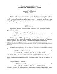
1General Algebraic and DifferentialRiccati Equations from Stochastic LQR ProblemLibin MouDepartment of MathematicsBradley UniversityPeoria, IL 61625Abstract. In this paper we consider a class of matrix Riccati equations arising from stochasticLQR problems. We prove a monotonicity of solutions to the differential Riccati equations, whichleads to a necessary and sufficient condition for the existence of solutions to the algebraic Riccatiequations. In addition, we obtain results on comparison, uniqueness, stabilizability and approximationfor solutions of the algebraic Riccati equations.§ 1. IntroductionThe following differential Riccati equation has been studied in [12] by using the method ofupper and lower solutions.Ú w XXÝ T €E T€TE€G TG€ K € CaTbX X XX " X XÛ aF T€HTG€WbaV€HTHb aF T€HTG€Wbœ!ßÝÜ T a>b œR,"(1)where E is the transpose of E, T œ.>, R is a symmetric matrix, C is a linear map of symmetricmatrices, and EßFßGßHß K ßV and W are bounded and measurable matrix functions with appropriatedimensions. The main results in [12] include an interpretation of upper and lower solutions,comparison theorems, an upper-lower solution theorem, necessary and sufficient conditions forexistence of solutions, an estimation of maximal existence intervals of solutions and an approximationof solutions.X w .T(1):This paper is a continuation ofXXE T€TE€G TG€ K € CaTb[12]. The focus here is the algebraic equation associated withXX X X X XaF T€HTG€WbaV€HTHb aF T€HTG€Wbœ! ,"(2)where EßFßGßHßK ßV and W are constant matrices with appropriate dimensions; see (5) below.The inclusion of the term C is important to stochastic control problems with Markovianjumping noises and differential game problems with state-dependent noises; see [18] and [11], forexample.Equation (2) with C œ! becomesXXE T€TE€G TG€ KXX X X X XaF T€HTG€WbaV€HTHb aF T€HTG€Wbœ! ."(3)Equation (3) arises from the following stochasticlinear quadratic regulator ( LQR) problem of infinite-

3Denote ’ 8 ‘8‚8 XXœ eT­ ÀT œTf, where T is the transpose of T. We write Q " Q#8 8 8( Q" žQ# ) if Q" Q#­ ’ is a positive semidefinite (definite). For a map C À ’ Ä ’ we writeC ! if CaQ b ! for each Q ." " !Assumption. We assume that EßFßGßHßKßVßW and R in equations (1), (2) and (3) are constantmatrices and C À ’ 8 Ä ’8 is a linear map, which satisfy8‚8 8‚5 8XEßG­ ‘ àFßHßW ­ ‘ àV­ ’ 5 ; K, R ­ ’ ; C 0 Þ(5)For a Hilbert space — and an interval M, P_ aMß—b is the space of all bounded and measurable"ß_ _ w _functions from M to —. Furthermore, we define P aMß— b œÖT ­P aMß— bßT ­P aMß — b×ÞThesolution T to (1) is assumed to be in P "ß_ aMß’ 8 b. Since all matrices in (1) are constant, a solution Ton M is actually smooth. The solution T to (2) and (3) is assumed to be in ’ 8 , which may beconsidered as a constant solution to the associated differential equation.As in [12], we abbreviate (1), (2) and (3) asÚ T w € LQaT b€ CaTb œ!ß T a> " b œ Rß (1)Û LQaT b€ CaTbœ!ß(2)Ü LQaTbœ!ß(3)where LQaTb œK€ L aTbQaTb andXXL aTbœE T€TE€G TG,œQ a bX XaF T€HTG€Wba XX " X XT œV€HTHb aF T€HTG€Wb(6)XWe remark that Q aTb and LQ aTbmake sense even if V€HTH is singular. To see this, weintroduce the following notationsX X XeaTb œV€HTH, faTbœ F T€HTG€W. (7)"e f e^a b œ a T b a T b if a T b is nonsingular,T œ€eaTb faTb if eaTbis singular,(8)€where eaTb is the pseudoinverse of eaTb. Recall that any matrix Q has a unique Moore-Penrosepseudoinverse Q € with the following properties (see [14] and [1]).€ € € €QQ QœQßQ QQ œQ . (9)8 € 8 € €If Q­ ’ , then Q ­ ’ , and QQ œQ Q.Q€! if and only if Q !.€Although ^aTb œ eaTb faTbalways exists, but it may not be bounded nor satisfyfaTb œ eaTb^aT b(10)on the interval M. We recall some definitions in [12]. A function T­P "ß_ aMß’ 8 b is said to be feasibleif ^ aTb ­P _ aMß‘5‚8 b and (10) holds . Afunction O ­ P _ aMß‘5‚8 b is called a feedback matrixassociated with T­P"ß_ aMß’ 8 wb if it satisfies faTb œ eaTbO.The set of all such O= is denoted by

4_ 5‚8ŠaTb. Suppose ^aTb­ P aMß‘ b, then T is feasible if and only if ŠaTb Ág, and in this case,XXQ aTbœ ^aTb eaTb^aTb œO eaTbO,(11)for each O­ŠaTb; see [12] for proof. In other words, Q aTbis well-defined by (11) whenever T isfeasible.If T­ ’ 8 , then T is feasible as long as (10) holds. The term "feasible" is consist with thatdefined in [23] for the associated semidefinite programming problem.Definition 1. T ­P"ß_ aMß’ 8 bis a solution (upper solution, lower solution) to (1) ifLQaTb€ L Q aT b€ CaTbœ! ( Ÿ! , !ßT ) a> b œR ( R,ŸRÑÞAn upper or lower solution is strict if one of the inequalities is strict. Similarly, T­’ 8 is a solution(upper, lower solution) to (2) if L QaT b€ CaTbœ! ( Ÿ! , !, respectively).Upper and lower solutions can be interpreted in terms of the well-definedness of the LQRProblem (4). Let P# 5 (same as P# 8 ?a‘ bYa‘b in [1]) be space of ‘ 5 -valued processes ? on Ò!ß_Ñ thatare adapted to the 5 -field generated by [ ab > such that I' _ #!l?l .> _(square-integrable). Each?­ P# a‘ 5 b is an open-loop control. We say that ?­ P# a‘5 b is ms-stabilizing if the solution B toequation (4.2) satisfies IelBab> l # f Ä! as >Ä_ . The state equation (4.2) is stabilizable if thereexists a feedback matrix O­ ‘ 5‚8 such that ?œ OB is stabilizing, where B is the solution to.B œ aE FObB.>€ aG HO bB.[ßBa! b œ D, (12)which is induced from (4.2) by ?œ OB. In this case, O is called a stabilizing feedback matrix. A8solution T­ ’ to (3) is said to be stabilizing if ?œ ^aTbBis stabilizing.These concepts will be generalized for equation (2) without referring to the state equation(4.2).Let h Ò!ß_Ñ be the set of all ?­P # a‘5 b such that the solution B to equation (4.2) is P# -_integrable; that is, Ie'#!lB ab >l.> f _. Clearly N a? b is well-defined for each ?­hÒ!ß_Ñ.Furthermore, the following relationship holds."Proposition 1. Each ?­hÒ!ß_Ñ is stabilizing. Conversely, if O­‘ 5‚8 such that ?œ OBstabilizing, then ? ­ hÒ!ß_Ñ.is_Proof. If ?­hÒ!ß_Ñ, then the solution B to (4.2) satisfies Ie'#!lB ab >l.> f _, which implies#that IelBab> l f Ä! as > Ä_ . In other words, ? is stabilizing. Conversely, if ?œ OB isstabilizing, then by [1, Thm 1] , there exists T­ ’ 8 , Tž! , such that _aOàTb!, where_aOàTbœ aE FOb T€TaE FO b€ aG XHOb TaG HOb, (13)which is L aTbwith E and G replaced by E FO and G HO, respectively. By Ito's lemma andthe fundamental theorem of calculus, we have"X X.XIeB a> " bTB> a " b f œD TD€I(B ab >TB>.> ab.>>!>XXœD TD€I( B _ aOàTbB.>.!"(14)

5#From (14) and the fact that IelBa> " bl f Ä! as > " Ä_ , one has thatI' _ XX_!B _ aOàTbB.> œ D TD. Since _ aOàTb!, it follows that Ie'#!lB ab >l.> f _. So?­ h Ò!ß_Ñ. ¨Theorem 2. Suppose T­’ 8 is feasible and stabilizing.(i) If LQ aT b ! and eaTb!, then Na? b D X TD for ?­ hÒ!ß_Ñ.(ii) If LQ aTbŸ! and eaT b Ÿ !, then Na? b Ÿ D X TD for ?­ hÒ!ß_Ñ.X(iii) If LQ aTbœ! and eaTb !(oreaT b Ÿ !), then D TD is the minimum (maximum,respectively) value of Na? b over hÒ!ß_Ñ , which occurs when ?œ OB, where O­ ŠaTbandBsatisfies (12).Proof. Suppose ? ­ h Ò!ß_Ñ and B is the solution to equation (4.2).By the Fundamental Theorem ofcalculus and Ito's formula, we have"X X.XIeB a> " bTB> a " b f œD TD€I(B ab >TB>.> ab.>>!>X X X X X X XœD TD€I( eB L aTbB€#? aF T€HTGB€?HTH? bf.>ß!"X Xwhere L aTbœE T€TE€G TG as defined in (6). Taking limits in (0), we obtain_X X X X X X X!œD TD€I( eB L aTbB€#? aF T€HTGB€?HTH? bf.>.!Adding (0) to Na? band using the notations eaTb and faTbin (7), we obtain_X X X XNa?b œD TD€I( eB aL aT b€KB€#? b faTbB€? eaT b? f.>.!Since faTb œ eaTbO for each O­ ŠaTb, we can write#? X faTbB€? X eaT b?œ a?€OBb XeaT ba?€OBb O X eaTb O.Recall that LQaTb œK€ L aTb O XeaTbO. It follows that_X X XNa?b œD TD€I( ˜B LQaTbB€ a?€OBb eaT ba?€OB b.>Þ!XIn case (i), we have LQaTb 0 and e aT b !, so (0) implies that Na?b D TD for everyX?­ hÒ!ß_Ñ. Similarly, in case (ii), (0) implies that N a? b Ÿ D TD for every ?­ hÒ!ß_Ñ. In case(iii), (0) implies that for every ?­ hÒ!ß_Ñ,_XXN a? b œD TD€I ( ˜a?€OBb eaT ba?€OB b.>Þ!XIt follows that N a? b has a minimum (maximum) D TD at ?œ OB if eaT b !Ðif eaTbŸ!Ñ.Equation (12) is precisely the state equation (4.2) with ?œ OB.¨Note that when ?œ OBß the cost N a? b becomes N œ ' B XZaOB.>b , whereOX X XZaObœ O VO O W W O€K. (15)_!

6The following two propositions and Theorem 5 are proved in [12].Proposition 3. Suppose T­P "ß_ 8 _ 5‚8aMß’ b is feasible and O ­ P aMß‘b. Let LQ aTb,_ aOàTband ZaObbe defined in (6), (13) and (15), respectively. Then(i) LQ aT b€ a^aTb Ob X e aTba^aTbObœ Z aO b€ _ aOàTb,(16)(ii)Ú LQaTb Ÿ Z aO b€ _ aOàTb, if eaT b ! (17.1)Û LQaT b Z aO b€ _ aOàTb, if eaTbŸ! (17.2)Ü LQaTb œ Z a^aTbb€ _ a^aTbàTb. (17.3)(17)Proposition 4. Suppose ] ß^ ­P "ß_ aMß’ 8 b are feasible, O ­ P _ aMß‘5‚8 b. Denote Tœ] ^,EœE s F^a^bßGœG s H^a^b and Vœ s ea^b. Then(i) LQ a] b LQa^b(18)X X XœEs T€TE€G s s TGsX X X €ˆ ‰ˆ ‰ ˆX XF T€HTGs V€HTH s F T€HTGs‰(ii) If ^ is given, then ] satisfies equation (1) if and only if T œ] ^ satisfiesÚXXÝ wT € K€ s Es T€TE€G s s TG€ s CaTbX€Û ˆ X X X X XÝF T€HTGs‰ˆ V€HTH s ‰ ˆ F T€HTGs‰œ!ßÜ T a> b œ R ^> a b," "(19)where Ks œ^ w € LQa^b€ Ca^bÞNote that ^ is a lower solution to (1) if and only if K s ! and R ^> a " b !, which areequivalent to that ! is a lower solution to (19). Similarly, ^ is an upper solution to (1) if and only if !an upper solution to (19). In other words, equation (1) has an upper or lower solutions is equivalentto that (1) can be translated to a standard problem that has ! as an upper or lower solution.Also note that Propositions 3 and 4 hold, in particular, for Tß]ß^­ ’ 8 and O­‘ 5‚8 ÞTheorem 5 (upper-lower solution theorem). Suppose that a] , ^bis a pair of upper-lower solutionsto (1).(i) If either ea^ b ! or ea] b Ÿ! , then ] ^ . In addition, if one of ] and ^ is strict, then] ž ^.(ii) If either ea^ b ž! or ea] b !, then equation (1) has a unique solution T with ] T ^.Remark 6. As noted in [12], if a lower solution ^ (if it exists) to (1) with ea^b ž! has certainproperty, then an upper solution ] (if it exists) to (1) with ea]b ! also has the correspondingproperty. Same is true for equations (2) and (3). Because of this, we will state properties of uppersolutions without proof.§3. Monotonicity of Solutions to (1) and Existence of Solutions to (2)Now we consider equations (1) and (2), which are

wXaT b ´ T € LQaT b€ CaTbœ!ß Ta> " b œ R, (1)XaT b ´ LQaT b€ C aTbœ! . (2)By the local theory of differential equations, equation (1) has a unique solution in a maximum intervalÐ> ! ß> " Ó. We show that this solution is monotone if and only if R is a lower or upper solution to (2);that is, XaR b ! or XaRbŸ! .Theorem 7 (Monotonicity of Solutions) . Suppose T is the feasible solution of (1) in Ð> ! ß>" Ó. Then wehave(i) XaR b ! if and only if T is increasing in Ð> ! ß>" Ó as > decreases.(ii) XaR b Ÿ ! if and only if T is decreasing in Ð> ! ß>" Ó as > decreases.Proof. (i) If XaRb !, then R is a lower solution to (1). By Theorem 5, T ab > R for all8>­Ð> ! ß> " ÓÞ For any number 7 ­ a!ß> " > ! b, define T‡ ÀÐ> ! € 7ß> " € 7ÓÄ ’ by T ‡ ab > œT a>7b.Since (1) is time-invariant, T ‡a> b is a solution to ( 1 ) with T* a> " b œT a> " 7b R œTa>" b. ByTheorem 5 again, T ‡a> b T ab > for >­Ð> ! € 7ß>" Ó, or equivalently, T a> 7b T ab > for every7 ­ a!ß> " > ! b. In other words, T ab > is increasing in Ð> ! ß>" Ó as > decreases. Part (ii) is provedsimilarly by using the fact that R is an upper solution.¨Theorem 7 implies that if T is a bounded solution to (1) on Ð _ß>Ó " with R being an upperor lower solution to (2), then T ´ lim T ab > exists and T is a solution to (2). As a result, we have_>Ä _the following necessary and sufficient existence condition for solutions to (2).Theorem 8. Equation (2) has a solution T­ ’ 8 with e a T b ž! a eaT b ! b if and only if it has anupper solution ] and a lower solution ^ such that ] ^ with ea^bž!ae a] b !, respectively b.Proof. The necessity is obvious by choosing ] œ ^ œT. For the sufficiency, consider equation (1)with Rœ] and ^ respectively. Since ] is an upper solution and ^ is a lower solution (1) inÐ _ß>" Ó, by Theorem 5, there exist solutions T] and T^ on Ð _ß>"Ó such that T ] a> " b œ] ,T ^ a> " b œ^ and ] T ] T ^ ^. By Theorem 7, both T] and T^are monotone. So]_ œ lim>Ä _ T ] ab > and ^_ œ lim>Ä _ T ^ ab > exist. Clearly ]_ and ^_are constant solutions to(2) satisfying ] ]_ ^ _ ^. If ea^b ž! then ea] _ b ea^_ b ž! . If ea] b ! then!žea]_b ea^_ b. ¨In fact, ]_and ^_are the maximal and minimal solutions of (2) in the "interval"c^ ß] d œ eT­ ’ 8 ß^ŸTŸ] f, respectively. Indeed, if Q­ c^ ß]d is a solution to Ð2, Ñ then] T ab > Q T ab > ^, which imply that ] Q ^ .] ^ _ _We now define stabilizability and detectability for equation (2). Since equation (2) may arisefrom problems with different state equations, we will avoid using the state equations in our definitionsof stabilizability and detectability.Definition 2. Suppose EßFßGßHßKß C are as in (5) and T­’ 8 . We define the following terms._7

X X X Xwhere L aZ b œE Z € Z E€G Z G. With J Q# Z Q#J 0 dropped, (26) still holds. It followsthat for some & ž! ,L aZ b€ C aZ b aJ X Q X Z€Z Q J€J X Q X ZG€G X Z Q J b€ % Z€ % G X ZG !.(27)" " ##Let + be the largest eigenvalue of aQ Z Q € Q Z Q bÎX X" " # # & #. Then one has# #X X X XJ aQ Z Q" € Q Z Q# bJÎ& # Ÿ+J JŸ + cL aT b€ CaTbd, (28)" #where the last inequality is just (23). Define [ œ+T €Z . Then [ž!. Combining (27) and (28),we obtain thatLa[ b€ Ca[ b œ+ aLaT b€ CaT bb€LaZ b€ CaZb# X X # X X X X X& Z J Q Z Z J€ G Z J J ZG€+J J‘" Q" & G ZG Q#Q#XXŸ a& I Q JÎ& b Z a& I Q JÎ & b€a& G Q JÎ& b Za& G Q JÎ&b‘Ÿ !Þ" " # #This shows that aEßGßCbis ms-stable.J(ii) Let Y œ ” . Then Y Y œBy assumption,VO•J X J€ O VO. aE Q" JßG Q# JßCbis ms-stable for some Q" and Q# Þ Let `" œ Q" ß FV"Î#‘ and `# œ Q#ß HV"Î#‘. Thenwe have thatE FO ` Y œE Q JßG HO ` Y œG Q J." " # #So aE FO `" YßG HO `# YßCb œ aE Q" JßG Q#JßCb, which is ms-stable. Inother words, ˆ ÈYXYßE FO ßG HOßC‰is ms-detectable. By (i) applied to (24),aE FOßG HOßC b is ms-stable. The proof (ii) is similar or it follows from Remark 6.¨Remark 3. In Theorem 13, a sufficient condition for Š È KßEßGßC ‹ to be ms-detectable is that#Kž! . Indeed, let Jž! such that KœJ and ! ­ a!ß_ b such that ! I CaIÎ#b . Take" "Q" œ aE ! IJ b and Q#œ GJ . Then the left-hand side of (25) with Z œI becomes#! I€ CaI b !. So Š ÈKßEßGßC‹is ms-detectable.Now we prove the ms-stabilizability of solutions to (2).Theorem 14. Suppose a] ß ^ b is a pair of upper-lower solutions to (2) and ] ^.(i) If ea^b ž! and ˆ ÈXa^ bßE F^a^bßG H^a^bßC‰is ms-detectable, then ] is ms-stabilizing.(ii) If ea] b ! and ˆ È Xa] bßE F ^a] bßG H ^a]bßC‰is ms-detectable, then ^ is ms-stabilizing.In both cases, (2) has a unique solution T in c^ ß]d and T is ms-stabilizing.Proof. (i) We first assume Wœ! and ^ œ! . The assumptions imply that K !ß Vž! andŠ È KßEßGß C ‹ is ms-detectable. By (16) with Oœ ^ a T b , equation (2) is equivalent to_^ a aTbàT b€ CaT b€ Z^ a aTbbœ!. (29)11

XSince Wœ! , Z^ a aTbb œK€ ^aTb V^aTb. So (29) is precisely (24) with Oœ ^aTb.Because ]is an upper solution to (2) and so it also an upper solution to (29), Theorem 13 (ii) implies thataE F ^a] bßG H ^a]bßC b is ms-stable; that is, ] is ms-stabilizing. For the general case,consider T œ] ^. Then by (19), T satisfies equation (2) is equivalent toÚXXÝ K€ s Es T€TE€G s s TG€ s CaTbX€Û ˆ X X X X XÝF T€HTGs‰ˆ V€HTH s ‰ ˆ F T€HTGs‰Ÿ!ßÜ T a> b œ R ^> a b !," "where EœE s F^a^bß GœG s H^a^b, Kœ s LQ a^ b€ Ca^ b ! and Vœ s ea^bž! . Theassumptions imply that (30) has a lower solution ! with ms-detectable Š È Kß s EG s ß s ß C ‹. This isprecisely the case we just proved with EßGßKßV replaced by EßGßKßV s s s s , respectively. Therefore, Tis ms-stabilizing in the sense that Š Es F^saT bßGs H^saT bßC‹is ms-stable, where"^s aTb œ ˆ V€HTH s X ‰ ˆ X XF X€HTG s‰ . Since ea] b ea^bž! , it is directly checked that^s aTb œ^a] b ^a^ b; see [12, proof of Proposition 5]. It follows thataE F ^a] bßG H ^a] bßCb œ Š Es F^saT bßGs H^saT bßC‹is ms-stable. So ] is ms-stabilizing.In particular, all solutions of (2) in c^ ß ] d are ms-stabilizing andso they must be unique by Proposition 12. The proof (ii) is similar or it follows from Remark 6.¨By Remark 3, the ms-detectability condition in Theorem 14 hold if ^ is a strict lower solution (i.e.,Xa^ b ž! ) or ] is a strict upper solution ( Xa]b !). Thus we have the following corollary.Corollary 15. Suppose a] ß ^ b is a pair of upper-lower solutions and ] ^.(i) If ea^b ž! and Xa^ b ž! , then ] is ms-stabilizing.(ii) If ea] b ! and Xa] b !, then ^ is ms-stabilizing.In both cases, (2) has a unique solution in c^ ß ] d and it is ms-stabilizing.Finally we show that the stabilizing solution to (2) can be approximated by solutions to linearequations.Theorem 16. Suppose a] ß ^ b is a pair of upper and lower solutions such that ] ^.(i) Suppose ea^b ž! and ˆ ÈXa^bßE F^a^bßG H^a^bßC‰is ms-detectable. DefineL œ ] and L be the unique solution to" 3€"12(30)_^ a aL3bàT b€ Z^ a aL 3 bb € CaTbœ!(31)for 3 "Þ Then L L â ^ and Lœ lim L is the unique ms-stabilizing solution to (2)in" # 33Ä_c^ ß ] d.(ii) Suppose ea] b ! and ˆ È Xa]bßE F ^a] bßG H ^a]bßC‰is ms-detectable. DefineL œ ^ and H be the solution to (31) for 3 "Þ Then L ŸL ŸâŸ ] and Lœ lim L is" 3€" " # 33Ä_the unique ms stabilizing solution to (2) in c^ ß ] d.

[13] L. Mou and S. R. Liberty, Estimation of Maximal Existence Intervals for Solutions to aRiccati Equation via an Upper-Lower Solution Method. To appear on the Proceedings ofThirty-Nineth Allerton Conference on Communication, Control, and Computing, 2001.[14] R. Penrose, A generalized inverse of matrices, Proc. Cambridge Philos. Soc., 52 (1955), 17-19.[15] A.C.M. Ran and R. Vreugdenhil, Existence and comparison theorems for algebraic Riccatiequations for continuous- and discrete-time systems, Linear Algebra Appl. 99 (1988), 63-83.[16] W.T. Reid, Riccati differential equations. Academic Press, New York and London, 1972.[17] C. Scherer, The solution set of the algebraic Riccati equation and the algebraic Riccatiinequality. Linear Algebra and its applications, 153 (1991) 99-122.[18] D.D. Sworder, Feedback control of a class of linear systems with jump parameters, IEEETrans. Automat. Contr., Vol. AC-14 (1969) 9-14.[19] J. C. Willems, Least squares stationary optimal control and the algebraic Riccati equation.IEEE Trans. Automatic Control AC-16 (1971), 621--634.[20] C. W. Wimmer, Monotonicity of maximal solutions of algebraic Riccati equations, Syst.Contr. Lett. 5 (1985), 317-319.[21] H.K. Wimmer, A Galois correspondence between sets of semidefinite solutions of continuoustimealgebraic Riccati equations, Linear Algebra and its Applications, 205-206 (1994) 1253-1270.[22] W.M. Wonham, On a matrix Riccati equation of stochastic control, SIAM J. Control, Vol. 6,No.4 (1968) 681-697.[23] D.D. Yao, S. Zhang and X.Y. Zhou, Stochastic linear-quadratic control via semidefiniteprogramming, SIAM J. Control and Optimizations 40: 813-823 (2001).[24] J. Yong and X.Y. Zhou, Stochastic Controls, Hamiltonian Systems and HJB Equations,Springer 1999.[25] K. Zhou with J. Doyle and K. Glover, Robust optimal control, Prentice Hall 1995.14