AgricultureClimateAd.. - UVic.ca

Review for IRERE
July 13, 2012
A Review of the Research on Agricultural Impacts and Adaptation
Strategies under Global Warming
S. Niggol Seo, PhD
Senior Fellow in Research
Faculty of Agriculture and Environment
The University of Sydney
NSW 2006, Australia
Niggol.seo@sydney.edu.au
1

Abstract
This paper provides a review of the research on agricultural impacts and adaptation
strategies under climate change conducted in the past two and a half decades. The review
starts with the biogeochemical changes caused by carbon dioxide and global warming as
pertinent to agriculture. A large number of the Agro-Economic Models (AEMs) begins
with the experiments conducted on selected crops at selected sites. Plugging yield
changes into a national agricultural sector model in the US, the AEMs measure the
changes in supply, price, consumer surplus, producer surplus, and foreign surplus. The
AEMs were extended to the world agriculture by linking national agricultural models.
Another stream of economic models relies on revealed preferences by farmers’ behaviors.
The behavioral models, called the G-MAPs hereafter, are built upon detailed farming
decisions obtained from the farm household surveys conducted across a full variety of
agro-ecosystems in Africa and Latin America. The G-MAPs explain the choices of
agricultural systems and the changes in land values (profits) for the chosen systems after
accounting for selections. They explicitly model adaptive changes to climate change. The
impacts with and without adaptations are consistently measured. The G-MAPs can
coherently explain economic behaviors of selection, diversification of portfolios,
integration of farming, risk management, and spatial spillovers. A review of the literature
shows that estimating yields of major crops using parametric and non-parametric
econometric methods have been popular, but selection behaviors are unaccounted for.
Researchers also examined the impacts of yearly weather fluctuations on farm net
revenues and grain yields after constructing the panel data from the USDA Census from
1978 to 2002 and find that the US farmers cope with weather fluctuations well.
Researches on climate risks and extreme climate events and adaptation strategies to them
are beginning to emerge. This review concludes with a forward-looking judgment that
agriculture will continue to be at the heart of climate change discussions in this century
and adaptation challenges ahead of us are high.
Keywords: Climate Change, Agriculture, Impact, Adaptations, Behavioral Models,
AEMs, G-MAPs.
JEL Codes: Q54, Q10.
2

1. Introduction
During the past century, climate scientists have reported a steep increase in the Carbon
Dioxide concentration in the atmosphere and a fluctuating but gradual rise in the global
average temperature (Keeling and Whorf 2005, Hansen et al. 2006, IPCC 2007). Global
policy efforts to address the rising greenhouse gas emissions primarily from
anthropogenic activities have gained increasing scientific and public supports and made
significant progresses in the past two decades (Nordhaus 1994, UNFCCC 1998, 2011a).
From the early days marked by the establishments of the Intergovernmental Panel on
Climate Change (IPCC) in 1988 and the United Nations Framework Convention on
Climate Change (UNFCCC) in 1992, climate reports and policy discussions have placed
agricultural vulnerabilities at the heart of the discussions on potential impacts of global
warming (IPCC 1990, Adams et al. 1990, Cline 1992, Downing 1992, Rosenzweig and
Parry 1994, Mendelsohn et al. 1994, Darwin et al. 1995, Pearce et al. 1995). Early
debates have snowballed over time, attracting a large number of researchers across many
academic disciplines and spawning major research programs around the world that aimed
to tackle varied aspects of the debates and develop novel theories and methodologies
(Reilly et al. 1996, Gitay et al. 2001, Easterling et al. 2007, Hillel and Rosenzweig 2010,
Dinar and Mendelsohn 2011). As the first commitment period of the Kyoto Protocol
kicked in with binding emissions targets among the Annex 1 countries in 2008 (UNFCCC
1988), policy implications of the research findings have become clearer and
participations of the major international agricultural, developmental, and environmental
organizations have significantly increased recently, not to mention the related national
agencies (See, for example, recent reports from FAO 2009a, ADB 2009, CGIAR 2011,
World Bank 2011, UNFCCC 2011b). As a concerned citizen and a diligent observer of
the extraordinary scholarly endeavors in the past decades, I hope to provide a review of
the literature on climate change and agriculture, both science and economics, with an
emphasis given to the modeling approaches to measure the economic impacts of climate
change on agriculture and to design adaptation strategies of the farmers to cope with
changing climates.
Economists and scientists have developed a variety of methods to understand the impacts
of climate change on agriculture. Broadly speaking, they are founded on either controlled
experiments of selected crop yields under changing CO2 conditions (Fisher 1935) or
examinations of farmers’ revealed preferences via behavioral changes under changing
climatic conditions (Samuelson 1938). Agro-economic modelers relied on the controlled
experiments of major crops such as wheat, maize, rice, and soybeans and integrated
experimental results into a national agricultural sector model to simulate the future
impacts of climate change (Adams et al. 1990, 1999, 2003, Reilly et al. 2003, Parry et al.
2004, Butt et al. 2005, Fischer et al. 2005). These researchers relied on the crop
simulation models such as the CERES (Crop Environment Resource Synthesis)-
3

Maize/Wheat and the EPIC (Erosion Productivity Impact Calculator) or an open free air
experiment called the FACE (Free-Air CO2 Enrichment) experiment (Jones and Kiniry
1986, Williams et al. 1989, Tubiello and Ewert 2002, Ainsworth and Long 2005).
Behavioral modelers, on the other hand, relied on detailed farm household decisions
faced with different climatic conditions using the household surveys collected across a
large geographical area such as the entire African continent which reflects the complexity
of ecosystems in the region (Seo 2006, Seo and Mendelsohn 2008, Seo 2010a, 2010b).
Researchers examined the changes in the choices of agricultural portfolios and the land
values (or profits) of the chosen systems of agriculture when climate is altered. In the
behavioral models, adaptation strategies are explicitly modeled and the impacts with and
without adaptations are measured.
From the early days, the impact estimates from the various modeling approaches were
varied and often contentiously debated. Several sub-contexts also existed for the heated
discussions. First, agricultural productions in the tropical poor countries had been known
to be severely constrained by adverse climate conditions. Even without global warming
debates, African researchers associated a low agricultural productivity in the African
regions with poor climate and soil conditions (FAO 1978, Dudal 1980, FAO 2005). Two
thirds of the rural population in sub-Saharan Africa lives in less favored areas defined as
arid or semi-arid zones (Reilly et al. 1996, World Development Report 2008). Without
much doubt, it was suspected that climatic changes will harm agriculture severely in
these poor tropical countries (Cline 1992, Pearce et al. 1995, Reilly et al. 1996). Second,
agriculture provides a means of subsistence to many farmers in the low latitude
developing countries in sub-Saharan Africa, Latin America, and South Asia (Byerlee and
Eicher 1997, World Development Report 2008, World Bank 2009a). In these poor
regions, agriculture employs more than 60% of the economically active population in
sub-Saharan Africa and rural population accounts for 40-60% of the total population in
the Andean countries in South America (Baethgen 1997, FAO 2012). About 1.8 billion
people from these under-developed regions live under extreme poverty with less than 2
dollars a day of income to spend (Sachs 2005). Consequently, climate damages on
subsistent farmers were thought to exacerbate the problems of hunger, poverty, diseases,
and mal-nutrition in the poor low-latitude countries which were declared, by themselves,
as one of the major global policy challenges in the new millennium (Downing 1992,
Rosenzweig and Parry 1994, Rosenzweig and Hillel 1998, UN MDG 2000, Hertel and
Rosch 2010).
The debates over time have resulted in the formation of one of the most fascinating, if
not the most, interdisciplinary fields of the climate change economics research. They
have led to the developments of major economic and experimental models that can be
potentially applied across many disciplines (Adams et al. 1990, Mendelsohn et al. 1994,
Fischer et al. 2005, Ainsworth and Long 2005, Deschenes and Greenstone 2007,
4

Schlenker and Roberts 2009, Seo 2010a, 2010b). Having begun in the US agriculture, this
research area has expanded to the world regions, including extensive studies in Africa,
Latin America, and South Asia (Rosenzweig and Parry 1994, Rosenzweig and Hillel
1998, Darwin et al. 2004, Seo et al. 2005, Butt et al. 2005, Fischer et al. 2005, Timmins
2006, Kurukulasuriya et al. 2006, Auffhammer et al. 2006, Stige et al. 2006,
Kurukulasuriya and Ajwad 2007, Seo and Mendelsohn 2008b, Sanghi and Mendelsohn
2008, Seo et al. 2009, Hassan 2010, Schlenker and Lobell 2010). Being concerned about
several major staple crops initially, researchers have extended their analysis into different
types of crops, livestock species, and forest products (Adams et al. 1999, Reilly et al.
2003, Seo and Mendelsohn 2008a, Seo et al. 2010, Seo 2010c, 2012a). The research
priority has gradually shifted from measuring the magnitude of the damage from climate
change to modeling adaptation strategies and constraints (Rosenberg 1992, Smit et al.
1996, Smith 1997, Mendelsohn 2000, Hanemann 2000, Kelly et al. 2005, Seo 2006, Seo
2010a, 2010b, 2011a, 2011b, Olmstead and Rhode 2011). Researchers have begun to
address the issues of climate extremes, increased climate risks, and possible climate
thresholds (Easterling et al. 2000, Schlenker and Roberts 2009, Seo 2012b).
This review proceeds as follows. We start in the next section by describing the close
connections between global warming and agriculture through biogeochemical changes of
the earth’s natural resources caused by carbon dioxide and climate change (Schlesinger
1997, Gitay et al. 2001, Ainsworth and Long 2005, Fischlin et al. 2007). The third section
describes the theories and the methodologies that underlie the agro-economic models and
the behavioral economic models. Section four summarizes succinctly major empirical
findings from the agro-economic models while section five does the same for the
behavioral models. The sixth section describes the distinctive features of the two methods
with an emphasis on modeling adaptations to climate change. The seventh section
extends the discussions to econometric estimations of crop yields, a panel model of net
revenue and yield responses to yearly weather fluctuations, regional agricultural
vulnerabilities, and the socio-economic factors that underpin the future of agricultural
vulnerabilities. We conclude the review by discussing the future directions of this
research area.
2. A Biogeochemistry of Global Warming and Agriculture
We start with reviewing the science of climate change, for which I draw largely from the
IPCC’s reviews since 1990 on agriculture, food, crops, plants, fibers, animals, and
ecosystems. From the initial report, agriculture has been at the center of the debates on
potential impacts of global warming, along with sea level rise. The response function of
plant growth rate (and net photosynthesis) to the range of temperature was shown to be a
hill-shaped function with a peak (optimal) temperature beyond which it falls sharply,
5

ased on the existing plant science (IPCC 1990). Reflecting the steep sloped quadratic
yield response, the first generation assessment models reported that one third of the total
global warming damage in the US, including both market and non-market sectors, will
occur solely from the agricultural sector (Cline 1992, Pearce et al. 1995). Similarly, early
studies predicted that people at risk of hunger will increase as much as 50% (300 million
people) under the UKMO scenario by the year 2060 due to large price increases
(Rosenzweig and Parry 1994).
Existing climate conditions have strong influences on agricultural productions, especially
in the low-latitude developing countries (Ford and Katondo 1977, FAO 1978, Dudal
1980). In sub-Saharan Africa, agro-climatic conditions are adverse in most parts with two
thirds of the rural population residing in arid, semi-arid, and desert zones. Annual rainfall
is also extremely low in many parts and only 4% of the croplands in the continent is
irrigated (Reilly et al. 1996, New et al. 2002, FAO 2012). Temperature, rainfall, and soil
conditions influence agriculture by determining the length of crop growing seasons in the
farming areas (Dudal 1980, FAO 2005). Climatic factors affect the outbreaks of crop and
livestock diseases and their frequencies (Ford and Katondo 1977). A decadal shift in
rainfall in West Africa makes it difficult for farmers to grow crops successfully for a long
period of time (Humle et al. 2001). In South America, farmers have adjusted their
practices to the available pasturelands which are more than four times larger than the
croplands in Brazil and eight times larger in Argentina (Baethgen 1997). A highly
volatile intra-annual variation in rainfall patterns along the high Andes mountain range
has been considered as one of the big obstacles to farming in Latin America (Magrin et
al. 2007).
Given the heavy dependence of agriculture on climatic conditions, future changes in
climate are certain to significantly affect agriculture both directly and indirectly (Reilly et
al. 1996, Gitay et al. 2001). Increased CO2 in the atmosphere alters productivities of
various ecosystems (Schlesinger 1997). Elevation in carbon concentration increases crop
growth in the approximate range from 17% to 35% and net photosynthesis (Ainsworth
and Long 2005, Tubiello et al. 2007). The yield increases are in general larger in C3
crops than in C4 crops 1
. Changes in climatic conditions such as temperature and
precipitation patterns influence crop and plant growth, e.g., by altering growing seasons
(Reilly et al. 1996, FAO/IIASA 2005). An increase in climate variability also affects crop
growth (Easterling et al. 2000, Porter and Semenov 2005). Temperature and precipitation
changes modify the direct CO2 elevation effects on crops (Easterling et al. 2007). The
degree of vulnerability varies across the major crops such as wheat, maize, rice,
soybeans, cotton, millet, cassava, sorghum, rubber, groundnuts, and cocoa among many
species and varieties (Gitay et al. 2001, Ainsworth and Long 2005). Within a crop
1 Most crops are C3 crops. Notable C4 crops are maize (corn), millet, sugar cane, and sorghum.
6

species, a more heat tolerant genotype, e.g., Indica rice, is sometimes discussed (Matsui
et al. 1997). The degree of vulnerability depends on the associated limiting factors such
as nutrient and water availability and plant-soil interactions in the field (Lobell and Field
2008). Changes in climate and CO2 level also lead to the changes in growth and
distributions of weeds, insects, and plant diseases that affect the conditions of agricultural
lands (Patterson and Flint 1980, Porter et al. 1991, Sutherst 1991, Ziska 2003).
Animal husbandry accounts for 52% of the agricultural value of sales in the US and 49%
of the farms own livestock (USDA 2007). In Africa and Latin America, more than two
thirds of the farms own some livestock species (Seo and Mendelsohn 2008a, 2008b).
Farmers in sub-Saharan Africa own animals along with crops, but as much as 20% of the
South American farms specialize in animals (Seo 2010a, 2010b). Major animals raised
around the world are beef cattle, dairy cattle, goats, sheep, chickens, and pigs while major
animal products are beef, milk, butter, cheese, wool, and eggs, but they differ across the
continents (Nin et al. 2007, Seo and Mendelsohn 2008a, FAO 2009b, Seo et al. 2010).
Changes in CO2 level, temperature, and precipitation patterns influence the productivity
of animals (Johnson 1965, Baker et al.1993, Hahn 1999, Parsons et al. 2001, Mader
2003). Scientists reported that climatic changes affect heat exchanges between animals
and the environment, which leads to changes in weight growth, milk production, wool
production, egg production, and even conception rates (Amundson et al. 2006). Heat
tolerance of animals, however, may vary across animal species (Seo and Mendelsohn
2008a). A more heat tolerant breed of a species is often discussed, e.g., Brahman cattle
(Bos Indicus) which are widely raised in Asia, the US, South America, and Australia
(Hoffman 2010). Changes in ecosystem productivities mean that animal husbandry can
expand when grasslands increase by decreasing either forests or croplands (Viglizzo et al.
1997, Sankaran et al. 2005, Fischlin et al. 2007). Forage quantity, quality, and grazing
behaviors can be altered by elevated CO2 (Campbell et al. 2000, Shaw et al. 2002, Polley
et al. 2003, Milchunas et al. 2005). Changes in precipitation patterns associated with a
hotter climate also alter the frequency of livestock disease outbreak such as Nagana
carried by tsetse flies in Africa, cattle tick in Australia, and blue tongue that affects sheep
and goats in Europe (Ford and Katondo 1977, White et al. 2005). An intensive livestock
production system, in contrast to a pastoralist system, has more control on the exposure to
climate factors by utilizing barns and shelters, air conditioning, shading, and watering.
(Hahn 1981, Mader and Davis 2004). The former is, however, more dependent on the
feed grain availability from the crop sector than the latter (Adams et al. 1999, Reilly et al.
2003).
3. Theory and Methods: Experiments versus Behaviors
7

An agro-economic modeling approach combines agronomic crop models with a national
agricultural economy model and is often called the Agro-Economic Model (AEM). The
AEMs begin with the experiments on the effects of elevated CO2 on crops. Experiments
are conducted on selected grains such as wheat, maize, soybeans, and rice which hold
major importance to the national economy of concern. After accounting for numerous
factors that affect the process of crop growth, a large variety of agronomic crop models
simulates the changes in the yields of the concerned crops which result from the changes
in CO2 level (Jones and Kiniry 1986, Williams et al. 1989, Tubiello and Ewert 2002). The
experiments can be conducted in a laboratory setting or in an open field. In a laboratory
setting, controlled experimental chamber, greenhouse, closed-up or open-top field
chambers are utilized. An open air field experiment is more expensive but considered
more realistic in the sense that it replicates the crop growing conditions in the field. After
randomizing other factors of crop growth, climate scientists elevate CO2 level through
pipes placed around the plants in the experimental plot and record the changes in the
yields (or growth rates) of the crops and plants. This type of experiment is called the
FACE (Free-Air CO2 Enrichment) and has been conducted extensively in the past decade
(Ainsworth and Long 2005). The experimental results differ by the climate regime in
which the experiments are conducted. The experimental results can still diverge from the
field observations of the changes that occurred over the past several decades (Lobell and
Field 2008).
The experimental results on yield changes are inserted into a national agricultural model
which is representative of the agriculture in the country of concern (Adams et al. 1990,
Reilly et al. 2003, Butt et al. 2005). For example, the US researchers used the
Agricultural Sector Model (ASM) which has 63 homogeneous production regions in the
48 contiguous states (Adams et al. 1990, 1999). To feed into the ASM, Richard Adams
and his coauthors choose representative farms (sites) across the country that are
representative of 17 major agro-climatic regions in the US. The experimental results of
selected crops on the 17 selected sites are then fed into the representative enterprises to
obtain the changes in crop yields for the enterprises (Kaiser et al. 1993). The results from
the representative enterprises are then extrapolated to the national agriculture model, the
ASM, to simulate the impacts of climate change at the national level after accounting for
land use, water availability, and irrigation of the 63 homogenous production regions
which are separately estimated.
Assuming the demand and technology for the grains remain fixed or get updated over
time by an assumed formula, researchers can calculate the baseline yields, prices,
consumer surplus, producer surplus, and economic welfare when there is no climate
change. These measures are recalculated assuming a climate change scenario. The area
between the baseline (new) demand curve and the supply curve is defined as the baseline
(new) economic welfare. The impact of the climate change scenario is then calculated as
8

the difference between the new economic welfare and the baseline economic welfare
(Adams et al. 1999).
Behavioral models, on the other hand, start with an individual farm, in contrast to the
agro-economic models which start with an individual crop (Seo 2006, Seo and
Mendelsohn 2008a). Since it starts with an individual farm and sampling is conducted
across the entire region, it encompasses a full variety of farm portfolios of agricultural
activities practiced in the economy of concern (Seo 2010a, 2010b). Given the external
factors including climatic and soil conditions, a farmer is assumed to maximize profit
from agricultural activities by selecting agricultural portfolios, inputs, and outputs
optimally (Mendelsohn et al. 1994). If climate is altered from the current state to the
future states, the farmer will adapt by changing the agricultural portfolio, which results in
the changes in the farm profit. Behavioral researchers can reveal both the changes in the
farm portfolio and the profit from the chosen portfolio by the farmer. In other words,
adaptation behaviors and impacts of climate change can be estimated simultaneously (Seo
2006, Seo 2010a, 2010b).
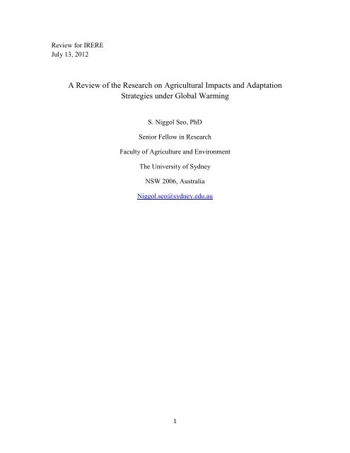
In contrast to the AEMs which are based on the experiments conducted on a selected
site, behavioral models randomly sample farm households from a large geographical area
such as the entire African continent. In Figure 1, we map the locations of household
surveys undertaken across Africa by the World Bank project in Africa (Dinar et al. 2008,
Seo et al. 2009, Seo 2012b). The figure draws the five Agro-Ecological Zones (AEZs)
defined by Dudal and the Food and Agriculture Organization (FAO) of the United
Nations: deserts, arid, semi-arid, sub-humid, and humid zones (Dudal 1980, FAO 2005).
The AEZs are classified based on the Length of Growing Periods for crops (LGP).
Household surveys, as shown by the black dots, are collected from all the AEZs and 11
countries from western Africa, central Africa, eastern Africa, southern Africa, and
northern Africa.
[Figure 1 around here]
In contrast to the AEMs which are necessarily constrained to major grains such as
wheat, maize, rice, and soybeans, the behavioral models include all the major and minor
grains, vegetables, oil seeds, fruits, tree products, and numerous animals and animal
products that are managed across the entire region of the concern. In addition, variations
of farm portfolios across commercial farming, family farming, and subsistence farming
are all modeled. That is, the behavioral method enables researchers to investigate the full
array of farm portfolios in the agriculture of a concerned region.
Summing up, since the behavioral approach is conducted at a micro level, covers a full
array of geography and ecosystems, includes a full array of farm portfolios, and
quantifies explicitly adaptation behaviors and profits, this approach was named as a G-
9

MAP model (a Geographically scaled Microeconometric model of Adapting Portfolios in
response to climate change), which further connotes a guide map for adaptations to
climate change.
Henceforth, a brief description of the G-MAP model is provided (Seo 2010b). A farmer
n is assumed to choose one of the agricultural systems (j) to maximize net revenue, given
climate and soils. That is, her problem is ArgMax π , π ,..., π } . Let the profit from
10
j{
n1
n2
nJ
agricultural system j and 1 be written as the sum of the observable component and the
unobservable component while the former can be written as a linear function of the
parameters as follows (Dubin and McFadden 1984):
π = X β + u
(1a)
n1
n 1 n1
π * = γ + η , j = 1,
2,...,
J.
(1b)
nj
where
Z n j nj
2
( un
1 | X , Z)
= 0,
Var(
u 1 | X , Z)
= σ .
(1c)
E n
The subscript j is a categorical variable indicating the choice amongst J agricultural
systems: j=1 denotes a specialized crop system, j=2 an integrated system, and j=3 a
specialized livestock system. The vector Z represents the set of explanatory variables
relevant for all the alternatives and the vector X contains the determinants of the profit of
the first alternative.
Assuming η j 's
are iid Gumbel distributed (McFadden 1974) and spatial neighborhood
effects are controlled by re-sampling from the neighborhoods (Anselin 1988, Case 1992,
Seo 2011b), the choice probability can be written as the sample average of the Logit
probabilities:
P
n1
= K
∑
k=
1
exp( Z γ )
n
n
1
exp( Z γ )
k
Having chosen agricultural system 1, the farmer makes numerous decisions regarding
inputs, outputs, and practices to maximize the expected profit from managing the system.
As profits are observed only for the farms that actually chose agricultural system 1,
selection biases are corrected to obtain consistent estimates of the parameters in the profit
equations (Heckman 1979). Following Jeffrey Dubin and Daniel McFadden (1984) for a
multinomial choice model, researchers assume a standard linearity condition with the
correlations among the alternatives ( λ ) summing up to zero. The conditional land value
(or profit) function for the first alternative is estimated as follows:
(2)

J ⎡ Pnk
⋅ ln P ⎤
nk
π n1
= X nϕ1
+ σ ⋅∑
λk
⋅ ⎢ + ln Pn1
⎥ + δ
k≠1
⎣ 1−
Pnk
⎦
In the above equation, δ is a white noise error term. Explanatory variables are climate
(either satellite based or high resolution climatology), soils, topology, hydrology (water
flows and runoff), market access (travel hours to major markets), household
characteristics, and country dummies which are obtained from the various geographically
references data sources (New et al. 2002, FAO 2003, Strezpek and McCluskey 2006,
Mendelsohn et al. 2007, World Bank 2009b). The choice equations are identified by the
variables that affect the choices, but not profit functions (Fisher 1966). The land values
for the specialized livestock system and the mixed system are estimated in the same
manner.
From the estimated probabilities in equation 2 and the conditional land values (profits)
for different systems in equation 3, the expected land value (profit) of the farm (n) is
calculated as the sum of the probability of each agricultural system times the conditional
profit of that system across the three systems given the external conditions including
climate (C) as follows:
J
Wn ∑ nj
nj
j=
1
( C)
= P ( C)
* π ( C)
(4)
The change in welfare, ΔW, resulting from a climate change scenario can be measured
as the difference in W after and before climate change. The change in the expected farm
profit captures both the changes in the probability that a farm will be a particular system
and the changes in the conditional profit that it would generate as that system.
Uncertainties of the estimates in the probabilities (eq. 2), in the system specific land
values (eq. 3), and in the expected farm land value (profit) are obtained from
bootstrapping the estimates by randomly sampling a large number of times from the
original sample and calculating the standard deviation and the 95% confidence intervals
(Efron 1979).
4. Findings from Agro-Economic Models
The Agro-Economic Models build upon the results from the controlled experiments
conducted by agronomists and climate scientists. All the AEMs rely on a set of selected
crop simulation models because they are calibrated to include all the factors that affect
crop yields including CO2 (Tubiello and Ewert 2002). The FACE (Free-Air CO2
Enrichment) experiments which better replicate the field conditions have been conducting
such experiments since the early 1990s when it was first conducted at the Duke Forest.
11
n1
(3)

The results from the 15 year FACE experiments as well as crop simulation models are
summarized in Table 1. The table shows average changes in the corresponding indicators
of crop growth from the numerous FACE studies when CO2 level is elevated to 2 times
the current level (Ainsworth and Long 2005). Major crops all increase in yields. On
average, rice yield increases by 10%, wheat yield by 15%, cotton yield by 42%, and
sorghum yield by 5% (by 40% under no stress) under the FACE experiments. Legumes
(soybeans) increase by 24% in dry matter production.
[Table 1 around here]
The fourth column of Table 1 summarizes the results from three crop simulation models
which were taken from Francisco Tubiello and his coauthors (Tubiello et al. 2007). The
AEZ model results are almost identical to the FACE experiment results. CERES and
EPIC models predict slightly higher yield increases. For example, rice yield increases by
10% under the FACE, but it increases by 17% under the CERES model and by 19%
under the EPIC model. The maize yield increases by 4% under the AEZ method, by 6%
under the CERES, and by 8% under the EPIC. Soybean yield increases by 16% under the
AEZ method.
Using the estimated yield changes obtained from the experiments, researchers estimate
the national level changes in the yields of the major crops under elevated CO2 conditions
and changed climates. For this purpose, researchers rely on the national agricultural
model such as the Agricultural Sector Model (ASM) of the US agriculture (Adams et al.
1990, 1999, Butt et al. 2005). Assuming the demand remains unchanged from the
baseline year (or gets updated over time), authors calculate the changes in agricultural
prices caused by yield changes due to climate change and CO2 elevation (Adams et al.
1990). Table 2 shows the changes in the Fisher price index from the baseline under the
two climate scenarios. The table shows the supply increase by 9% under the GISS
(Goddard Institute for Space Studies) scenario but decrease by 20% under the GFDL
(Geophysical Fluid Dynamics Laboratory) scenario. Accordingly, agricultural price index
falls by 17% under the GISS scenario and increases by 34% by the GFDL scenario.
[Table 2 around here]
By shifting the agricultural supply caused by climatic change, authors calculate the
changes in consumer surplus and producer surplus as well as total economic welfare.
Table 3 reports the results from the two GCM scenarios assuming 1981-1983 economy
(Adams et al. 1990). The total welfare increases by 11% under the GISS scenario while it
falls by 0.1% under the GFDL scenario. Under the GFDL scenario where yields fall
sharply and prices increase, consumers lose income substantially, but producers gain
income by 20% due to price increases.
[Table 3 around here]
12

Richard Adams and his coauthors have improved this model over time primarily in two
directions. First, they extended the analysis to non major cereals such as cotton-sorghum,
tomatoes-citrus-potatoes, and forage-livestock production (Adams et al. 1999, Reilly et
al. 2003). Forage yield changes were obtained from the EPIC crop simulation model for
the Southeast US and from the CENTURY model for the western US (Parton et al. 1992).
Based on the simulations on 17 sites in the Southeast and 12 sites in the Western US, the
ASM yield changes were estimated. From the pasture yield changes, the number of acres
required per head was estimated under the changed climate conditions. In addition, direct
effects of climate on cattle production on food intake (appetite depressing) were
estimated to calculate production efficiency using the NUTBAL model (Stuth et al.
1999). Putting all things together, authors estimated that the impacts of climate change on
livestock are negligible. The revised model is best summarized in the bottom panels of
Table 3 (Adams et al. 1999). Under the GFDL scenario, the impact is around 1% loss of
the total welfare in which 52 billion dollars of producer surplus is offset by the larger
losses by the consumers, domestically and internationally through export price increases.
In another direction, the original model was also applied to a non US country, e.g., Mali,
an arid zone country in the Sahel (Butt et al. 2005). Relying on the Mali Agricultural
Sector Model (MASM), authors find severe crop damages due to climate change as well
as livestock weight losses. However, they find that the impacts on the weights of goats
and sheep are not discernible while cattle weight decreases substantially due to both
decrease in forage quality and appetite.
The agro-economic modeling approach has been adopted widely for the past two
decades. Cynthia Rosenzweig and Martin Parry relied on a similar approach to measure
the impacts of climate change on global food supply (Rosenzweig and Parry 1994, Parry
et al. 2004). Crop simulations from the 18 countries around the world are used for wheat,
maize, soybeans, and rice. Site specific yield changes are aggregated to the national
levels. Based on the results from the 18 countries and 4 major crops (wheat, rice, maize,
soybeans), authors extrapolated to the yield changes in the rest of the world as well as to
the all the other crops raised across the world. Using the Basic Linked System (BLS)
composed of a set of linked national agricultural models, authors then simulated the
world food trade. Trades of grains among the world regions and their prices were
modeled (Tobey et al. 1992, Reilly et al. 1994). This approach was further refined by
incorporating varied crop potentials of different Agro-Ecological Zones (AEZ) around
the world using the FAO Global AEZ (GAEZ) data set (Fischer et al. 2005, FAO 2005).
However, it is likely that these models are less accurate than the US model since
extrapolations to the other crops, to the national agricultures, and to the other countries in
the world will likely involve substantial distortions.
13

5. Findings from the G-MAP Models
Behavioral models examine the full sets of farm portfolios which are composed of
numerous crops, livestock species, and forest products. The G-MAP model was first
applied to the animal species choice in Africa (Seo 2006, Seo and Mendelsohn 2008).
Figure 2 shows the changes in farmers’ choice probabilities of beef cattle, dairy cattle,
goats, sheep, and chickens across the range of temperature observed in Africa. It shows
beef cattle and dairy cattle choices fall sharply as temperature becomes hotter. On the
other hand, goats and sheep are increasingly chosen more often in the hotter zones of
Africa. Chickens reveal a hill shaped response in which the peak occurs at around the
mean temperature of the continent. The analysis also reveals that the choices of cattle and
sheep fall sharply when climate becomes wetter (because of more rainfall) while goats
and chickens are chosen more often when there is more rainfall.
[Figure 2 around here]
A broader agricultural model was developed subsequently. Depending upon whether the
farm owns crops or livestock or both, agricultural portfolios can be classified into a
specialized crop system, a specialized livestock system, and an integrated system that
owns both crops and livestock (Seo 2010a, 2010b, 2011b). For the illustration of the
results from the behavioral models, we will use the applications of the G-MAP model to
the South American agriculture and the African agriculture. As shown in Table 4, if
climate is changed according to the CCC (Canadian Climatic Center) A1 scenario by
2060, the crops-only system falls by 4.1%. The loss is offset by the increase in the
integrated system by 2.1% and in the livestock only system by 2% in South America (Seo
2010b). Under the UKMO (United Kingdom Meteorology Office) HadGEM1 A2
scenario, a crops-only farm falls by 1.6% and a specialized livestock farm falls by 0.6% 2
.
These decreases are offset by the increase in integrated farming by 2.1%. In Africa,
similar results are found (Seo 2011b). Under the PCM (Parallel Climate Model) scenario
which predicts a milder temperature increase and a rainfall increase in Africa, the
specialized crop system increases.
[Table 4 around here]
Given the choice of one of the agricultural systems, a farmer chooses a vector of inputs,
outputs and farm practices to maximize the expected return from the chosen system. In
estimating the land value of each system, selection biases are corrected. The empirical
results indicate that selection biases are large and the omission of them can lead to
strongly biased results (Seo 2010b). In addition, selection terms indicate the difference
between specialized farms and diversified farms. For example, the land value of the
2 The UKMO results are from the limited sample analysis which reported the exact GPS locations.
14

specialized crop system is lower when the farm is observed to have chosen the mixed
system, and vice versa.
After correcting for selection biases, Table 5 calculates the consistent impacts of climate
change on the three agricultural systems in South America (Seo 2010b). If the CCC
scenario comes to pass, the land value of the specialized crop system falls by 20% and
that of the specialized livestock system falls by 26%. But, the land value of the mixed
crop-livestock falls only by 9%. Under the UKMO (United Kingdom Meteorological
Office) HadGEM1 (Hadley Global Environmental Model) A2 scenario (Gordon et al.
2000), the land values of the crops-only and the livestock-only fall by 28.5% and 47.7%
respectively. Land value of the mixed farm is more resilient with 12.5% reduction in the
land value. In Africa, the results indicate even larger damage to the crops-only system,
but a similar resilience of the integrated farming (Seo 2010a).
[Table 5 around here]
Agricultural impact of climate change can then be calculated by combining both the
changes in agricultural portfolios and the changes in the conditional land values. Table 6
shows that agricultural damage from the CCC scenario in South America is 8.7% loss of
the land value (Seo 2010b). If UKMO A2 scenario is used, the damage amounts to 17%
of the land value. In Africa, the impact of climate change under the CCC scenario is
estimated to be around 9% loss of the agricultural profit when all the necessary
adaptation measures are taken. Under a milder and wetter PCM scenario, African
agriculture benefits from climate change since more rainfall benefits African farmers on
the arid zones and mostly rainfed (Seo 2010a).
[Table 6 around here]
The G-MAP model enables researchers to measure the impacts of climate change when
adaptations are not taken or cannot be taken due to various constraints by farmers even
though climate has changed. This implies the G-MAP analysis can put restraints on the
assumption of perfect foresight by the farmers. The damage under the CCC scenario
increases to 18% in South America. Under the UKMO A2 scenario, it increases to 19%
(Seo 2010b).
6. Adaptation Strategies to Climate Change
Having discussed the major findings from the two modeling approaches, we are well
positioned to discuss adaptation strategies to climate change and how to model them.
Adaptation is defined as behavioral adjustments in response to climatic changes,
therefore is a broader concept than the physical adaptation of the plants and animals to
15

climate which is studied by scientists (Easterling et al. 2007, Hoffmann 2010). Indeed,
the key distinction between the AEMs and the G-MAPs lies in the ways how adaptation
behaviors are modeled. The two methods differ fundamentally in that the AEMs are well
suited (intended) for understanding the changes in crop yields and their economic impacts
while the G-MAPs are designed for understanding the behavioral changes that occur at
the farm and their economic consequences. The base unit is a crop for the AEMs while it
is a farmer for the G-MAPs.
The AEMs can be effectively linked to agronomy, i.e., crop experiments which are
conducted locally (Jones and Kiniry 1986, Williams et al. 1989, Tubiello and Ewert
2002). The experiments are conducted on a selected site (plot). The G-MAPs are
effectively linked to the large scale geography such as the African continent and the
South American continent. Hence, the latter can be effectively linked to the ecosystem
sciences and ecology (Matthews 1983, Joyce et al. 1995, Schlesinger 1997, Gitay et al.
2001, Sankaran et al. 2005, Ainsworth and Long 2005, Fishlin et al. 2007). The G-MAPs
are effective in associating the choices of varied agricultural portfolios by farmers with
the underlying changes in agro-ecosystems (Seo 2010c, Seo 2012a).
The G-MAPs can account for the full array of adaptive adjustments and possibilities
when faced with climatic changes. In the model, farmers are allowed to adopt a different
species of animals or crops (Seo and Mendelsohn 2008a), Farmers are allowed to select a
certain enterprise or drop it when climate is altered. Selection bias which underpins the
core of the micro-econometrics literature can be explained in the G-MAP models
(Heckman 1979, Dubin and McFadden 1984, Seo 2010a, 2010b). Farmers may diversify
their portfolios or specialize into a certain portfolio (Markowitz 1952, Tobin 1958, Seo
2010a). Farmers can choose an integrated farming system. The G-MAPs are allowed to
account for spatial spillovers and neighborhood influences (Anselin 1988, Case 1992, Seo
2011b). The AEMs, on the other hand, have limited capacity in explaining the farmer’s
adaptive behaviors and social interactions.
Adaptation to increased climate uncertainties and risks is one of the key questions facing
the agricultural sector’s capacity to cope with climate change. The G-MAPs draw on the
long tradition of behavioral economic studies of risks and uncertainties in the financial
decisions and farm managements (Arrow 1971, Arrow and Fisher 1974, Kahneman and
Tversky 1979, Udry 1995, Zilberman 1998, Nordhaus 2011). A G-MAP model shows
that farmers in sub-Saharan Africa react to climatic risks caused by increased variations
in rainfall and temperature by adjusting agricultural portfolios (Seo 2012b). In the AEM
models, accounting for climate risks and uncertainties is challenging and few attempts
have been made to date.
Finally, the AEMs provide estimates of price changes of individual crops as well as of an
aggregate price index by simulating the supply and demand curves within the ASM
16

framework (Adams et al. 1990, Cline 1996). The G-MAPs account for a farmer’s
expectations of prices into the future. That is, land value is the present value of the stream
of expected net returns (rents) from the land over time (Mendelsohn et al. 1994). If
climate is altered, farmers adjust expectations of future returns and agricultural prices
from the land, which lead to behavioral changes.
7. Discussions: Yields, Weather, Risks, Regions, and Vulnerabilities
Some of the major researches that do not fall exactly into one of the two research
methods have been widely read and contributed significantly to the discussions in the
field. Studies that focus on the yield changes of selected crops have been popular. Many
of the crop yield studies that were conducted experimentally across different parts of the
world are summarized in the IPCC Third Assessment Report (Gitay et al. 2001). Three
crop classes and six land classes defined by the length of growing seasons were used to
solve globally for a computable general equilibrium model (Darwin 2004). Crop yield
changes in the dryland grain production systems in Montana in the United States were
matched with the CENTURY crop model after accounting for spatial heterogeneity of the
sub-regions and simulating the choice of crops at the field level (Antle et al. 2004).
Researchers examined yield changes econometrically using the aggregated (at the US
county level) yield information compiled by the USDA across the range of agro-climatic
zones in the US (Schlenker and Roberts 2009). Researchers examined the changes in the
yields of major crops at the global level using the historical data from 1980 and
associated them with historical climate changes (Lobell et al. 2011). Yield changes in
Africa were also associated with the changes in ENSO (El Nino Southern Oscillation)
and NAO (North Atlantic Oscillation) indices over time (Stige et al. 2006). The combined
impact of Asian Brown Clouds and greenhouse gases was examined in Indian rice
production using aggregated (at the state level) harvest data over time since 1960 to 2000
(Auffhammer et al. 2006).
Of these, the Wolfram Schlenker and Michael Roberts’s study has attracted much
attention for several reasons. The authors reported that cereal yields in the US would
decline, when accounting for nonlinear yield responses, by as much as 30-46% by 2100
under the mild climate change scenario (B1) and 63-82% under the severe warming
scenario (A1F1) (Schlenker and Roberts 2009). Table 7 summarizes mean yield impacts
for corn, soybeans, and cotton under the Hadley climate model predictions by 2070-2099.
Authors argued that the large yield losses are expected due to nonlinear (non-symmetric,
more appropriately) yield responses to temperature. They argued that the decline after the
peak is much steeper than the incline before the peak if a crop yield is estimated using a
non-parametric method. These predictions are largely at odds with the experimentally
based crop yield studies (Ainsworth and Long 2005, Tubiello et al. 2007) and perhaps
17

with the crop yield response functions known to agronomists (IPCC 1990). The
Schlenker and Roberts’s paper and their African yield paper (Schlenker and Roberts
2009, Schlenker and Lobell 2010), however, do not address a farmer’s selection
decisions, hence suffer from selection bias (Heckman 1979, Seo 2010a, 2010b).
[Table 7 around here]
Studies that focus on the net revenue or land value have also been applied widely across
the world from the US to India, Canada, Sri Lanka, Africa, Brazil, South America, and
China (Mendelsohn et al. 1994, Maddison 2000, Kumar and Parikh 2001, Reinsborough
2004, Seo et al. 2005, Schlenker et al. 2005, Kurukulasuriya et al. 2006, Timmins 2006,
Kurukulasuriya and Ajwad 2007, Seo and Mendelsohn 2008b, Sanghi and Mendelsohn
2008, Wang et al. 2010). In these studies which can be broadly classified as the Ricardian
approach developed by Robert Mendelsohn, William Nordhaus, and Daigee Shaw
(Mendelsohn et al. 1994), adaptations are implicit. Using the aggregated farm profit data
from the USDA Census and focusing on the five states of the Midwest US, researchers
calculated adjustment costs of the ‘median farmer’ in adapting to climate change by
applying the Bayesian rule to update priors on climate change and found that the
adjustment costs are rather small (Kelly et al. 2005). A panel data analysis for the US
agriculture was developed to explain the changes in net revenues and grain yields in
response to yearly weather fluctuations using the US county data (Deschenes and
Greenstone 2007).
Of these, the Olivier Deschenes and Michael Greenstone’s approach is worth noting in
which the authors constructed the panel data of net revenues and yields of the major crops
obtained from the USDA Census of Agriculture in 1978, 1982, 1987, 1992, 1997, and
2002 (Deschenes and Greenstone 2007). After constructing the panel data at the US
county level, authors measured the changes in the net revenues and grain yields in
response to deviations of temperature and rainfall conditions in a given year from the
long-term average weather. Authors found that the US famers cope well with the yearly
fluctuations of weather, predicting only minor changes in the agricultural profits and
yields due to climate changes in the future. As shown in Table 8 below, the authors find
that agricultural profits, corn yield, and soybean yield increase insignificantly by the end
of this century under the Hadley scenario. The results imply that yearly weather impacts
on agriculture are modest in the US owing to various technological options and financial
systems available in the advanced economy as well as the post-harvest physical storage
capacity (Udry 1995, Wright 2011). These results are by and large consistent with the
past studies on African farmers who are found to cope with weather shocks through
saving and storage of grains (Udry 1995, Kazianga and Udry 2006). From another
perspective, the results imply that a prolonged shift in weather, i.e., a climate shift, is
what would inflict farmers in the decades to come when such shifts are realized,
especially in the low-latitude developing countries.
18

[Table 8 around here]
The literature review so far showed that the impacts of climate change are more severe in
the low-latitude developing countries such as Africa and South America than in the
temperate zone countries such as the US. Literature has long supported that regional
vulnerabilities of agriculture as well as risk factors are varied (Reilly et al. 1996). Sub-
Saharan African countries are highly vulnerable because the region is already hot and
highly variable in climate; large areas are in deserts, arid, and semi-arid zones;
dependence on agriculture is very high (Downing 1992, Butt et al. 2005, Kurukulasuriya
et al. 2006, Seo et al. 2009, Hassan 2010, Seo 2010a). In South America, increases (or
decreases) of the grasslands, including the Pampas, the Brazilian Cerrados, and the
Venezuelan/Colombian Llanos, and the Amazon rain forests are at the center of the
regional vulnerabilities as well as the impacts on the vast ranges of the Andes mountains
where most smallholder farms are located (Viglizzo et al. 1997, Baethgen 1997, Magrin
et al. 1997, 2007, Rosenzweig and Hillel 1998, Seo and Mendelsohn 2008b, Seo 2010b,
2012a). In South and Southeast Asia, regional vulnerability hinges on the impacts of
climate change on rice production which is the primary staple crop in the region, the
abilities of farmers to diversify into specialty crops and forest products, and the melting
of the Himalayan glaciers in the long-term (Kumar and Parikh 2001, Aggarwal and Mall
2002, Seo et al. 2005, Auffhammer et al. 2006, Sanghi and Mendelsohn 2008, ADB
2009, Jacob et al. 2012). In Central Asia and North America, regional vulnerabilities
depend on the steppes and the prairies (Milchunas et al. 2005, Batimaa et al. 2008). In
Oceania, rangelands which account for about 70% of the Australian lands are key
vulnerability zones to climate change, given the backdrop of prolonged droughts and
heavy rainfall that alternate caused by the ENSO events (Campbell et al. 2000, White et
al. 2005, Seo and McCarl 2011). New opportunities and associated risks are expected to
rise as the formerly frozen lands become suitable for agriculture in the high latitude
countries including Canada and Russia (Easterling et al. 2007).
Agricultural vulnerability under a warming world depends, beyond agriculture, on
social, political, technological, and macroeconomic changes that will unfold in the future
which are uncertain (Downing 1992, Darwin et al. 2004, UN Population Division 2004,
FAO 2006). Establishments of property rights and political stability in Africa in the next
several decades may help improve food and agricultural security in the continent even
with increasing stresses from global warming (UN ECA 2005, Goldstein and Udry 2008).
Expansions of free trades and changes in national agricultural subsidies can significantly
alter agricultural landscapes around the world but may also help ameliorate the damages
from climate change on specific crops in specific regions (Tobey et al. 1992, Reilly et al.
1994, Darwin et al. 1995, Anderson 2009). The future demand for food depends on
population growth, consumption change, as well as changes of diet to meat or non-meat,
especially in developing countries (Delgado et al. 1999, UN Population Division 2004,
19

FAO 2006, 2009b). Advances in technology and institutions that underpinned the past
growth in agricultural production and the decline in prices through crop variety
improvements may continue but face increasing resource constraints such as available
land and marginal agro-climatic conditions (Evenson 2002, Evenson and Gollin 2003).
8. Future Directions
What does the future hold for the field of climate change and agriculture? This review
confirms that climatic changes in the next century and beyond will impose significant
stresses on agriculture and adaptation challenges will be high. Global climate policy
negotiations in the past decades indicate that agriculture will be part of the larger
discussions on mitigating greenhouse gases by, e.g., adopting carbon conserving
techniques, reducing methane emissions from animal husbandry, managing grasslands,
preserving and replanting forests, and productions of bio fuels (Antle and McCarl 2002,
Rajagopal et al. 2007, Smith et al. 2008, Thornton and Herrero 2010, Avetisyan et al.
2011, UNFCCC 2011a). A Green Climate Fund established from the recent United
Nations conferences has the goal of generating more than one billion US dollars annually
by 2020 which will be used to support adaptation programs in the vulnerable populations,
sectors, and regions (UNFCCC 2011b). A large fraction of the fund is expected to flow
into agricultural adaptations in low-latitude developing countries to support ‘climate
smart’ agriculture (World Bank 2011).
There is much less uncertainty on climate changes in the next half century than those in
the century’s end and beyond (IPCC 2007). Given this, researches must be directed to
climate adaptation programs which must be efficient at the local level (Seo 2010c,
2012a). Adaptation programs will turn out to be a cooperative process between the
farmers on the ground, extension service, researchers, and public and private agencies. As
climate is gradually changing in the near future, adaptation strategies may be directly
learned from the field observations of the changes in crop yields and farming practices in
response to changing climates. Researchers must heed to the vulnerabilities to and
adaptation possibilities to extreme weather events, increased climate risks, and
temperature thresholds which may (or may not) increase in frequency in the future among
the world regions (Easterling et al. 2000, Tebaldi et al. 2007, IPCC 2007, Schlenker and
Roberts 2009, Seo 2012b). Adaptation should be ideally taken by the affected individuals
who actually farm in the fields, but public adaptation supports are needed at various
levels of governance. Such supports should be carefully designed so as not to provide too
much of adaptation nor induce mal-adaptations (Seo 2011a). Research into new species
and varieties of crops and livestock may prove beneficial in the longer term as the
observed success stories have indicated, e.g., expansion of soybeans in the Brazilian
20

Cerrado and a heat tolerant Brahman cattle breed in India (Evenson and Gollin 2003,
Easterling et al. 2007, World Bank 2009, Hoffman 2010).
I conclude this review by looking forward to the distant future. My foresight tells me
that agriculture will continue to be at the heart of climate change discussions in this
century. The challenges ahead of us will be much greater than the scientific achievements
of the past decades. Climate changes will unfold expectedly and unexpectedly and the
impacts will be felt personally and increasingly more severely by the farmers.
Adaptations will take place, which significantly influence agricultural communities and
the society in general. Policy negotiations and implementations for the agricultural sector
at global, national, and local levels will turn out to be complex and an enduring process.
References
Adams, Richard, Cynthia Rosenzweig, Robert M. Peart, Joe T. Ritchie, Bruce A. McCarl,
J. David Glyer, R. Bruce Curry, James W. Jones, Kenneth J. Boote, and L. Hartwell
Allen, Jr. 1990. Global climate change and US agriculture. Nature 345: 219-224.
Adams, Richard, Bruce A. McCarl, Kathleen Segerson, Cynthia Rosenzweig, Kelly
Bryant, Bruce L. Dixon, Richard Conner, Robert E. Evenson, and Dennis Ojima.1999.
The economic effects of climate change on US agriculture. In Robert Mendelsohn and
James Neumann (Eds.) The Impact of Climate Change on the United States Economy.
Cambridge University Press, Cambridge. Pp. 18-54.
Adams, Richard M., Bruce A. McCarl, and Linda O. Means. 2003. Effects of spatial scale
of climate scenarios on economic assessments: An example from the US
agriculture. Climatic Change 60:131-148.
Aggarwal, P.K., and P.K. Mall. 2002. Climate change and rice yields in diverse agroenvironments
of India. II. Effect of uncertainties in scenarios and crop models on impact
assessment. Climatic Change 52: 331-343.
Ainsworth, Elizabeth A. and Stephen P. Long, 2005: What have we learned from 15
years of Free-Air CO2 Enrichment (FACE)? A meta-analysis of the responses of
photosynthesis, canopy properties and plant production to rising CO2. New
Phytology165: 351-372.
Amundson, J.L., Terry L. Mader, Richard J. Rasby, and Q.S. Hu. 2006. Environmental
effects on pregnancy rate in beef cattle. Journal of Animal Science 84: 3415-3420.
Anderson, Kym. 2009. Distortions to Agricultural Incentives: A Global Perspective,
1955–2007. World Bank, Washington DC.
21

Anselin, Luc. 1988. Spatial Econometrics: Methods and Models. Kluwer Academic
Publishers, Dordrecht.
Antle, John M. and Bruce A. McCarl. 2002. The economics of carbon sequestration in
agricultural soils. In T. Tietenberg and H. Folmer (Eds.) The International Yearbook of
Environmental and Resource Economics 2002/2003. Edward Elgar Publishing. Pp 278-
310.
Antle, John M., Susan M. Capalbo, Edward T. Elliott, and Keith H. Paustian. 2004.
Adaptation, spatial heterogeneity, and the vulnerability of agricultural systems to climate
change and CO2 fertilization: An integrated assessment approach. Climatic Change 64:
289–315.
Arrow, Kenneth J. 1971. Essays in the Theory of Risk Bearing, Chicago: Markham
Publishing Co.
Arrow, Kenneth J., and Anthony C. Fisher. 1974. Environmental preservation,
uncertainty, and irreversibility. Quarterly Journal of Economics 88: 312–319.
Asian Development Bank (ADB) 2009. Building Climate Resilience in the Agriculture
Sector in the Asia Pacific. Manila, the Philippines.
Auffhammer, Maximilian., V. Ramaathan, and Jeffrey R. Vincent. 2006. Integrated
model shows that atmospheric brown clouds and greenhouse gases have reduced rice
harvests in India. Proceedings of the National Academy of Science 103: 19668-19672.
Avetisyan, Misak, Alla Golub, Thomas Hertel, Steven Rose, and Benjamin Henderson.
2011. Why a global carbon policy could have a dramatic impact on the pattern of the
worldwide livestock production. Applied Economic Perspectives and Policy 33: 584-605.
Baethgen, Walter E. 1997. Vulnerability of agricultural sector of Latin America to
climate change. Climate Research 9:1-7.
Baker, B.B., J.D. Hanson, R.M. Bourdon, and J.B. Eckert. 1993. The potential effects of
climate change on ecosystem processes and cattle production on U.S. rangelands.
Climatic Change 23: 97-117.
Batimaa, P., L.Natsagdorj, and N.Batnasan.2008. Vulnerability of Mongolia’s pastoralists
to climate exterems and changes. In Neil Leary (Ed.) Climate Change and Vulnerability.
Earthscan, UK.
Butt, Tanveer A., Bruce A. McCarl, Jay Angerer, Paul T. Dyke, and Jerry W. Stuth.
2005. The economic and food security implications of climate change in Mali. Climatic
Change 68: 355–378.
22

Byerlee, Derek and Carl K. Eicher 1997. Africa’s Emerging Maize Revolution. Lynne
Rienner Publishers Inc, US. 301pp.
Campbell, B.D., D.M. Stafford Smith, A.J. Ash, J. Fuhrer, R.M. Gifford, P. Hiernaux,
S.M. Howden, M.B. Jones, J.A. Ludwig, R. Manderscheid, J.A. Morgan, P.C.D. Newton,
J. Nösberger, C.E. Owensby, J.F. Soussana, Z. Tuba, C. ZuoZhong. 2000. A synthesis of
recent global change research on pasture and rangeland production: reduced uncertainties
and their management implications. Agriculture, Ecosystems & Environment 82: 39-55.
Case, Anne. 1992. Neighborhood influence and technological change. Regional Science
and Urban Economics 22: 491–508.
Cline, William. 1992. The Economics of Global Warming. Institute of International
Economics, Washington DC.
Cline, William. 1996. The impact of global warming on agriculture: Comment. American
Economic Review 86: 1309-1311.
Consultive Group on International Agricultural Research (CGIAR). 2011. Mapping
Hotspots of Climate Change and Food Insecurity in the Global Tropics. CGIAR Research
Program on Climate Change, Agriculture and Food Security Report No. 5. Copenhagen,
Denmark.
Darwin, Roy. 2004. Effects of greenhouse gas emissions on world agriculture, food,
consumption, and economic welfare. Climatic Change 66: 191-238.
Darwin, R. F., M. Tsigas, J. Lewandrowski, and A. Raneses. 1995. World Agriculture
and Climate Change: Economic Adaptations. U.S. Department of Agriculture, Economic
Research Service, Washington, D.C.
Delgado, C., M. Rosegrant, H. Steinfeld, S. Ehui, and C. Courbois. 1999. Livestock to
2020: The next food revolution. Food, Agriculture, and the Environment Discussion
Paper 28, The International Food Policy Research Institute (IFPRI), Washington, D.C.
Dinar, Ariel, Rashid Hassan, Robert Mendelsohn, and James Benhin. 2008. Climate
Change and Agriculture in Africa: Impact Assessment and Adaptation Strategies.
EarthScan, London.
Dinar, Ariel, and Robert Mendelsohn. (Eds.) 2011. Handbook of Climate Change and
Agriculture. Edward Elgar: London.
Downing, Tom E. 1992. Climate Change and Vulnerable Places: Global Food Security
and Country Studies in Zimbabwe, Kenya, Senegal and Chile. Environmental Change
Unit, University of Oxford, Oxford.
23

Dubin, Jeffrey A. and Daniel L. McFadden. 1984. An econometric analysis of residential
electric appliance holdings and consumption. Econometrica 52: 345–362.
Easterling, David R., J.L. Evans, P. Ya. Groisman, T.R. Karl, K.E. Kunkel, and P.
Ambenje. 2000. Observed variability and trends in extreme climate events: a brief
review. Bulletin of American Meteorological Society 81: 417–425.
Easterling, William E., Pramod K. Aggarwal, Punsalmaa Batima, Keith Brander, Lin
Erda, MarkHowden, Andrei Kirilenko, John Morton, Jean-Francois Soussana, Josef
Schmidhuber, and Francisco N. Tubiello, 2007: Food, fibre and forest products. Climate
Change 2007: Impacts, Adaptation and Vulnerability. Contribution of Working Group II
to the Fourth Assessment Report of the Intergovernmental Panel on Climate Change,
M.L. Parry, O.F. Canziani, J.P. Palutikof, P.J. van der Linden and C.E. Hanson, Eds.,
Cambridge University Press, Cambridge, UK, 273-313.
Efron, B. 1979. Bootstrap methods: Another look at the Jackknife. Annals of Statistics 7:
1-26.
Evenson, Robert. 2002. Technology and Prices in Agriculture. In Consultation on
Agricultural Commodity Price Problems. Food and Agriculture Organization, Rome.
Evenson, Robert, and Douglas Gollin. 2003. Assessing the impact of the Green
Revolution 1960-2000. Science 300:758-762.
Fischer, Gunther, Mahendra Shah, Francesco N. Tubiello, and Harrij van Velhuizen.
2005. Socio-economic and climate change impacts on agriculture: an integrated
assessment, 1990–2080. Philosophical Transactions of the Royal Society B 360: 2067–
2083.
Fischlin, Andreas, Guy F. Midgley, Jeff Price, Rik Leemans, Brij Gopal, Carol Turley,
Mark Rounsevell, Pauline Dube, Juan Tarazona, Andrei Velichko. (2007) Ecosystems,
their properties, goods, and services. In: Parry ML, Canziani OF, Palutikof JP, van der
Linden PJ, Hanson CE (eds) Climate change 2007: Impacts, adaptation and
vulnerability. Contribution of Working Group II to the Fourth Assessment Report of the
Intergovernmental Panel on Climate Change Cambridge University Press, Cambridge.
Fisher, Ronald A. 1935. Design of Experiments. Oliver and Boyd: Edinburgh.
Fisher, Franklin M. 1966. The Identification Problem in Econometrics. McGraw-Hill,
New York.
Food and Agriculture Organization (FAO). 1978. Report on Agro-Ecological Zones
Project. Vol. 1. Methodology and Results for Africa. Rome.
24

Food and Agriculture Organization (FAO). 2003. The Digital Soil Map of the World
(DSMW) CD-ROM. FAO, Rome.
Food and Agriculture Organization (FAO). 2005. Global Agro-ecological Assessment for
Agriculture in the Twenty-first Century (CD-ROM). FAO Land and Water Digital Media
Series. FAO, Rome.
Food and Agriculture Organization (FAO). 2006. World Agriculture: Towards
2030/2050: Prospects for Food, Nutrition, Agriculture, and Major Commodity Groups.
FAO, Rome.
Food and Agriculture Organization (FAO). 2009a. Coping with a Changing Climate:
Considerations for Adaptation and Mitigation in Agriculture. FAO, Rome.
Food and Agriculture Organization (FAO). 2009b. The State of Food and Agriculture
2009: Livestock in the Balance. FAO, Rome.
Food and Agriculture Organization (FAO). 2012. FAO STAT. FAO Statistics Division,
Rome. Available at http://faostat.fao.org.
Ford, J. and K. Katondo. 1977. Maps of Tsetse fly (Glossina) distribution in Africa.
Bulletin of Animal Health and Production in Africa 15: 187-193.
Gitay, Habiba, Sandra Brwon, William Easterling, and Bubu Jallow. 2001. Ecosystems
and Their Goods and Services. In McCarthy et al. Climate Change 2001: Impacts,
Adaptations, and Vulnerabilities. Cambridge University Press, Cambridge, UK, pp. 237-
342.
Goldstein, Markus, and Christopher Udry. 2008. The profits of power: Land rights and
agricultural investment in Ghana. Journal of Political Economy 116: 981-1022.
Gordon, C., C. Cooper, C.A. Senior, H.T. Banks, J.M. Gregory, T.C. Johns, J.F.B.
Mitchell and R.A. Wood, 2000. The simulation of SST, sea ice extents and ocean heat
transports in a version of the Hadley Centre coupled model without flux adjustments.
Climate Dynamics 16: 147-168.
Hahn, G. LeRoy. 1981. Housing and management to reduce climate impacts on livestock.
Journal of Animal Science 52: 175-186.
Hahn, G. LeRoy. 1999. Dynamic responses of cattle to thermal heat loads. Journal of
Animal Science 77: 10–20.
Hanemann, W. Michael. 2000. Adaptation and its management. Climatic Change 45:
511-581.
25

Hassan, Rashid. 2010. Implications of climate change for agricultural sector performance
in Africa: Policy challenges and research agenda. Journal of African Economies 19: 77-
105.
Heckman, James J. 1979. Sample selection bias as a specification error. Econometrica 47:
153–162.
Hertel, Thomas W. and Stephanie D. Rosch. 2010. Climate change, agriculture, and
poverty. Applied Economic Perspectives and Policy 32: 355-385.
Hillel, Daniel, and Cynthia Rosenzweig. (Eds.) 2010. Handbook of Climate Change and
Agroecosystems: Impacts, Adaptation, and Mitigation. Imperial College Press, London.
Hoffmann, Irene. 2010. Climate change and the characterization, breeding and
conservation of animal genetic resources. Animal Genetics 41: 32-46.
Hulme, Mike, Ruth M. Doherty, Todd Ngara, Mark G. New, and David Lister. 2001.
African climate change: 1900–2100. Climate Research 17: 145–168.
Intergovernmental Panel on Climate Change (IPCC). 1990. Climate Change: The IPCC
Scientific Assessment, Cambridge University Press, Cambridge, UK.
Intergovernmental Panel on Climate Change (IPCC). 2001. The Physical Science Basis,
The Fourth Assessment Report, Cambridge University Press, Cambridge, UK.
Intergovernmental Panel on Climate Change (IPCC). 2007. The Physical Science Basis,
The Fourth Assessment Report, Cambridge University Press, Cambridge, UK.
Jacob, Thomas, John Wahr, W. Tad Pfeffer, and Sean Swensen. 2012. Recent
contributions of glaciers and ice caps to sea level rise. Nature. doi:10.1038/nature10847.
Jones, C.A. and J.R. Kiniry. 1986. CERES-Maize: A Stimulation Model of Maize
Growth and Development. Texas A&M University Press, College Station.
Johnson, Harold D. 1965. Response of animals to heat. Meteorological Monographs 6:
109-122.
Joyce, L.A., J.R. Mills, L.S. Heath, A.D. McGuire, R.W. Haynes, and R.A. Birdsey.
1995. Forest sector impacts from changes in forest productivity under climate change.
Journal of Biogeography 22: 703–713
Kahneman, Daniel, and Amos Tversky. 1979. Prospect theory: An analysis of decision
under risk. Econometrica 47, 263-291.
26

Kaiser, Harry M., Susan J. Riha, Daniel S. Wilks, David G. Rossiter, and Radha
Sampath. 1993. A farm-level analysis of economic and agronomic impacts of gradual
climate warming. American Journal of Agricultural Economics 75: 387-398.
Kazianga, Harounan, and Christopher Udry. 2006. Consumption smoothing? Livestock,
insurance, and drought in rural Burkina Faso. Journal of Development Economics 79:
413-446.
Kelly, David L., Charles D. Kolstad, and Glenn T. Mitchell. 2005. Adjustment costs from
environmental change. Journal of Environmental Economics and Management
50: 468–495.
Kumar, K.S. Kavi, and Jyoti Parikh. 2001. Indian agriculture and climate sensitivity.
Global Environmental Change 11: 147-154.
Kurukulasuriya, Pradeep, Robert Mendelsohn, Rashid Hassan et al., 2006. Will African
agriculture survive climate change? World Bank Economic Review 20: 367–388.
Kurukulasuriya, Pradeep, and Mohamed Ishan Ajwad. 2007. Application of the Ricardian
technique to estimate the impact of climate change on smallholder farming in Sri Lanka.
Climatic Change 81: 39-59.
Lobell, David, and Christopher B. Field. 2008. Estimation of the Carbon Dioxide (CO2)
fertilization effect using growth rate anomalies of CO2 and crop yields since 1961.
Global Change Biology 14: 39–45.
Lobell, David, Wolfram Schlenker, and Justin Costa-Roberts. 2011. Climate trends and
global crop production since 1980. Science 333: 616-620.
Maddison, David. 2000. A hedonic analysis of agricultural land prices in England and
Wales. European Review of Agricultural Economics 27: 519-532.
Mader, Terry L. 2003. Environmental stress in confined beef cattle. Journal of Animal
Science 81: 110-119.
Mader, T. L., and M.S. Davis. 2004: Effect of management strategies on reducing
heat stress of feedlot cattle: feed and water intake. Journal of Animal Science 82: 3077-
3087
27

Magrin , Graciela O., Maria I. Travasso, Raul A. Díaz, and Rafael O. Rodríguez. 1997.
Vulnerability of the agricultural systems of Argentina to climate change. Climate
Research 9: 31–36.
Magrin, Graciela, C. Gay Garcia, D. Cruz Choque, Juan C. Gimenez, Ana R.
Moreno, G.J. Nagy, Nobre Carlos, and Alicia Villamizar. 2007. Latin America. In: Parry,
M.L., O.F. Canzianni, J.P. Paultikof, P.J. van der Linden and C.E. Hanson (eds.) Climate
Change 2007: Impacts, Adaptation, and vulnerability: Contribution of Working Group II
to the Fourth Assessment Report of the Intergovernmental Panel on Climate Change.
Cambridge University Press, Cambridge, UK: 581-615.
Matsui , Tsutomu, Ofelia S. Namuco, Lewis H. Ziska, and Takeshi Horie. 1997. Effects
of high temperature and CO2 concentration on spikelet sterility in Indica rice. Field
Crops Research 5: 213–219.
Matthews, Elaine. 1983. Global vegetation and land use: New high-resolution data bases
for climate studies. Journal of Climate and Applied Meteorology 22: 474-487.
McFadden, Daniel L. 1974. Conditional Logit Analysis of Qualitative Choice Behavior.
In P. Zarembka (Ed.) Frontiers in Econometrics. Academic Press, New York, pp. 105-
142.
Mendelsohn, Robert, William Nordhaus, and Daigee Shaw. 1994. The impact of global
warming on agriculture: A Ricardian analysis. The American Economic Review 84: 753–
771.
Mendelshon, Robert. 2000. Efficient adaptation to climate change. Climatic Change 45:
583–600.
Mendelsohn, Robert, Pradeep Kurukulasuriya, Alan Basist, Felix Kogan, and Claude
Williams. 2007a. Climate analysis with satellite versus weather station data. Climatic
Change 81:71-83.
Milchunas, D.G., A.R. Mosier, J.A. Morgan, D.R. LeCain, J.Y. King and J.A. Nelson,
2005. Elevated CO2 and defoliation effects on a shortgrass steppe: forage quality versus
quantity for ruminants. Agriculture, Ecosystems, and Environment 111: 166-194.
New, Mark, David Lister, Mike Hulme, and Ian Makin 2002. A high-resolution data set
of surface climate over global land areas. Climate Research 21:1-25.
Nin, Alejandro, Simeon Ehui, and Samuel Benin. 2007. Livestock productivity in
developing countries: an assessment, in Robert Evenson and Prabu Pingali (eds),
28

Handbook of Agricultural Economics, Volume 3., North Holland, Oxford, UK, pp. 2467–
2532.
Nordhaus, William. 1994: Managing the Global Commons. MIT Press, MA.
Nordhaus, William. 2011. The economics of tail events with an application to climate
change. Review of Environmental Economics and Policy 5: 240-257.
Olmstead, Alan L., and Paul W. Rhode. 2011. Adapting North American wheat
production to climatic changes, 1839-2009. Proceedings of the National Academy of
Sciences of the United States 108: 480-485.
Parry, Marry L., Cynthia P. Rosenzweig, A. Iglesias, M. Livermore, and Gunther Fischer.
2004. Effects of climate change on global food production under SRES emissions and
socioeconomic scenarios. Global Environmental Change 14, 53–67.
Parsons, D.J., A.C. Armstrong, J.R. Turnpenny, A.M. Matthews, K. Cooper and J.A.
Clark, 2001: Integrated models of livestock systems for climate change studies. 1.
Grazing systems. Global Change Biology 7: 93-112.
Parton, W.J., B. McKeown, V. Kirchner, and D. Ojima. 1992. CENTURY Users Manual.
Fort Collins, CO: Natural Resource Ecology Laboratory, Colorado State University.
Patterson, D.T. and E.P. Flint. 1980. Potential effects of global atmospheric CO2
enrichment on the growth and competitiveness of C, and C4 weed and crop plants. Weed
Science 28: 71-75.
Pearce, D.W., W.R. Cline, A. Achanta, S. Fankhauser, R. Pachauri, R. Tol, and P.
Vellinga. 1996. The social costs of climate change: Greenhouse damage and the benefits
of control. Climate Change 1995: Economic and Social Dimensions of Climate Change,
Intergovernmental Panel on Climate Change. Cambridge University Press, Cambridge.
183–224.
Polley, H.W., H.B. Johnson and J.D. Derner. 2003. Increasing CO2 from subambient to
superambient concentrations alters species composition and increases above-ground
biomass in a C3/C4 grassland. New Phytology 160: 319-327.
Porter, J.H., M. L. Parry, and T.R. Carter. 1991. The potential effects of climatic change
on agricultural insect pests. Agricultural Forest Meteorology 57: 221-240.
Porter, John R., and Mikhail Semenev. 2005. Crop responses to climatic variation.
Philosophical Transactions of the Royal Society B 360: 2021-2035.
29

Rajagopal, D., S.E. Sexton, D. Roland-Holst, and D. Zilberman. 2007. Challenge of
biofuel: Filling the tank without emptying the stomach? Environmental Research Letters
2: 1-9.
Reilly, John, N. Hohmann, and Sally Kane. 1994. Climate change and agricultural trade.
Global Environmental Change 4: 24-36.
Reilly, John, Walter E. Baethgen, F. Chege, S. Van de Geijn, L. Enda, Ana Iglesias, G.
Kenny, D. Patterson, J. Rogasik, R. Rotter, C. Rosenzweig, W. Sombroek, and J.
Westbrook. (1996). Agriculture in a changing climate: impacts and adaptations. Climate
Change 1995: Impacts, Adaptations, and Mitigation of Climate Change. R. Watson, M.
Zinyowera, R. Moss, and D. Dokken, Eds., Intergovernmental Panel on Climate Change
(IPCC), Cambridge University Press, Cambridge, UK, pp. 427–468.
Reilly, J., F. Tubiello, B. McCarl, D. Abler, R. Darwin, K. Fuglie, S. Hollinger, C.
Izaurralde, S. Jagtap, J. Jones, L. Mearns, D. Ojima, E. Paul, K. Paustian, S. Riha,N.
Rosenberg, and C. Rosenzweig. 2003. U.S. agriculture and climate change: New results.
Climatic Change 59: 43-69.
Reinsborough, Michelle J. 2003. A Ricardian model of climate change in Canada.
Canadian Journal of Economics 36: 21-40.
Rosenberg, Norman J. 1992. Adaptation of agriculture to climate change. Climatic
Change 21: 385-405.
Rosenzweig, Cynthia and Martin Parry. 1994. Potential impact of climate change on
world food supply. Nature 367, 133–138.
Rosenzweig, Cynthia, and Daniel Hillel. 1998. Climate Change and the Global Harvest:
Potential Impacts of the Greenhouse Effect on Agriculture. Oxford University Press,
Oxford, United Kingdom, pp. 324.
Samuelson, Paul. 1938. A note on the pure theory of consumers' behaviour. Economica
5:61-71.
Sachs, Jeffrey D. 2005. The End of Poverty: Economic Possibilities of Our Time.
Penguin Books, New York.
Sanghi, Apurva, and Robert Mendelsohn. 2008. The impacts of global warming on
farmers in Brazil and India. Global Environmental Change 18: 655–665.
Sankaran, Mahesh, Niall P. Hanan, Robert J. Scholes, Jayashree Ratnam, David J.
Augustine, Brian S. Cade,Jacques Gignoux, Steven I. Higgins, Xavier Le Roux, Fulco
Ludwig, Jonas Ardo, Feetham Banyikwa, Andries Bronn, Gabriela Bucini, Kelly K.
Caylor, Michael B. Coughenour, Alioune Diouf, Wellington Ekaya, Christie J. Feral,
30

Edmund C. February, Peter G. H. Frost, Pierre Hiernaux, Halszka Hrabar, Kristine L.
Metzger, Herbert H. T. Prins, Susan Ringrose, William Sea, Jorg Tews, Jeff Worden,
Nick Zambatis. 2005. Determinants of woody cover in African savannas. Nature 438:
846–849.
Schenkler, Wolfram, Michael Hanemann, and Anthony Fisher. 2005. Will US agriculture
really benefit from global warming? Accounting for irrigation in the hedonic approach.
American Economic Review 95: 395–406.
Schlenker, Wolfram, and Michael Roberts. 2009. Nonlinear temperature effects indicate
severe damages to crop yields under climate change. Proceedings of National Science of
Academy of the United States 106(37): 15594–15598.
Schlenker, Wolfram, and David Lobell. 2010. Robust negative impacts of climate change
on African agriculture. Environmental Research Letters 5: 1-8.
Schlesinger, William H. 1997. Biogeochemistry: An Analysis of Global Change (2nd
edn). Academic Press, San Diego, CA.
Seo, S. Niggol. 2006. Modeling Farmer Responses to Climate Change: Climate Change
Impacts and Adaptations in Livestock Management in Africa. Yale University. p218.
Seo, S. Niggol. 2010a. Is an integrated farm more resilient against climate change?: A
micro-econometric analysis of portfolio diversification in African agriculture? Food
Policy 35: 32-40.
Seo, S. Niggol. 2010b. A microeconometric analysis of adapting portfolios to climate
change: Adoption of agricultural systems in Latin America. Applied Economic
Perspectives and Policy 32: 489-514.
Seo, S. Niggol. 2010c. Managing forests, livestock, and crops under global warming: A
micro-econometric analysis of land use changes in Africa. Australian Journal of
Agricultural and Resource Economics 54 (2): 239-258.
Seo, S. Niggol. 2011a. An analysis of public adaptation to climate change using
agricultural water schemes in South America. Ecological Economics 70: 825-834.
Seo, S. Niggol. 2011b. A geographically scaled analysis of adaptation to climate change
with spatial models using agricultural systems in Africa. The Journal of Agricultural
Science 149: 437-449.
Seo, S. Niggol. 2012a. Adaptation behaviors across ecosystems under global warming: A
spatial microeconometric model of the rural economy in South America. Papers in
Regional Science. DOI: 10.1111/j.1435-5957.2012.00435.x
31

Seo, S. Niggol. 2012b. Decision making under climate risks: An analysis of sub-Saharan
farmers’ adaptation behaviors. American Meteorological Society.
Seo, S. Niggol, Robert Mendelsohn, and Mohan Munasinghe. 2005. Climate change and
agriculture in Sri Lanka: A Ricardian valuation. Environment and Development
Economics 10 :581-196.
Seo, S. Niggol, and Robert Mendelsohn. 2008a. Measuring impacts and adaptations to
climate change: A structural Ricardian model of African livestock management.
Agricultural Economics 38: 151-165.
Seo, S. Niggol, and Robert Mendelsohn. 2008b. A Ricardian analysis of the impact of
climate change on South American farms. Chilean Journal of Agricultural
Research 68:69-79.
Seo, S. Niggol, and Bruce McCarl. 2011. Managing livestock species under climate
change in Australia. Animals 1: 343-365.
Seo, S. Niggol, Robert Mendelsohn, Ariel Dinar, Rashid Hassan, and Pradeep
Kurukulasuriya. 2009. A Ricardian analysis of the distribution of climate change impacts
on agriculture across Agro-Ecological Zones in Africa. Environmental and Resource
Economics 43(3): 313-332.
Seo, S. Niggol, Bruce McCarl, and Robert Mendelsohn. 2010. From beef cattle to sheep
under global warming? An analysis of adaptation by livestock species choice in South
America. Ecological Economics 69: 2486-2494.
Shaw, M. Rebecca, Erika S. Zavaleta, Nona R. Chiariello, Elsa E. Cleland1,Harold A.
Mooney, and Christopher B. Field. 2002. Grassland responses to global environmental
changes suppressed by elevated CO2. Science 298: 1987-1990.
Smit, B., D. McNabb, and J. Smithers. 1996. Agricultural adaptation to climate variation.
Climatic Change 33: 7-29.
Smith, Joel. 1997. Setting priorities for adaptation to climate change. Global
Environmental Change 7: 251–264.
Smith, Pete, Daniel Martino, Zucong Cai, Daniel Gwary, Henry Janzen, Pushpam Kumar,
Bruce McCarl, Stephen Ogle, Frank O'Mara, Charles Rice, Bob Scholes, Oleg Sirotenko,
Mark Howden, Tim McAllister, Genxing Pan, Vladimir Romanenkov, Uwe Schneider,
Sirintornthep Towprayoon, Martin Wattenbach, and Jo Smith. 2008. Greenhouse gas
mitigation in agriculture. Philosophical Transactions of the Royal Society B 363: 789-
813.
32

Stige, Leif Christian, Jorn Stave, Kung-Sik Chan, Lorenzo Ciannelli, Nathalie Pettorelli,
Michael Glants, Hans R. Herren, and Nils Chr. Stenseth. 2006. The effect of climate
variation on agro-pastoral production in Africa. Proceedings of the National Academy of
Science 103: 3049-3053.
Strzepek, K. and A. McCluskey. 2006. District Level Hydroclimatic Time Series and
Scenario Analyses to Assess the Impacts of Climate Change on Regional Water
Resources and Agriculture in Africa. CEEPA Discussion Paper No. 13., Pretoria,
Republic of South Africa.
Stuth, Jerry W., M. Freer, H. Dove, and R.K. Lyons. 1999. Nutritional Management for
Free-Ranging Livestock. In H. Jung (Ed.). Nutrition of Herbivores. American Society of
Animal Science, Savoy, IL, pp. 696-751.
Sutherst, R.W. 1991. Pest risk analysis and the greenhouse effect. Review of Agricultural
Entomology 79: 1177-1187.
Tebaldi, Claudia, Katharine Hayhoe, Julie M. Arblaster, and Gerald E.Meehl. 2007.
Going to the extremes: An intercomparison of model-simulated historical and future
changes in extreme events. Climatic Change 82: 233–234.
Thornton, Philip K., and Mario Herrero. 2011. Potential for reduced methane and carbon
dioxide emissions from livestock and pasture management in the tropics. Proceedings of
the National Academy of Science of the United States of America 107: 19667-19672.
Timmins, Christopher. 2006. Endogenous land use and Ricardian valuation of climate
change. Environmental and Resource Economics 33:119-142.
Tobey, James, John Reilly, and Sally Kane. 1992. Economic implications of global
climate change for world agriculture. Journal of Agricultural and Resource Economics
17: 195–204.
Tubiello, Francisco N., and Frank Ewert. 2002. Simulation the effects of elevated CO2 on
crops: approaches and applications to climate change. European Journal of Agronomy 18:
57-74.
Tubiello, Francisco N., Jeffrey S. Amthor, Kenneth J. Boote, Marcello Donatelli, William
Easterling, Gunther Fischer, Roger M. Gifford, Mark Howden, John Reilly, and Cynthia
Rosenzweig. 2007. Crop response to elevated CO2 and world food supply. European
Journal of Agronomy 26: 215-223.
Udry, Christopher. 1995. Risk and saving in Northern Nigeria. American Economic
Review 85(5): 1287–1300.
33

United Nations (UN). 2000. United Nations Millennium Declaration. The UN
Headquarters, New York.
United Nations (UN) Population Division. 2004. World Population to 2300. Department
of Economic and Social Affairs, New York: United Nations.
United States Department of Agriculture (USDA), 2007. Census of Agriculture 2007,
Available at http://www.agcensus.usda.gov/Publications/2007/index.php.
United Nations Economic Commission for Africa (UN ECA). 2005. African Governance
Report 2005. UNECA, Addis Ababa, Ethiopia.
United Nations Framework Convention on Climate Change (UNFCCC). 1998. Kyoto
Protocol to the United Nations Framework Convention on Climate Change. Geneva,
Switzerland.
United Nations Framework Convention on Climate Change (UNFCCC). 2011a. The
Durban Platform for Enhanced Action. Durban, South Africa.
United Nations Framework Convention on Climate Change (UNFCCC). 2011b. Report
of the Transitional Committee for the Design of Green Climate Fund. Durban, South
Africa.
Viglizzo, E.F., Z. Roberto, F. Lertora, G. Lopez, and J. Bernardos, 1997. Climate and
land use change in field-crop ecosystems of Argentina. Agriculture, Ecosystems and the
Environment 66: 61–70.
Wang, Jinxia, Robert Mendelsohn, Ariel Dinar, Jikun Huang, Scott Rozelle, and Lijuan
Zhang. 2009. The Impacts of Climate Change on China’s Agriculture. Agricultural
Economics 40: 323-337.
White, Neil, Robert W. Sutherst, Nigel Hall, Patrick Whish-Wilson. 2003. The
vulnerability of the Australian beef industry to impacts of the Cattle Tick (Boophilus
microplus) under climate change. Climatic Change 61: 157-190.
Williams, J.R., C.A. Jones, J.R. Kiniry, and D.A. Spaniel.1989. The EPIC crop growth
model. Transactions of the American Society of Agricultural Engineers 32: 497-511
World Bank 2008. World Development Report 2008: Agriculture for Development.
World Bank, Washington DC.
World Bank. 2009a. Awakening Africa’s Sleeping Giant: Prospects for Commercial
Agriculture in the Guinea Savannah Zone and Beyond. World Bank and FAO,
Washington DC.
34

World Bank. 2009b. Africa Infrastructure and Country Diagnostics (AICD). Washington,
DC: World Bank. Available online at:
siteresources.worldbank.org/INTAFRICA/Resources/AICD_exec_summ_9-30-08a.pdf
(verified 19 Jan 2011).
World Bank. 2011. Climate-Smart Agriculture: Increased Productivity and Food
Security, Enhanced Resilience and Reduced Carbon Emissions for Sustainable
Development. World Bank. Washington DC.
Wright, Brian. 2011. The economics of grain price volatility. Applied Economic
Perspectives and Policy 33: 32-58.
Zilberman, David. 1998. Agricultural and Environmental Policies: Economics of
Production, Technology, Risk, Agriculture, and the Environment. SUNY-Oswego, NY.
Ziska, Lewis H. 2003. Evaluation of yield loss in field-grown sorghum from a C3 and C4
weed as a function of increasing atmospheric Carbon Dioxide. Weed Science 51: 914-
918.
35

Table 1: AEM1-Simulated Crop Yield Changes under 2*CO2
FACE Crop Simulation Models
Crops/plants Indicators Mean Changes Mean Changes
Rice Crop yield Around +10% +10%(AEZ)
+17%(CERES-C3)
+19%(EPIC-C3)
Wheat Crop yield +15%* +11%(AEZ)
+17%(CERES-C3)
+19%(EPIC-C3)
Cotton Crop yield +42%*
Sorghum Crop yield Around +5%
+40% (under no
stress)
36
+6%(CERES-C4)
+8%(EPIC-C4)
Maize Crop yield +4%(AEZ)
+6%(CERES-C4)
+8%(EPIC-C4)
Soybeans
Crop yield +16%(AEZ)
(Legumes)
Dry matter
production
+24%*
* denotes 95% Confidence.

Table 2: AEM2-Agricultural Commodity Price and Quantity Indices (Base=1.0)
Price Index Quantity Index
GISS with CO2 Doubling 0.83 1.09
GFDL with CO2 Doubling 1.34 0.80
The results are from Adams et al. (1990)
37

Table 3: AEM3-Economic Consequences of Climate Change on the US Agriculture
Consumers Producers Foreign
Surplus
Total
Adams et al. (1990): Assuming Demand and Technology Remain Unchanged
GISS with CO2 +12.03% +8.93% +11.45%
Doubling
GFDL with CO2 -17.96% +19.94% -0.11%
Doubling
Adams et al. (1999): Assuming 2060 Baseline
GISS with
Doubling
CO2 +20.6
billion$
+45.4 billion$ +50.6
billion$
+116.6 billion$
(around +7% of total
value of agriculture
sector)
GFDL with
Doubling
CO2 -65.7
billion$
+52.2 billion$ -3.4 billion$ -16.9 billion$
(around -1% of total
value of agriculture
sector)
38

Table 4: G-MAP1-Changes in Choices of Agricultural Systems under Climate Change
Crops only Crops and livestock
South America
39
Livestock only
Baseline 35.88% 41.99% 21.44%
∆CCC A1 Scenario -4.14% +2.10% +2.04%
∆UKMO A2 Scenario -1.59% 2.13% -0.55%
Africa
Baseline 40.2% 53.7% 6.0%
∆CCC A2 scenario -4.29% +4.05% +0.24%
∆PCM A2 scenario +0.15% -0.41% +0.25%
The results are from Seo 2010b, 2011b.

Table 5: G-MAP2-Changes in the Land Values (per Hectare) of the Agricultural Systems
Conditional on the Choices
Crops only Crops and livestock Livestock only
South America
∆CCC A1 Scenario -412.3*
-190.9*
-526.5*
(-20.3%)
(-9.4%)
(-25.9%)
∆UKMO A2 Scenario -810.79*
-233.46*
-332.31*
(-28.5%)
(-12.5%)
(-47.7%)
* denotes significance at 5% level. These results are from Seo 2010b.
40

Table 6: G-MAP3-Impacts of Climate Change on Agriculture
Scenarios
Absolute
Changes ($) % Changes 95% Lower CL 95% Upper CL
South America with Full Adaptation: Land Value per Farm
∆CCC A1 -156.5 -8.71% -527.8 214.9
∆UKMO A2 -351.4 -17.1% -392.17 -310.80
South America without Adaptation of Agricultural Systems: Land Value per Farm
∆CCC A1 -322.2 -17.9% -441.5 -220.8
∆UKMO A2 -400.5 -19.1% -438.18 -362.84
Africa with Full Adaptation: Net Revenue per Farm
∆CCC A2 -53.1 -9% -56.19 -50.13
∆PCM A2 +217.4 +37% +200.87 +234.07
The results are from Seo 2010a, 2010b.
41

Table 7: Yield Studies: Impacts from the Non-Parametric Yield Functions in the US
Corn (maize) Soybeans Cotton
2070-2099, Piecewise Linear
Hadley B1 scenario -43% -35% -38%
Hadley A1F1 scenario -82% -72% -72%
The results are mean changes approximately taken from the impact figure from Schlenker
and Roberts (2009).
42

Table 8: Weather Studies: Panel Fixed Effects Estimates of Profit and Yield Changes in
the US
Agricultural profits ($) Corn (yield) Soybeans (yield)
Baseline (2002)
8.67 billion 2.38 billion bushels
32 billion dollars
bushels
Hadley 2 (2070-2099) +1.29 billion dollars +0.01 billion
bushels
+0.02 billion bushels
The results are from Deschenes and Greenstone (2007).
43

Figure 1: African Household Surveys across Agro-Ecological Zones
44

Figure 2: Adopting Animal Species across Temperature in Africa (Left: beef cattle (top),
dairy cattle (middle), chickens (bottom); Right: goats (top), sheep (bottom))
B
e
e
f
c
a
t
t
l
e
D
a
i
r
y
c
a
t
t
l
e
C
h
i
c
k
e
n
s
1.00
0.75
0.50
0.25
1.00
0.75
0.50
0.25
1.0
0.8
0.6
0.4
0.2
0
0
0
12 14 16 18 20
Annual Mean Temperature (degC)
22 24 26 28 30 32
12 14 16 18 20
Annual Mean Temperature (degC)
22 24 26 28 30 32
12 14 16 18 20
Annual Mean Temperature (degC)
22 24 26 28 30 32
G
o
a
t
s
1.0
0.8
0.6
0.4
0.2
S
h
e
e
p
45
0
1.0
0.8
0.6
0.4
0.2
0
12 14 16 18 20 22 24 26 28 30 32
Annual Mean Temperature (degC)
12 14 16 18 20
Annual Mean Temperature (degC)
22 24 26 28 30 32
Note: For all the panels, the horizontal axis is annual mean temperature (in degC) and the
vertical axis is choice probability.