Chapter 2 Eigenvalues and eigenvectors

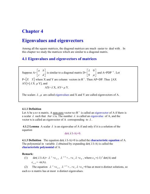
Chapter 4Eigenvalues and eigenvectorsAmong all the square matrices, the diagonal matrices are much easier to deal with . Inthis chapter we study the matrices which are similar to a diagonal matrix.4.1 Eigenvalues and eigenvectors of matrices⎡ab⎤⎡λ0⎤−1Suppose A= ⎢ ⎥ is similar to a diagonal matrix D= and A=PDP . Let⎣cd⎢ ⎥⎦⎣0µ ⎦2P=[ X Y ] where X and Y are column vectors in R . Then AP=DP. Thus [AXAY]=[ λ X µ Y], andAX= λ X, AY= µ Y.The scalars λ , µ are called eigenvalues and X and Y are called eigenvectors of A.4.1.1 DefinitionnLet A be a n×n matrix. A non-zero vector x∈R is called an eigenvector of A if there isa scalar λ such that Ax= λ x. The number λ is called an eigenvalue of A, and thevector x is called an eigenvector of A corresponding to λ .4.1.2 Lemma A scalar λ is an eigenvalue of A if and only if it is a solution of theequationdet( λ I-A)=0.4.1.3 Definition The equation det( λ I-A)=0 is called the characteristic equation of A.The polynomial in variable λ obtained by expanding det( λ I-A) is called thecharacteristic polynomial of A.Remark:(1) det( λ I-A)= λ n +ccn−1= -tr(A).n−1λ n −1n+...+c 1λ +c0, where c0=(-1) det(A) and(2) The equation λ n +cn−1λ n −1+...+c 1λ +c0=0has at most n distinct solutions, soeach n× n matrix has at most n distinct eigenvalues.

n(3) As det(A- λ I)= (-1) det( λ I-A), so λ is an eigenvalue iff it is a solution ofdet(A- λ I)=0.(4) In more advanced subjects, complex solutions of the characteristics equation are alsoaccepted as eigenvalues. In this course we only consider real eigenvalues.4.1.4 Theorem (Cayley-Hamilton) Ifλ n +cn−1λ n −1+...+c 1λ +c0=0is the characteristic equation of A, thennn−1A +cn−1A +...+c 1A+c0I=0,where I is the identity matrix.Exercise Verify the Cayley-Hamilton theorem by A, where⎡1−1⎤A= ⎢ ⎥ .⎣21 ⎦One application of the Cayley -Hamilton theorem is in computing powers of a givenmatrix.4.1.5 ExampleFind all the eigenvalues of A, where⎡01 0⎤A=⎢ ⎥⎢0 0 1⎥.⎢⎣4 −178⎥⎦Solution(i)The characteristic polynomial of A isdet( λ I-A)= λ 3 -8 λ 2 +17 λ -4.(ii) To solve λ 3 -8 λ 2 +17 λ -4=0 we first test if it has any integer solution.Every integer solution of a equation with integer coefficients must be a divisor ofthe constant term. By checking all the divisor 1,-1, 2,-2,4,-4, we find that 4 is a solution.Then divide the polynomial by λ -4, and writeλ 3 -8 λ 2 +17 λ -4=( λ -4)( λ 2 -4 λ +1).The remaining eigenvalues are the solutions ofλ 2 -4 λ +1=0,they are λ =2+ 3 and λ =2- 3 . So 4, λ =2+ 3 and λ =2- 3 are the eigenvalues ofA.

4.1.6 Definition Let λ 0be an eigenvalue of A. the solutions of the linear systemn( λ 0I-A)x=0 is a subspace of R ,it is called the eigenspace of A.RemarkIf λ 0is an eigenvalue, then ( λ 0I-A)x=0 must have a nonzero solution.thus the dimension of each eigenspace is nonzero.4.1.7 ExampleFind a basis for each of the eigenspaces of⎡0A=⎢1⎢⎢⎣1020− 2⎤1⎥⎥3 ⎥⎦Solution: The eigenvalues of A are λ =1 and λ =2. So there are two eigenspaces of A.(1) The eigenspace of A corresponding to λ =1 is the solution space of (2I-A)X=0, that is⎡ 1 0 2 ⎤ ⎡x⎤⎡0⎤⎢−1−1−1⎥ ⎢y⎥=⎢0⎥.⎢⎥ ⎢ ⎥ ⎢ ⎥⎢⎣−10 − 2⎥⎦⎢⎣z⎥⎦⎢⎣0⎥⎦The general solution of this system isx =-s,y =t,z =sSo S={ (-1,0,1), (0,1,0)} is a basis of the eigenspace correspondingto λ =2.(2) The eigenspace of A corresponding to λ =2 is the solution space of the linear system⎡ 2 0 2 ⎤ ⎡x⎤⎡0⎤⎢−10 −1⎥ ⎢y⎥=⎢0⎥.⎢ ⎥ ⎢ ⎥ ⎢ ⎥⎢⎣−10 −1⎥⎦⎢⎣z⎥⎦⎢⎣0⎥⎦The general solution of this system isx =-2s,y =s,z =s.Thus B={(-2,1,1)} is a basis for the eigenspace of Acorresponding to λ =1.

4.2 Diagonalizable matricesIn this section we investigate :(1) when a given matrix A is diagonalizable, and(2) how to find a matrix P that diagonalizes A.Recall that a square matrix is called a diagonal matrix if all its entries off the maindiagonal are zero.4.2.1 DefinitionA square matrix A is said to be diagonalizable if there is an invertible matrix P such−1that P AP is a diagonal matrix; the matrix P is said to diagonalize A.Thus A is diagonalizable if and only if A is similar to a diagonal matrix.4.2.2 TheoremIf A is a n×n matrix, then A is diagonalizable iff the sum of the dimensions of alleigenspaces of A is n.Question: Suppose A is diagonalizable. How to find D and P?4.2.3 Algrithm (Steps for finding P)Step 1 Find all eigenvalues of A, say λ 1, λ 2,…, λ r.Step 2 Find a basis for each of the eigenspaces.Step 3 If the sum of the dimensions of all eigenspaces is n then A is diagonalizable, andP is obtained by putting all vectors in each of the bases as column vectors.Step 4 Suppose q 1, q 2,...,qnare the vectors from all the bases corresponding to the−1eigenvalues µ 1, µ 2 2,…, µ n. Then P AP=D, where D is the diagonal matrixof which the entries on the main diagonal are µ 1, µ 2,…, µ n.4.2.4 ExampleLet

⎡00 − 2⎤A=⎢1 2 1⎥.⎢ ⎥⎢⎣1 0 3 ⎥⎦(1) Find P that diagonalizes A.(2) Find A 10 .Solution(1) A has two eigenvalues λ =1 and λ =2.The dimension of the eigenspace corresponding to λ =1 is 2 and that corresponding toλ =2 is 1. As 1+2=3, A is diagonalizable.{(-1,0,1),(0,1,0)} is a bases for the eigenspace of 1, and {(-2,1,1)} is a bases for theeigenspace of 2. Thus⎡−10 − 2⎤P=⎢0 1 1⎥⎢ ⎥⎢⎣1 0 1 ⎥⎦diagonalizes A, and⎡10 0⎤−1P AP=D=⎢0 1 0⎥.⎢ ⎥⎢⎣0 0 2⎥⎦−1So A=PDP .⎡10 0 ⎤(2)Thus A 10 =PD 10 −1P = P⎢ ⎥ −1⎢0 1 0⎥P .10⎢⎣0 0 2 ⎥⎦Remark The matrix P that diagonalizes A is not unique. In fact if P diagonalizes A,then any Q matrix obtained by rearranging the columns of P also diagonalizes A.4.2.5 Theorem If an n × n matrix A has n different eigenvalues, then A isdiagonalizable.4.2.6 Example Every triangular matrix with different entries on its main diagonal isdiagonalizable.

4.2.7 Definition Let λ 1be an eigenvalue of a matrix A. The dimension of theeigenspace corresponding to λ 1is called the geometric multiplication of λ 1, andthe number of times that λ - λ 1appears as a factor in the characteristic polynomial of Ais called the algebraic multiplicity of λ 1.4.2.8 Theorem Let A be a square matrix. Then(1) For any eigenvalue of A the geometric multiplicity is less than or equal to thealgebraic multiplicity.(2) A is diagonalizable if and only if the geometric multiplicity is equal to the algebraicmultiplicity for eacheigenvalue of A.Exercise 4.2⎡ab⎤⎡xz ⎤1. Let A= ⎢ ⎥ be diagonalized by P= such that⎣cd⎢ ⎥⎦⎣yw⎦−1 ⎡λ0⎤P AP= ⎢ ⎥ .⎣0µ ⎦(i) Verify that λ and µ are eigenvalues of A.⎡x⎤⎡ z ⎤(ii) Let u= ⎢ ⎥ and v= . Verify Au=λu and Av=µv.⎣ y⎢ ⎥⎦ ⎣w⎦2. (1) Find A 100 101and A , where⎡2− 3⎤A= ⎢ ⎥ .⎣1− 2⎦n(2) Find A for positive integer n, where⎡ 3 −10 ⎤A=⎢⎥⎢−12 −1⎥⎢⎣0 −13 ⎥⎦3. Show that if B={ u 1, u2,...,u k} consists of eigenvectors of ann× n matrix A, then the subspace span(B) is invariant undern nT : R → R , that isA

For each u in span(B), TA(u) is still in span(B).4.3 Eigenvalues and eigenvectors of linear operators (optional)4.3.1 DefinitionLet T: T: V → V be a linear operator on a vector space V.(i)A nonzero vector u in V is called an eigenvector of T if Tu=λu for some scalarλ. The scalar λ is then called an eigenvalue of T, and u is called an eigenvectorof T corresponding to λ.(ii) The eigenspace of T corresponding to an eigenvalue λ is the kernel ofλI -T: V →V.4.3.2 Proposition Let T:V→V be a linear transformation on a finite dimensional space Vand B is a basis for V. Then(1) The eigenvalues of T are the same as the eigenvalues of the matrix [T] .B(2) A vector u is an eigenvector of T corresponding to λ if andonly if its coordinator vector [u]Bis an eigenvector of [T]Bcorresponding to λ.4.3.3 ExampleLet T:P →P be the linear operator on P defined by2 2 22 2T(a+bx+cx )=(a+b+c)+(b+c)x+cx .Find all eigenvalues of T and a basis of the eigenspace for each eigenvalue.Solution:We chose to use the standard basis B={ 1,x,x 2 } of P2. The matrix of T with respect toB is⎡11 1⎤[T]B=⎢ ⎥⎢0 1 1⎥.⎢⎣0 0 1⎥⎦2A has only one eigenvalue λ=1. A polynomial p(x)=a+bx+cx is an eigenvector of Tcorresponding to λ=1 if and only if the vector [p(x)]B=(a,b,c) is a solution of the linearsystem(I-A)X=0.

The dimension of the eigenspace is 1, and S={(1,0, 0)} is a basis for the eigenspace.Thus the eigenvecotors of T with respect to λ=1 are all constant polynomials.4.3.4 Example Let D be the vector space of all infinitely differentiable functions definedon R, and δ : f(x) a f’(x) is the differentiation operator on D. Then for each real numberλ, we haveδ (e λ x)=λe λ x.λxThus every real number is an eigenvalue of δ , and the function e is an eigenvectorcorresponding to λ.Exercise 4.31. Let C[0,1] be the vector space of continuous real functions defined on [0,1]. DefineF: C[0,1] → C[0,1] byF(f(x)=xf(x), for all f(x) ∈C[0,1].(1) Prove that F is a linear operator.(2) Prove that F has no eigenvalue2. Prove: if a linear operator T:V → V is invertible then 0 is not an eigenvalue of T.