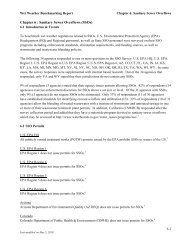
4500GHG Abated (kg CO2 eq.)4000350030002500200015001000500015 SEERStandard16 SEERStandard17 SEERStandard15 SEERStandard16 SEERStandard17 SEERStandardProcess LCA ResultsEIO‐LCA ResultsAnn ArborSan AntonioFigure 5.2: Potential GHG Avoided Using LCO under Different Federal Efficiency StandardScenariosThe optimal replacement results are shown for a 16 SEER CAC in Ann Arbor and San Antonio inTable 5.5 and Table 5.6. Results for the other efficiency scenarios are given in the Appendix.Table 5.5: LCO Results for Ann Arbor and San Antonio with an Updated 16 SEER StandardUsing Process LCI ResultsObjective Schedule <strong>Life</strong> <strong>Cycle</strong> Impacts % Deviation from theOptimumEnergy GHG (kg Cost Energy GHG Cost(MJ) CO2 eq.) (2009$)Ann Energy 1985, 1992, 1998, 1,047,000 89,600 26,500 ‐‐‐ 1.5 % 22.7 %Arbor2007, 2017GHG 1985, 1992, 2007, 1,051,000 88,200 24,400 0.4 % ‐‐‐ 12.6 %2017Cost 1985, 1995, 2008 1,084,000 89,100 21,600 3.6 % 1.0 % ‐‐‐SanAntonioEnergy 1985, 1989, 1992, 3,524,000 215,200 57,600 ‐‐‐ 1.9 % 26.4 %1998, 2006, 2007,2011, 2017City 1985, 1992, 2007, 3,570,000 211,300 47,100 1.3 % ‐‐‐ 3.5 %2017Cost 1985, 1995, 2008 3,709,000 217,400 45,600 5.3 % 2.9 % ‐‐‐
Table 5.6: LCO Results for Ann Arbor and San Antonio with an Updated 16 SEER StandardUsing EIO‐LCA Results aObjective Schedule <strong>Life</strong> <strong>Cycle</strong> Impacts % Deviation from theOptimumEnergy(MJ)GHG (kgCO2 eq.)Cost(2009$)Energy GHG CostAnnArborSanAntonioEnergy 1985, 1989, 1992, 1,024,000 91,700 32,100 ‐‐‐ 4.5 % 48.3 %1998, 2006, 2010,2017GHG 1985, 1992, 2007, 1,032,000 87,700 24,400 0.8 % ‐‐‐ 12.6 %2017Cost 1985, 1995, 2008 1,071,000 88,800 21,600 4.6 % 1.2 % ‐‐‐Energy 1985, 1988, 1989, 3,486,000 221,100 69,000 ‐‐‐ 4.9 % 51.5 %1992, 1995, 1998,2003, 2006, 2007,2010, 2016, 2017GHG 1985, 1992, 2007, 3,552,000 210,800 47,100 1.9 % ‐‐‐ 3.5 %2017Cost 1985, 1995, 2008 3,696,000 217,000 45,600 6.0 % 3.0 % ‐‐‐a) EIO‐LCA results refer to modeling <strong>of</strong> the unit production. See Section 3.1 for details.By comparing the optimal results for the energy and GHG objectives among the differentscenarios, it is evident that progressively higher efficiency standards from 15 SEER to 16 SEER to17 SEER will reduce environmental burdens over the time horizon. In the case <strong>of</strong> the GHGoptimization for Ann Arbor, a 15 SEER standard has no effect because the final replacementoccurs in 2010, before the new standard takes effect. This boundary effect would disappear ifthe time horizon was extended. In the 16 SEER scenario, the increase in efficiency andcorresponding reduction in GHG emissions during the use phase becomes large enough that it isbeneficial to replace after 2017 thus yielding a reduction in GHG emissions.The results from the efficiency scenario analysis are similar to those in the base case, which didnot account for a new efficiency standard. For instance, in the 16 SEER scenario, the energyobjective still requires the most replacements and as a result raises the cost dramatically. Withthe exception <strong>of</strong> going from 3 to 4 total units in order to minimize GHG emissions in Ann Arbor,the number <strong>of</strong> replacements does not change in these scenarios relative to the originalefficiency scenario.5.5 Impact <strong>of</strong> Carbon PriceTo evaluate the impact <strong>of</strong> potential carbon pricing, either in the form <strong>of</strong> a carbon tax or under acap and trade system, four different carbon costs were assigned to a ton <strong>of</strong> CO2 equivalentstarting in 2009 through 2025. This analysis assumed the full costs <strong>of</strong> carbon are ultimatelypassed on to the consumer and no portion <strong>of</strong> the carbon cost is absorbed by the manufacturer,contractor, or utility. The effect on the optimal cost solution is shown in Table 5.7.
- Page 4: Document DescriptionLIFE CYCLE OPTI
- Page 8 and 9: 4.3 Energy Intensity ..............
- Page 10 and 11: List of TablesTable 1.1: Cooling Lo
- Page 12 and 13: 1 IntroductionMechanical air condit
- Page 14 and 15: The overall demand for space coolin
- Page 16 and 17: Cooling is provided when the liquid
- Page 18 and 19: 2 Methodology2.1 Life Cycle Assessm
- Page 20 and 21: chart. Replacing a product with a m
- Page 22 and 23: Each component was assigned to an a
- Page 24 and 25: Indoor UnitThe indoor unit was assu
- Page 26 and 27: Index (10 SEER =1)2.502.001.501.000
- Page 28 and 29: Producer costs for higher and lower
- Page 30 and 31: Figure 3.6: North American Electric
- Page 32 and 33: Table 3.5: Summary of Bin‐Based M
- Page 34 and 35: 3.5 End‐of‐LifeIt was assumed t
- Page 36 and 37: RefrigerantsAs described in Section
- Page 38 and 39: 5 Results and Discussion5.1 Model A
- Page 40 and 41: 5.3 Comparing Optimal Replacement t
- Page 44 and 45: Table 5.7: Impact of Carbon Price o
- Page 46 and 47: Ann Arbor GHG$676 $1,188 $1,188Ann
- Page 48 and 49: emphasize sensible cooling capacity
- Page 50 and 51: Energy Star, the average premium fo
- Page 52 and 53: holding period for minimizing cost
- Page 54 and 55: 7.3 Policy ImplicationsThis researc
- Page 56 and 57: 8 BibliographyAHRI. (2008). 2008 St
- Page 58 and 59: Kim, H. C., Keoleian, G. A., & Hori
- Page 60 and 61: AppendixA.1 Energy IntensityMuch of
- Page 62 and 63: A.2 LCO Results of Standard Efficie
- Page 64 and 65: A.3 Comparison of Optimal to Typica
- Page 66 and 67: Table A.0.7: LCO Results for 16 SEE
- Page 68 and 69: Table A.0.9: LCO Results for 15 SEE
- Page 70 and 71: Table A.0.11: LCO Results for 17 SE
- Page 72 and 73: Table A.0.13: Comparison of Optimal
- Page 74 and 75: 2008 Energy 2008, 2012, 1,448,000 2
- Page 76 and 77: SouthCarolina1992 Energy(MJ)GHG(CO2
- Page 78 and 79: 2017Cost (2009$) 2003, 2013 $7,770
- Page 80 and 81: A.8 High Efficiency CAC Rebate Surv
- Page 82: Memphis Light, Gas and Water Memphi