An Introduction to the Ito Calculus and Stochastic Differential ...

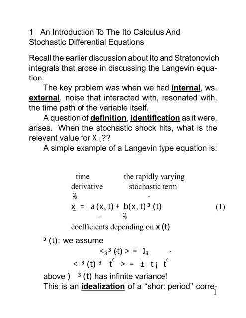
lated process.Example: =°2 e¡° jt¡t 0 jthe correlation function for the Ornstein-Uhlenbeck process.This is correlated, not a white noise process. But, thelimit of this as°!1 is a Divac delta function and is,in the limit, a white noise process.Thus:1R¡1°2 e¡° jt¡t 0 j definition of adt= 1 »Gausse Distributionlim°!1°2 e¡° jt¡t 0 j =0 8¯¯¯t¡t0¯¯¯6=0So a ‘white noise process ’can be regarded as thelimit of an Ornstein-Uhlenbeck process, with very fastinteraction, rather with very short correlation times.It seems reasonable in order to make equation (1)useful as a model to require:U(t)=Z t0³³t 0´dt 0exists and is continuousU(t) is then Markov:U(t), ¡ U ¡ t 0 ¢ ¡U(t)¢ , t0>tare independent.IfU(t) is continuous, it will have a Fokker-Planckrepresentation.2

We see in this case that:A(U 0 ,t)=0B(U 0 ,t)= 4t4t =1This is just the Wiener processZ t³³t 0´dt 0 = U(t) = W(t),in the old notation.0An alternative way of writing equation (1) is:x(t)¡x(0) =Z t0a[x(s),s]dstR h i+ b x(s)|{z} ,s ³(s)ds0%The key elementThis is an equation for the solution ofx(s) whichdepends on coefficients that in turn depend onX(s).Further, we have to worry about what X(s) in b[²] isused to multiply the effect of³(s) onX(s)!Traditionally, using the Wiener process interpretation:4

Z tb[x(s),s]³(s)ds )Z tb[x(s),s]dW(s)0This last equation poses the problem:We have to define what we mean by:tR h ib x(s)|{z} ,s dW(s)|{z }0. &stochastic process Wiener processdepending on aWiener process0(2)We will see that evenZ t0b(s)dW(s)needs interpretation forW(s), Wiener.The Gaussianity involved withdW(s) follows fromthe assumed continuity of U(t), coupled with theFokker-Planck expansion.1.1 Definition Of A Stochastic IntegralLetG(t)be an arbitrary continuous function. W(t)is aWiener process- independent Gaussian increments of 5

a continuous stochastic process, stationary with zeromean.Let us begin with a Rieman-Stieltjes integral interpretationof G(s)dW(s).tRt 0DiagramDefine¿ i 3t i¡1·¿ i·t i forft i g any partition of[t 0 ,t].We define the partial sum:S n =X ni=1G(¿ i )[W(t i )¡W(t i¡1 )]In the usual definition of the Rieman-Stieltjes integralnotinvolving a Wiener process- the partial sum limitdoes not depend on how the ¿ i are chosen inside[t i¡1 ,t i ].Here, it does.6

LetG(t)=W(t).We consider: =[min(¿ i ,t i )¡min(¿ i ,t i¡1 )]" "use of expectation + independent increments» CorrelationW(¿ i )W(t i )Therefore,=X ni=1(¿ i ¡t i¡1 ).Let¿ i = at i +(1¡a)t i¡1 , 0·a·1Therefore,< S n >=X ni=1(t i ¡t i¡1 )a= (t¡t 0 )a can be anything from0 to(t¡t 0 )!The Ito solution is to choosea=0; i.e. ¿ i = t i¡1 ,so that the functionG(t)is treated as non-anticipatingfor[W(t i )¡W(t i¡1 )].7(3)

We define the Ito Stochastic Integral:Z tGt 0³t 0´dW³t 0´´Recall:ms¡lim f P G(t i¡1 )[W(t i )¡W(t i¡1 )]gn! 1(4)ms¡lim X n =Xn! 1if and only iflim =0n! 1i.e. if and only ifZlimn! 1dwp(!)[X n (!)¡X(!)] 2 =01.1.1 A Key ExampleLetZ tt 0W(s)dW(s)W i =W(t i ), i=1,... n.8

S n =X nW i¡1 4W iW i¡1 (W i ¡W i¡1 ) = Xi=1 iWe solve this with a ‘trick ’re-exp.- Let ‘W i¡1 4W i ’ be the ‘cross-product ’termin a quadratic expansion.S n = 1 X n h(W i¡1 +4W i ) 2 :::2i=1i¡ (W i¡1 )| {z } 2 ¡(4W | {z i)}2. &Therefore, S n = 1 hW(t) 2 ¡W(t 0 ) 2i ¡ 1 2 2We now average:< X (4W i ) 2 >= X i=X ni=1(t i ¡t i¡1 ) =(t¡t 0 )This gives us the mean of P (4W i ) 2 ; we nowneed to see that its variance)0.Consider:X ni=1(4W i ) 29

=< X (W i ¡W i¡1 ) 4 +2 X i>j(W i ¡W i¡1 ) 2 (W j ¡W j¡1 ) 2¡2(t¡t 0 ) X (W i ¡W i¡1 ) 2 +(t¡t 0 ) 2 >W i ¡W i¡1 is Gaussian and is ind. of W j ¡W j¡1forjj(t i ¡t i¡1 )(t j ¡t j¡1 )¡2(t¡t 0 ) 2 + (t¡t 0 ) 2) 2 X (t i ¡t i¡1 ) 2 + X iX(t i ¡t i¡1 )(t j ¡t j¡1 )j:::) ¡(t¡t 0 ) 2 10

) X iXj[(t i ¡t i¡1 )¡(t¡t 0 )][(t j ¡t j¡1 )¡(t¡t 0 )]= 0by suming over one index first and recognizing thatX(ti ¡t i¡1 ) = (t¡t 0 ).The variance of P (4W i ) 2 is:2 X (t i ¡t i¡1 ) 2 · 2(t¡t 0 )" n ,since" n !0.Asn! 1, above)0 the limit.» the sum is on the µ order of122¢n¢ = 2 n n ! 0asn! 1.We conclude:a)ms¡lim P (4W i ) 2 =(t¡t 0 )n! 1b)Z tt 0W³t 0´dW³t 0´11

=the standard resultz }| {1hiW(t) 2 ¡W(t 0 ) 2 ¡(t¡t 0 )2| {z }enters because < P (4W i ) 2 > is ofsame order as rest of statement= < 1 2hi¡¡(t¡t 0 )>easy to see from= 0,S n = X W i 4W iand= 0as4W i ind. ofW i .A key problem is that dW(s), or ³(s) is of unboundedvariation.Let¡ be a partition of[t 0 ,t]Let12

S ¡ =nPi=1j4W i j#note jj.The variation of4W i over[t 0 ,t] is:V (4!, (t 0 ,t))= Sup¡ fS ¡ gIf V < 1, function is of bounded variation. Inour case with4W, it is not- recall ³(s) has ‘infinitevariance ’.Reconsider the integralZ tt 0G(s)dW(s),but now letG(s) be a function oftonly, that is not afunction ofW(s), or ofdW(s).Z tG(s)dW(s) = G(s)W(s) ¯¯tt 0t 0Z¡ W(s) G(s)ds _| {z }this is now an ordinaryRieman-Stieltjes integral!13

1.1.2 Some Important Properties Of the Ito Integrala)Z tt 0(aG 1 +bG 2 )dW = ab)Z tZ tt 0G 1 dW +bZ t< GdW >= 0t 0c)Z t 2Z t= ds¯ ¯t 0 t 0or more generally:=Z tt 0G 2 dWt 0dsAll the results we have depend on the relationshipbetweenG(t)andW(t), or4W(t)being a non-anticipatingone.A functionG(t) is said to be non-anticipating, if8t

X(t)¡X(0) =Z tt 0a[X(s),s]dtZ t+ b[X(s),s]dW(s);t 0X(t) only involvesW(s) fors=forG(s), itselftRnon-anticipatingdW(s)G(s) >;t 015

1.2 An Important ResultForG(t) non-anticipating:Z t[dW(s)] 2+N G(s) ´ ms¡lim P G i¡1 (4W i ) 2+Nn! 1 it 0=Z tt 0G(s)ds forN =0´ 0 forN ¸11.3 Some Properties And Important Formulae ForThe Ito Stochastic IntegraltRa) Existence: G(s)dW(s) exists whenevert 0G(²) is continuous and non-anticipating on[t 0 ,t].b)d(W(t)) n = nW(s) n¡1 dW(s) (4)+ n(n¡1) W(s) n¡2 dt| 2 {z }note the added term16

This is a special case of a general result:Letf(W(s),s)be a continuous differentiable functiondf[W(t),t] = f t dt+ 1 2 f tt(dt) 2 +f w dW+ 1 2 f ww[dW] 2 + 1 2 f twdtdW +:::1.3.1 Derivation of thed(W(t)) n Resultd(W(t)) n = (W(t)+dW(t)) n| {z } ¡(W(t))n=X nk=0+µ nW(t)kn¡k dW(t) k ¡W(t) n= W(t) n ¡W(t) n +nW(t) n¡1 dW(t)n(n¡1)+ W(t) n¡2 dW(t) 2| 2 {z }#n(n¡1)2W(t) n¡2 dtHigher powers of dW(t) all have zero expectation.Therefore,17

d(W(t)) n = nW(t) n¡1 dW(t)| {z }usual result18

+ n(n¡1) W(t) n¡2 dt| 2 {z }due to non-vanishing of2nd order effects8 Fordtsmall:< (dt) 2 !0* [dW(t)] 2 !dt, by previous arguments:=0, dtnon-anticip. =0.* within integrals: note integral definition in a mean sq.lim. sense.and we have concluded that higher powers vanish.This produces:df[W(t),t] $Ã!f t + 1 2 f ww dt (5)|{z}note the extra term+f w dW(t)Example:hd e W(t)i = e W(t)+4W ¡e W(t)= e W(t)£ e 4W ¡1 ¤ 19

= e W(t)·1+4W + 4W22Example:$ e W(t)·dW + 1 2 dţZ t¸+ ... ¡1W(s) n dW(s)t 0integrate by parts and use equation (4).2 3Z tt ZW(s) n dW(s) = W(s)n+1t¡ 6n+1 ¯ 4 W(s)dW(s) n75t 0t 0 t| 0{z }.Z t ·W(s) nW(s) n¡1 dW(s)+ n(n¡1) ¸W(s) n¡2 dt2t 0Therefore,Z t(n+1)t 0W(s) n dW(s) = W(s) n+1 j t t 0¡ n(n¡1)2Z tt 0W(s)W(s) n¡2 d20

)Z tt 0W(s) n dW(s) =1n+1¡ n(n¡1)2(n+1)hw(t) n+1 ¡W(t 0 ) n+1iZ tt 0W(s) n¡1 dt21

$1hW(t) n+1 ¡W(t 0 ) n+1i| n+1 {z }‘regular ’solutionZ t¡ n W(s) n¡1 dt (6)2t| 0{z }‘correction ’term added due to internal noiseZ t< G(s)dW(s)>=0 (7)t 0in terms of the partial sums< X G i¡1 4W i > = X i= 0IfG(²),H(²) are arbitrary non-anticip. functions: (8)= dtt 0Use the partial sums to show the result as in theprevious case.22

1.3.2 Important Convention Using±(²)Z t 2t 1f(t)±(t¡t 1 )dt = f(t 1 )Z t 2t 1f(t)±(t¡t 2 )dt = 0to maintain ‘non-anticipation ’.(9)1.4 Initial Introduction To Stochastic DifferentialEquations Using Ito CalculusWe can begin with a simple equation:_x = a(x,t)+b(x,t)³(t)corresponds to a stochastic equation integralx(t)¡x(0) =Z ta(x(s),s)ds+0Z tb(x(s),s)dW(s)(10)023

These equations are Ito Stochastic Differential Equationsif they obey the Ito calculus.Consider a discretization of the differential equation,lettingX ti =X iX i+1 = X i +a(X i ,t i )4t i (11)+b(X i ,t i )4W i4t i =t i ¡t i¡1 4W i =W(t i )¡W(t i¡1 )DiagramThis approximate solution method is called is calledthe Cauchy-Euler method- is very useful for simulationsin simple cases.Existence Condition For A Solution:Lipschitz: 9K 1 3ja(x,t)¡a(y,t)j+jb(x,t)¡b(y,t)j·K 1 jx¡yj24

Growth Condition (For Uniqueness And BoundedPaths):9K 2 3ja(x,t)j 2 +jb(x,t)j 2·K 2³1+jxj 2´2are true8fx,yg.The solution pathx(t) is Markov.1.5 Change Of Variable- Ito’s FormulaIfdX(t) = a(x,t)dt+b(x,t)dW(t)andf(²) is a continuous differential function- what isthe differential equation fordf(X(t))?df[X(t)] = f[X(t)+dX(t)]| {z } ¡f[X(t)]expand aboutX(t)= f 0 [X(t)]dX(t)+ 1 2 f0 [X(t)]dX(t) 2 + ...$ f 0 [X(t)][adt+bdW t ]+ 1 [X(t)][adt+bdW2 f0 t ]| {z }2#£ a 2 dt 2 +2abdtdW t +b 2 dWt¤225

(= f 0 [X(t)]a(x,t)+ 1 [X(t)]b 2 (x,t)| 2 f0 {z }* Ito addition+f 0 [X(t)]b(x,t)dW twhere we recognize that:h(dW(t)) 2i !0(dt) 2 !0dtdW(t) !0)dtdW tdtdW t dtdt 00 0We can generalize further,LetY t =u(t,X t )dX t =a(X t ,t)dt+b(X t ,t)dW(t)dY t ="u t (t,X t )+u X (²)a(²)+ 1 2 u XX(²)b(²) 2| {z }the Ito extra term¤dt+u X b(²)dW(t)#26

1.6 Link Between the Stochastic DifferentialEquation And the Fokker-Planck EquationConsider first the time development of an arbitraryf(x(t)), differentiable.< d f(x(t)) >= ddt dt by exchanging order ofd(²)+ R (²)= ,term involvingdW(t))0 on taking expectation.X(t)has a conditional prob. densityp(x,tjx 0 ,t 0 )with respect to which the expectation is to be taken.We reconsider ddt paying attention tothe density function.Zddt = dxf(x)@ t p(x,tjx 0 ,t 0 )Z= dx·f x a(x,t)+ 1 2 b(x,t)2 f xx¸p(x,tjx 0 ,t 0 )| {z }process of taking the expectationusing the previous statement.But when we solved the differential form of theChapman-Kolmogorov equation we solved the equation,the simple univariate form of which is *- i.e. wehave:27¤

Z Zdxf(x)p t (²) = dxf(x)f¡@ x [a(x,t)p]+ 1 h i ¾2 @2 x b(x,t) 2 pwhich is obtained from * by integrating by parts anddiscarding ‘surface terms ’, that is:f(x)pj 1 ¡1Butf(x) is an arbitrary function; i.e. the above istrue8f(x) diff.therefore@ t p(x,tjx 0 ,t 0 )= ¡@ x [a(x,t)p(x,tjx 0 ,t 0 )]+ 1 h i2 @2 x b(x,t) 2 p(x,tjx 0 ,t 0 )If the time derivative of the mean of f(x) can beexpressed as the mean of a stochastic differential equationwith parameters a(x,t), b(x,t); then the transitionprobability density obeys a Fokker-Plank equationwith the same parameters.1.7 Some Simple ExamplesA) Coefficients not involvingx(t).thereforedx=a(t)dt+b(t)dW(t)28

Rx(t) = |{z}x 0 + ta wtd. sum of Gaussian-Ra(s)ds+ tt 0t 0b(s)dW(s)&may, may not be random, but is usuallyassumed to be ind. ofdW(s),)x(t) is non-anticipating.Z t=+ a(s)dst 0The covariance function is given by:- ignoring, we have[b(u)] 2 duTo get this result we have used:Z tt 0Z tG(s)dW(s) H(s)dW(s)t 0 t 029

where here:Z t= dst 0G(v)=b(v), v

anddW(s) 2 )dtThis equation is directly integrable as well.y(t) = y 0 +c[W(t)¡W(t 0 )]¡ 1 2 c2 (t¡t 0 )and as½ x=e yx(t)=x 0 Exp c[W(t)¡W(t 0 )]¡ 1 ¾2 c2 (t¡t 0 )Since==0forx(t) non-anticipatingtherefore,= *andddt =0,follows from *.=¤=exp £ c 2 min(t¡t 0 ,s¡t 0 ) ¤is obtained by recalling that for z Gaussian with zeromean31

½ ¾ = e2- cf. mean and variance of a log normal distribution.1.7.1 The Ornstein-Uhlenbeck ProcessWe recall the Fokker-Planck equation was:p t =@ x (kxp)+ 1 2 Dp xxFurther, we showed above the link between Fokker-Planck and Ito Stochastic Differential Equations.Ifp t =¡@ x [a(x,t)p]+ 1 h i2 @2 x b(x,t) 2 pthen< df(x)dt > , usingdx=a(x,t)dt+b(x,t)dW(t)Here,therefore= .a(x,t)=¡kxb(x,t)= p Ddx=¡kxdt+ p DdW(t)We solve this by a transformation of variables as 32

well.Letthereforey=xe ktdy = dxe kt +xd ¡ e kt¢ +(dx)de kt| {z }remember, need2nd. order terms.therefore,dy =(dx)d ¡ ez }| kt¢{ke kth ¡kxdt+ p iDdW(t) dt+dxez }| kth{¡kxdt+ p iDdW(t) e kt +vanishes becausedt 2 !0,dtdW t !0- cancelltherefore,dy= p De kt dW(t)thereforethereforey(t) = y(0) p DZ tt 0e kt dW(t)xd ¡ e kt¢z }| {kxe kt dt33

x(t) = x(0)e ¡kt|{z} +p D t Rfort 0 =0.& .de-transformation0e ¡k(t¡s) dW(s)Maintaining the usual assumptions:=e ¡ktthereforevarfx(t)g =< © [x(0)¡]e ¡kt9+ p Z t 2=D e ¡k(t¡s) dW(s) >;0varfx(t)g = varfx(0)ge ¡2kt+DZ te ¡2k(t¡s) dsby once again usingZ t0Z t< G(s)dW(s) H(u)dW(u)>t 0 t 0Z t= dtt 034

thereforevarfx(t)g =·varfx(0)g¡ D ¸e ¡2k t+ D 2k 2kOne last example:C) A time-dependent Ornstein-Uhlenbeck process.Let:dx(t) = ¡ A |{z} (t)x(t)dt+ B(t)dW(t).replaces the ‘k ’ used beforeWe can solve this equation by solving first the homogeneousequation and then adding a particular solution.dx(t)=¡A(t)x(t)dttherefore 2 3x(t)=x(0)exp4¡Z tThe inhomogeneous solution is:2x(t) = x(0)exp4¡0Z tA(s)ds53A(s)ds5+Z texp24¡Z t03A(u)du5B(s)dW(s)0sWe discuss the general (single variable) linear sys-35

tem. We distinguish between the homogeneous casedxx =A(t)and the inhomogeneous case where this is not true.Homogeneous Equation:dx=[b(t)dt+g(t)dW(t)]x(t)A natural transformation of variables to solve is:y=logxthereforedx 2x 2dy = dx x ¡1 2.added since we suspect2nd.order conditions are important.Substituting the definition ofdx, we get:usingdy = [b(t)dt+g(t)dW(t)]¡ 1 2 g(t)2 dt=·b(t)¡ 1 g(t)2¸dt+ g(t)dW(t),2thereforedt 2 !0E © dW 2ª !dtEfdWdtg! 0,36

thereforey(t) = y(t 0 )++Z tZ t ·b(s)¡ 1 2 g(s)2¸dst 0t 0g(s)dW(s)2Z t " # 3x(t) = x(0)Exp4b(s)¡ g(s) 2 Z tds+ g(s)dW(s) 520t| {z 0}defines'(t)is the homogeneous solution.Letx(t)=x(0)'(t)and so define'(t)- see above.Inhomogeneous case,dx=[a(t)+b(t)x]dt+[f(t)+g(t)x]dW(t)Solution involves a ‘trick ’:LetZ(t)=x(t)' ¡1 (t)thereforedZ =dx' ¡1 +xd' ¡1 +dxd' ¡1By using rules fromdW n , we get:37

d' ¡1 = ¡ d' + (d')2' 2 ' 3Using Ito rules and substituting, we get:dz = f[a(t)¡f(t)g(t)]dt+f(t)dW(t)g'(t) ¡1and this is directly integrable.The solution by resubstituting is:x(t) = '(t)fx(0)| {z }homogeneous solution+Z t9>='(s) ¡1 f[a(s)¡f(s)g(s)]ds+f(s)dW(s)g>;0| {z }inhomogeneous component1.8 Rule For Integration By Parts For Ito CalculusLetdx 1 (t) = f 1 (t)dt+G 1 (t)dW(t)dx 2 (t) = f 2 (t)dt+G 2 (t)dW(t)Considerd(X 1 (t)X 2 (t)) and use above ‘rules ’:d(X 1 (t)X 2 (t)) = X 1 (t)dX 2 (t)+X 2 (t)dX 1 (t) 38

+G 1 (t)G 2 (t)dt (A)= ¡ X 1 f 2 +X 2 f 1 +G 1 G 2¢dt+(X1 G 2 +X 2 G 1 )dW(t)Note the extra terms.andRecall:ifthereforedY =dX t =f t dt+GdWY t =u(x,t)µu t (t,x t )+u x (²)f t + 1 2 u xx(²)G 2 dt+u x GGdW tSo we get: (integrating(A))X 1 (t)X 2 (t) = X 1 (t 0 )X 2 (t 0 )+Z t 1t 0X 1 dX 2+Z t 1t 0X 2 dX 1 +Z t 1t 0G 1 G 2 ds| {z }extra term.1.9 Some Special Casesu(t,W t ) : X t´W t39

du(t,W t )=µu t (²)+ 1 2 u xx(²) dt+u x (²)dW(t)and whenu(²) is ind. oft:du(W t ) = u 0 (W)dW + 1 2 u0 (W)dtoru(W t ) = u(0)+Z t0u 0 (W)dW + 1 2Z t0u 0 (W)dsLastly, consider the General Linear (Scalar) Equation.mXdX(t) = (A(t)X t +a(t))dt+ (¯i(t)X t ¡b i (t))dWtii=1- note aspects of linearity- is also linear indW i t.©Witªis anm -dimensional Wiener process.X t0 =X(t 0 )Solution to the above equation is:2Z t à !mXX t = ' t4X t0 + a(s)¡ ¯i(s)b i (s)' ¡1st 01ds40

where+' t = ExpmX1Z t' ¡1s b i (s)dWsit 02Z t ÃmX4 A(s)¡t10B i (s) 22!dsZ tmX+ B i (s)dWsi1t 0is itself the solution to the homogeneous equation:mX_' t = A(t)' t dt+ B i (t)' t dWti1' t0´1.The form of this equation is the usual:f ¡ X,X _¢ =g t , g t a forcing termand if:' t =Xtis a solution to the homogeneous equation,ZtX t = ' t X t0 +' t ' ¡1s g s dst 0is the total solution.41

(Saved under v: IntroIto)42