A Spectral Clustering Approach To Finding Communities in Graphsâ
A Spectral Clustering Approach To Finding Communities in Graphsâ
A Spectral Clustering Approach To Finding Communities in Graphsâ

You also want an ePaper? Increase the reach of your titles
YUMPU automatically turns print PDFs into web optimized ePapers that Google loves.
A <strong>Spectral</strong> <strong>Cluster<strong>in</strong>g</strong> <strong>Approach</strong> <strong>To</strong> <strong>F<strong>in</strong>d<strong>in</strong>g</strong> <strong>Communities</strong> <strong>in</strong> Graphs ∗<br />
Abstract<br />
<strong>Cluster<strong>in</strong>g</strong> nodes <strong>in</strong> a graph is a useful general technique<br />
<strong>in</strong> data m<strong>in</strong><strong>in</strong>g of large network data sets. In this context,<br />
Newman and Girvan [9] recently proposed an objective function<br />
for graph cluster<strong>in</strong>g called the Q function which allows<br />
automatic selection of the number of clusters. Empirically,<br />
higher values of the Q function have been shown to correlate<br />
well with good graph cluster<strong>in</strong>gs. In this paper we show how<br />
optimiz<strong>in</strong>g the Q function can be reformulated as a spectral<br />
relaxation problem and propose two new spectral cluster<strong>in</strong>g<br />
algorithms that seek to maximize Q. Experimental results<br />
<strong>in</strong>dicate that the new algorithms are efficient and effective<br />
at f<strong>in</strong>d<strong>in</strong>g both good cluster<strong>in</strong>gs and the appropriate number<br />
of clusters across a variety of real-world graph data sets. In<br />
addition, the spectral algorithms are much faster for large<br />
sparse graphs, scal<strong>in</strong>g roughly l<strong>in</strong>early with the number of<br />
nodes n <strong>in</strong> the graph, compared to O(n 2 ) for previous cluster<strong>in</strong>g<br />
algorithms us<strong>in</strong>g the Q function.<br />
1 Introduction<br />
Large complex graphs represent<strong>in</strong>g relationships among<br />
sets of entities are an <strong>in</strong>creas<strong>in</strong>gly common focus of<br />
scientific <strong>in</strong>quiry. Examples <strong>in</strong>clude social networks,<br />
Web graphs, telecommunication networks, semantic<br />
networks, and biological networks. One of the key<br />
questions <strong>in</strong> understand<strong>in</strong>g such data is “How many<br />
communities are there and what are the community<br />
memberships”?<br />
Algorithms for f<strong>in</strong>d<strong>in</strong>g such communities, or automatically<br />
group<strong>in</strong>g nodes <strong>in</strong> a graph <strong>in</strong>to clusters, have<br />
been developed <strong>in</strong> a variety of different areas, <strong>in</strong>clud<strong>in</strong>g<br />
VLSI design, parallel comput<strong>in</strong>g, computer vision,<br />
social networks, and more recently <strong>in</strong> mach<strong>in</strong>e learn<strong>in</strong>g.<br />
Good algorithms for graph cluster<strong>in</strong>g h<strong>in</strong>ge on the<br />
quality of the objective function be<strong>in</strong>g used. A variety<br />
of different objective functions and cluster<strong>in</strong>g algorithms<br />
have been proposed for this problem, rang<strong>in</strong>g<br />
from hierarchical cluster<strong>in</strong>g to max-flow/m<strong>in</strong>-cut methods<br />
to methods based on truncat<strong>in</strong>g the eigenspace of a<br />
suitably-def<strong>in</strong>ed matrix. In recent years, much attention<br />
has been paid to spectral cluster<strong>in</strong>g algorithms (e.g.,<br />
[11],[12],[14]) that, explicitly or implicitly, attempt to<br />
∗ The research <strong>in</strong> this paper was supported by the National<br />
Science Foundation under Grant IRI-9703120 as part of the<br />
Knowledge Discovery and Dissem<strong>in</strong>ation program. SW was<br />
also supported by a National Defense Science and Eng<strong>in</strong>eer<strong>in</strong>g<br />
Graduate Fellowship.<br />
† Department of Computer Science, University of California,<br />
Irv<strong>in</strong>e<br />
Scott White † and Padhraic Smyth †<br />
globally optimize cost functions such as the Normalized<br />
Cut measure [12]. The majority of these approaches attempt<br />
to balance the size of the clusters while m<strong>in</strong>imiz<strong>in</strong>g<br />
the <strong>in</strong>teraction between dissimilar nodes. However,<br />
for the types of complex heterogeneous networks that<br />
arise naturally <strong>in</strong> many doma<strong>in</strong>s, the bias that these approaches<br />
have towards clusters of equal size can be seen<br />
as a drawback. Furthermore, many of these measures,<br />
such as Normalized Cut, can not be used directly for<br />
select<strong>in</strong>g the number of clusters, k, s<strong>in</strong>ce they <strong>in</strong>crease<br />
(or decrease) monotonically as k is varied.<br />
Recently, a new approach was developed by Newman<br />
and Girvan [9] to overcome limitations of previous<br />
measures for measur<strong>in</strong>g community structure. They<br />
proposed the “modularity function” Q, which directly<br />
measures the quality of a particular cluster<strong>in</strong>g of nodes<br />
<strong>in</strong> a graph. It can also be used to automatically select<br />
the optimal number of clusters k, by f<strong>in</strong>d<strong>in</strong>g the value<br />
of k for which Q is maximized, <strong>in</strong> contrast to most other<br />
objective functions used for graph cluster<strong>in</strong>g.<br />
Let G(V, E, W ) be an undirected graph consist<strong>in</strong>g of<br />
the set of nodes V , the set of edges E, and a symmetric<br />
weight matrix W ∈ ℜ n×n , where n is the number of<br />
vertices. The weights wij = wji = [W ] ij are positive<br />
if there is an edge between vertices vi and vj, and 0<br />
otherwise. The modularity function Q can be def<strong>in</strong>ed<br />
as<br />
(1.1)<br />
Q(Pk) =<br />
k�<br />
c=1<br />
�<br />
A(Vc, Vc)<br />
A(V, V ) −<br />
� � �<br />
2<br />
A(Vc, V )<br />
A(V, V )<br />
where Pk is a partition of the vertices <strong>in</strong>to k groups and<br />
where A(V ′ , V ′′ ) = �<br />
i∈V ′ ,j∈V ′′ w(i, j). Thus, A(Vc, Vc)<br />
measures the with<strong>in</strong>-cluster sum of weights, A(Vc, V )<br />
measures the sum of weights over all edges attached<br />
to nodes <strong>in</strong> cluster c, and A(V, V ) measures the sum<br />
of all edge weights <strong>in</strong> the graph. Consider<strong>in</strong>g b<strong>in</strong>ary<br />
weights for simplicity, the term A(Vc,Vc)<br />
A(V,V ) is the empirical<br />
probability ˆpc,c that both ends of a randomly selected<br />
edge from G lie <strong>in</strong> cluster c. Similarly, A(Vc,V )<br />
A(V,V ) is the<br />
empirical probability ˆpc that a specific end of an edge<br />
(either one), for a randomly selected edge, lies <strong>in</strong> cluster<br />
c. Thus, under an <strong>in</strong>dependence model, Q can be<br />
<strong>in</strong>terpreted as a measure of the deviation between (a)<br />
the observed edge-cluster probabilities ˆpc,c and (b) what<br />
one would predict under an <strong>in</strong>dependence model: ˆp 2 c.
k Q<br />
1 .000<br />
2 .333<br />
3 .489<br />
4 .436<br />
5 .372<br />
6 .319<br />
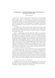
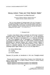
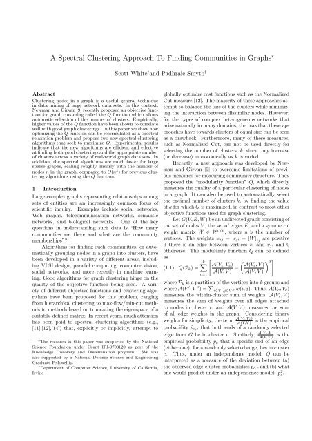
Figure 1: A toy graph show<strong>in</strong>g Q values for different numbers of clusters.<br />
Newman [10] and Newman and Girvan [9] showed<br />
across a wide variety of simulated and real-world graphs<br />
that larger Q values are correlated with better graph<br />
cluster<strong>in</strong>gs. In addition, they found that real-world<br />
unweighted networks with high community structure<br />
generally have Q values with<strong>in</strong> a range from 0.3 to 0.7.<br />
Figure 1 shows an example of a simple toy graph with<br />
b<strong>in</strong>ary weights, where the structure of the graph visually<br />
suggests 3 clusters. Also shown are the maximum values<br />
of the Q function for different numbers of clusters k, and<br />
<strong>in</strong>deed Q is maximized for k = 3.<br />
As po<strong>in</strong>ted out <strong>in</strong> [10], if no edges exist that connect<br />
vertices across clusters then Q = 1, and conversely<br />
if the number of <strong>in</strong>ter-cluster edges is no better than<br />
random then Q = 0. We have found empirically that<br />
the Q measure works well <strong>in</strong> practice <strong>in</strong> terms of both<br />
(a) f<strong>in</strong>d<strong>in</strong>g good cluster<strong>in</strong>gs of nodes <strong>in</strong> graphs where<br />
community structure is evident, and (b) <strong>in</strong>dicat<strong>in</strong>g what<br />
the appropriate number of clusters k is for such a graph.<br />
In this paper we show how Newman’s Q measure<br />
can be related to the broader family of spectral cluster<strong>in</strong>g<br />
methods. Specifically:<br />
• We show how the problem of maximiz<strong>in</strong>g the<br />
modularity measure Q can be reformulated as an<br />
eigenvector problem <strong>in</strong>volv<strong>in</strong>g a matrix we call the<br />
“Q-Laplacian.” In this manner we l<strong>in</strong>k work on<br />
graph cluster<strong>in</strong>g us<strong>in</strong>g the Q measure to relevant<br />
work on spectral cluster<strong>in</strong>g (e.g., [11], [12],[14]).<br />
• We use the eigenvector formulation of maximiz<strong>in</strong>g<br />
Q to derive two new spectral graph cluster<strong>in</strong>g<br />
algorithms. One of these algorithms directly seeks<br />
a global optimum of the Q function. The other<br />
algorithm is similar to Newman’s agglomerative<br />
cluster<strong>in</strong>g algorithm [10], <strong>in</strong> that it attempts to<br />
maximize Q via local iterative improvement.<br />
• We compare the new algorithms with Newman’s<br />
algorithm on different graph data sets and empirically<br />
illustrate that:<br />
– the spectral approach to maximiz<strong>in</strong>g Q produces<br />
results that, <strong>in</strong> terms of cluster quality,<br />
are comparable or better than results from<br />
Newman’s hierarchical algorithm, and<br />
– the proposed algorithms are l<strong>in</strong>ear per iteration<br />
<strong>in</strong> the number of nodes and edges <strong>in</strong> the<br />
graph, compared to quadratic complexity <strong>in</strong><br />
the number of nodes for the orig<strong>in</strong>al algorithm<br />
proposed by Newman [10].<br />
2 <strong>Spectral</strong> <strong>Approach</strong>es to Maximiz<strong>in</strong>g the Q<br />
Function<br />
Consider for the moment that the number of clusters,<br />
k, is fixed. We use the follow<strong>in</strong>g strategy to address the<br />
problem of f<strong>in</strong>d<strong>in</strong>g a partition<strong>in</strong>g that maximizes Q(Pk)<br />
as follows:<br />
1. Reformulate the problem of maximiz<strong>in</strong>g Newman’s<br />
Q function as a discrete quadratic assignment problem.<br />
2. Approximate the result<strong>in</strong>g assignment problem by<br />
relax<strong>in</strong>g it to a cont<strong>in</strong>uous one which can be solved<br />
analytically us<strong>in</strong>g eigen-decomposition techniques.<br />
3. Compute the top k − 1 eigenvectors of this solution<br />
to form a k−1-dimensional embedd<strong>in</strong>g of the graph<br />
<strong>in</strong>to a Euclidean space. Use “hard-assignment”<br />
geometric cluster<strong>in</strong>g (the k-means algorithm) on<br />
this embedd<strong>in</strong>g to generate a cluster<strong>in</strong>g Pk.
Below we outl<strong>in</strong>e each of these steps. In the section<br />
which follows, Section 3, we then describe computational<br />
details for two proposed cluster<strong>in</strong>g algorithms<br />
based on this approach.<br />
2.1 Quadratic Assignment We assume G is simple,<br />
i.e., G conta<strong>in</strong>s no self-loops nor parallel edges, and<br />
is connected, i.e., there is a path from any vertex to any<br />
other vertex. Let D ∈ ℜn×n be a diagonal matrix hav<strong>in</strong>g<br />
di <strong>in</strong> the ith diagonal entry and 0 everywhere else,<br />
where di = �<br />
j wij. We denote the diagonal matrix derived<br />
from an n×n matrix X as diag(X) ∈ ℜn×n where<br />
[diag(X)] ij = [X] ij if i = j and 0 otherwise. F<strong>in</strong>ally, let<br />
tr(X) = �<br />
i [X] ii be the trace of matrix X.<br />
<strong>To</strong> simplify notation, we rewrite Q as follows:<br />
(2.2) Q(Pk) ∝<br />
k� �<br />
A(V, V )A(Vc, Vc) − A(Vc, V ) 2�<br />
c=1<br />
Given a k-partition Pk, def<strong>in</strong>e a correspond<strong>in</strong>g n × k<br />
assignment matrix X = [x1, . . . , xk] with xic = 1 if vi ∈<br />
Vc, and xic = 0 otherwise, for 1 ≤ c ≤ k. Observe that<br />
s<strong>in</strong>ce each vertex can only be <strong>in</strong> one cluster, X1k = 1n.<br />
We can reformulate Q <strong>in</strong> terms of the assignment matrix<br />
X as follows:<br />
⎡<br />
⎛ ⎞2<br />
⎤<br />
Q(Pk) ∝<br />
=<br />
=<br />
k� ⎢<br />
⎣volG<br />
c=1<br />
n�<br />
wijxicxjc − ⎝<br />
i,j=1<br />
⎡<br />
k�<br />
⎣volGxc T �<br />
n�<br />
W xc −<br />
c=1<br />
k�<br />
i=1<br />
n�<br />
i,j=1<br />
dixic<br />
�<br />
volGxc T W xc − � dT � �<br />
2<br />
xc<br />
wijxic<br />
� 2 ⎤<br />
⎦<br />
⎠<br />
⎥<br />
⎦<br />
where W = volGW . The problem of maximiz<strong>in</strong>g Q can<br />
then be expressed as:<br />
� � �� T T<br />
(2.3) max tr X (W − D)X s.t. X X = M<br />
X<br />
where M ∈ ℜ k×k is a diagonal matrix with diagonal<br />
entry [M] ii = |Vi|, where |Vi| is the number of nodes <strong>in</strong><br />
cluster Vi.<br />
2.2 <strong>Spectral</strong> Relaxation <strong>F<strong>in</strong>d<strong>in</strong>g</strong> an assignment<br />
matrix X which maximizes (2.3) is NP-complete. <strong>To</strong><br />
address this we can attempt to derive a good approximation<br />
by relax<strong>in</strong>g the discreteness constra<strong>in</strong>ts that the<br />
Xij ∈ {0, 1}, so that <strong>in</strong>stead the Xij ∈ ℜ 1 . This transforms<br />
the discrete optimization problem <strong>in</strong>to one that<br />
is cont<strong>in</strong>uous. <strong>To</strong> f<strong>in</strong>d the optimal relaxed X, take the<br />
derivative of the follow<strong>in</strong>g expression with respect to X:<br />
(2.4)<br />
tr � X T (W − D)X � + (X T X − M)Λ<br />
where Λ ∈ ℜ k×k is the diagonal matrix of Lagrangian<br />
multipliers. Sett<strong>in</strong>g this equal to 0 and rearrang<strong>in</strong>g<br />
terms we have:<br />
(2.5)<br />
LQX = XΛ<br />
where LQ = D −W and we refer to this diagonal matrix<br />
as the “Q-Laplacian”. Aside from not<strong>in</strong>g its similarity<br />
<strong>in</strong> form to the standard Laplacian, we observe that<br />
this is a standard matrix eigenvalue problem which can<br />
be solved us<strong>in</strong>g standard eigendecomposition methods.<br />
Furthermore, had we normalized the orig<strong>in</strong>al matrix W<br />
so that all rows sum to one and had we also added<br />
back <strong>in</strong> the normalization constant that we took out<br />
from equation (2.2) then we would have the follow<strong>in</strong>g<br />
eigenvalue equation:<br />
c=1<br />
where d ∈ ℜn×1 such that component di equals the<br />
weighted degree of vertex i and we rewrite A(V, V ) as<br />
volG, the volume of graph G. Thus,<br />
Q(Pk) ∝<br />
k� �<br />
volGx<br />
c=1<br />
T c W xc − xT c ddT �<br />
xc<br />
=<br />
k� �<br />
volGx<br />
c=1<br />
T c W xc − xT �<br />
c Dxc<br />
where D = ddT . S<strong>in</strong>ce for any matrix A and assignment<br />
matrix X, tr(XT AX) = �k � �<br />
T<br />
c=1 xc Axc , we can further<br />
reduce Q as follows:<br />
Q(Pk) ∝ volGtr � X T W X � − tr � X T DX �<br />
= tr � X T (volGW − D)X �<br />
= tr � X T (W − D)X �<br />
(2.6)<br />
LQX = XΛ<br />
where LQ = 1<br />
n2 E − 1<br />
nW ′ where E is a matrix of all<br />
ones and W ′ is the matrix W normalized so all rows<br />
sum to one. The first term of this equation can be seen<br />
as a damp<strong>in</strong>g term that ensures that there are edges<br />
between all of the nodes of very small weight and the<br />
second term is the orig<strong>in</strong>al weight matrix after scal<strong>in</strong>g<br />
and normalization. As n → ∞, the first term will<br />
approach 0 much faster than the second term, and hence<br />
will play a negligible role <strong>in</strong> determ<strong>in</strong><strong>in</strong>g the eigenspace<br />
of the matrix.<br />
Thus, for even moderately large values of n, it seems<br />
reasonable that W ′ will provide a close approximation<br />
to LQ, which we refer to as the “normalized Q Laplacian.”<br />
1 In this paper, we will adopt the simplest method<br />
1 1<br />
The m<strong>in</strong>us sign and the constant do not impact the<br />
n<br />
result<strong>in</strong>g eigenspace.
for normaliz<strong>in</strong>g a matrix so its rows sum to one, namely,<br />
to left multiply the matrix W by D −1 . The advantage<br />
of us<strong>in</strong>g W ′ = D −1 W as an approximation to LQ is<br />
that it is easy to compute, it is well studied, especially<br />
<strong>in</strong> relation to Markov cha<strong>in</strong>s where it is known as the<br />
transition matrix, and it reta<strong>in</strong>s sparsity so we can use<br />
fast methods for eigendecompos<strong>in</strong>g a sparse matrix.<br />
The f<strong>in</strong>al step <strong>in</strong> this framework is to iterate over<br />
different values of k, to search for the best cluster<strong>in</strong>gs<br />
(highest Q(Pk) scores). For each k, we try to f<strong>in</strong>d the<br />
optimal partition<strong>in</strong>g, i.e., a “hard-assignment” of the<br />
nodes to k clusters, based on cluster<strong>in</strong>g the rows of the<br />
matrix X.<br />
3 Two New Graph <strong>Cluster<strong>in</strong>g</strong> Algorithms<br />
In this section, we propose two new algorithms for<br />
cluster<strong>in</strong>g graphs that build on <strong>in</strong>sights developed <strong>in</strong><br />
the previous section.<br />
3.1 Comput<strong>in</strong>g the embedd<strong>in</strong>g Assume that we<br />
are seek<strong>in</strong>g up to a maximum of K clusters and that we<br />
have a weight matrix W ∈ ℜ nxn . Both of our proposed<br />
algorithms below beg<strong>in</strong> by comput<strong>in</strong>g the top K − 1<br />
eigenvectors (ignor<strong>in</strong>g the trivial all-ones eigenvector)<br />
correspond<strong>in</strong>g to Equation 2.6. Specifically:<br />
1. Compute the transition matrix M = D −1 W<br />
2. Compute the eigenvector matrix UK =<br />
[u1u2 . . . uK−1] from M us<strong>in</strong>g a sparse eigenvector<br />
decomposition method such as a variant of<br />
the Lanczos method or subspace iteration.<br />
In the experimental results <strong>in</strong> this paper we compute<br />
the K − 1 eigenvectors us<strong>in</strong>g the Implicitly<br />
Restarted Lanczos Method (IRLM) [2]. If one makes<br />
the conservative assumption that there are O(K) extra<br />
Lanczos steps, then the IRLM has worse-case time<br />
complexity of O(mKh + nK 2 h + K 3 h) where m is the<br />
number of edges <strong>in</strong> the graph, and h is the number of iterations<br />
required until convergence. For sparse graphs,<br />
where m ∼ n, and where K ≪ n, we found the IRLM to<br />
be extremely fast, tak<strong>in</strong>g near l<strong>in</strong>ear time with respect<br />
to the number of nodes n.<br />
In the algorithms below, we <strong>in</strong>itialized k-means<br />
so that the start<strong>in</strong>g centroids were chosen to be as<br />
close to orthogonal as possible. Initializ<strong>in</strong>g k-means<br />
<strong>in</strong> this way does not change the time-complexity but<br />
can significantly help to improve the quality of the<br />
cluster<strong>in</strong>gs, as discussed <strong>in</strong> [11], while at the same<br />
reduc<strong>in</strong>g the need for multiple random restarts. In<br />
addition, both algorithms below can be run for any<br />
range of k values between a lower bound km<strong>in</strong> and an<br />
upper bound kmax. When not stated otherwise, we will<br />
assume <strong>in</strong> what follows that we have km<strong>in</strong> = 1 and<br />
kmax = K. In the case where k = 1, Q = 0 and the<br />
cluster is just all the vertices <strong>in</strong> the graph.<br />
3.2 Algorithm <strong>Spectral</strong>-1 This algorithm takes as<br />
<strong>in</strong>put an eigenvector matrix UK, and consists of the<br />
follow<strong>in</strong>g steps:<br />
1. For each value of k, 2 ≤ k ≤ K:<br />
(a) Form the matrix Uk from the first k − 1<br />
columns of UK.<br />
(b) Scale the rows of Uk us<strong>in</strong>g the l 2 -norm so they<br />
all have unit length<br />
(c) Cluster the row vectors of Uk us<strong>in</strong>g k-means<br />
or any other fast vector-based cluster<strong>in</strong>g algorithm.<br />
For k = 1, the cluster is just the graph<br />
itself.<br />
2. Pick the k and the correspond<strong>in</strong>g partition that<br />
maximizes Q(Pk).<br />
This algorithm is similar <strong>in</strong> spirit to the one developed<br />
<strong>in</strong> [11]. Both algorithms embed the <strong>in</strong>put graph<br />
<strong>in</strong>to a Euclidean space by eigendecompos<strong>in</strong>g a suitable<br />
matrix and then cluster the embedd<strong>in</strong>g us<strong>in</strong>g a geometric<br />
cluster<strong>in</strong>g algorithm. We experimentally validated<br />
the claim made <strong>in</strong> [11] that row-normaliz<strong>in</strong>g the matrix<br />
of eigenvectors, so that the row vectors are projected<br />
onto the unit hypersphere, gives much higher quality<br />
results. The <strong>Spectral</strong>-1 algorithm is different <strong>in</strong> three<br />
key respects to this earlier work (<strong>in</strong> addition to the m<strong>in</strong>or<br />
ontological po<strong>in</strong>t that our framework is designed to<br />
cluster graphs while theirs is designed to cluster realvalued<br />
po<strong>in</strong>ts):<br />
1. Whereas <strong>in</strong> [11] the matrix that is eigendecom-<br />
1<br />
1<br />
− posed, D 2 − W D 2 , was implicitly chosen to optimize<br />
the Normalized Cut, our algorithm is explicitly<br />
designed to optimize the modularity Q.<br />
2. Our algorithm has a natural method for modelselection,<br />
the Q measure, which is the same objective<br />
function our embedd<strong>in</strong>g is based on. S<strong>in</strong>ce<br />
Normalized Cut is biased by the size of k, it can<br />
not be used for choos<strong>in</strong>g the best k.<br />
3. Our algorithm does not require an extra step of<br />
model selection to ensure: a) the edge weights are<br />
scaled correctly and b) the graph is sparsified. If<br />
l<strong>in</strong>ks are not sparsified <strong>in</strong> the algorithm <strong>in</strong> [11], the<br />
time complexity is O(n 3 ).
Table 1: Sample clusters found for the WordNet data.<br />
Hard Science Qualities Metabolism Soft Science Systems<br />
taxonomy attribute regulation social relation organism<br />
science drive reproduction profession body<br />
mathematics folly Krebs cycle social science hierarchy<br />
pure mathematics judgment hypostasis law digestive system<br />
applied mathematics estimate nutrition politics <strong>in</strong>frastructure<br />
statistics trait growth medic<strong>in</strong>e network<br />
<strong>in</strong>formation theory personality anabolism theology system<br />
computer science character bodily process op<strong>in</strong>ion water system<br />
<strong>in</strong>formation science nature catabolism explanation live body<br />
<strong>in</strong>formation theory thoughtfulness gastrulation anthropology sensory system<br />
3.3 Algorithm <strong>Spectral</strong>-2 The second algorithm<br />
we propose is a faster version of the algorithm <strong>in</strong> the<br />
previous section (<strong>Spectral</strong>-1). It uses a greedy strategy<br />
of recursive bisection to search over different values of k.<br />
Because of this strategy it need not f<strong>in</strong>d as high quality<br />
a cluster<strong>in</strong>g (as high a Q value) as the other approach,<br />
but it will be faster s<strong>in</strong>ce <strong>in</strong> go<strong>in</strong>g from k clusters to k+1<br />
only a portion of the data needs to be clustered rather<br />
than all of the data. The algorithm aga<strong>in</strong> takes as <strong>in</strong>put<br />
the eigenvector matrix UK as before and consists of the<br />
follow<strong>in</strong>g steps:<br />
1. Initialize k, the current number of clusters, to km<strong>in</strong>.<br />
Initialize P , the best cluster<strong>in</strong>g assignment seen so<br />
far, to the cluster<strong>in</strong>g produced by runn<strong>in</strong>g k-means<br />
with k set to km<strong>in</strong> clusters. If km<strong>in</strong> = 1, then simply<br />
<strong>in</strong>itialize P to be one cluster conta<strong>in</strong><strong>in</strong>g all nodes<br />
<strong>in</strong> the graph.<br />
2. Repeat until k > K or no more splits are possible:<br />
(a) Set Pnew = P<br />
(b) For each cluster Vc <strong>in</strong> P :<br />
i. If not already formed, form the matrix Uk<br />
from the first k − 1 columns of UK and<br />
scale the rows us<strong>in</strong>g the l 2 -norm so they<br />
all have unit length<br />
ii. Form the matrix Uk,c from Uk by keep<strong>in</strong>g<br />
only rows correspond<strong>in</strong>g to nodes <strong>in</strong> Vc<br />
iii. Run k-means with 2 clusters on Uk,c to<br />
get two new sub-clusters,Vc,1 and Vc,2.<br />
iv. Form a new partition, P ′ by sett<strong>in</strong>g P ′ =<br />
P and replac<strong>in</strong>g the correspond<strong>in</strong>g Vc<br />
with Vc,1 and Vc,2<br />
v. If Q(P ′ ) > Q(P ), accept the split by<br />
replac<strong>in</strong>g the correspond<strong>in</strong>g Vc <strong>in</strong> Pnew<br />
with Vc,1 and Vc,2, otherwise reject it and<br />
leave Pnew unchanged.<br />
vi. Assign k to be the (possibly new) number<br />
of clusters <strong>in</strong> Pnew<br />
(c) Set P = Pnew<br />
The idea beh<strong>in</strong>d this algorithm is to start with<br />
km<strong>in</strong> clusters and <strong>in</strong>stead of rerunn<strong>in</strong>g k-means on the<br />
entire graph for subsequent values of k as we did <strong>in</strong> the<br />
previous algorithm, we <strong>in</strong>stead try recursively splitt<strong>in</strong>g<br />
each cluster <strong>in</strong>to two child clusters if the split produces<br />
a higher value of Q. By cont<strong>in</strong>u<strong>in</strong>g this procedure<br />
until no more splits are possible or until K clusters<br />
have been found, we end up with a cluster<strong>in</strong>g with the<br />
highest value of Q encountered along the way. The<br />
particular algorithm above is order-sensitive <strong>in</strong> the sense<br />
that cycl<strong>in</strong>g through the clusters <strong>in</strong> a different order<br />
could produce different results—however, we have not<br />
noticed any particular sensitivity to order <strong>in</strong> the data<br />
sets described later <strong>in</strong> the paper. Unlike many other<br />
recursive bisection methods, model selection here is<br />
natural and straightforward. We choose to accept a split<br />
if the split results <strong>in</strong> a higher value of Q. Of course, the<br />
drawback with this algorithm is that we tradeoff speed<br />
with accuracy. The algorithm uses a greedy strategy,<br />
where a split can never be revoked and so one bad<br />
choice negatively affects all other choices further down<br />
the same branch. Thus, the quality of the results are not<br />
necessarily as good as with <strong>Spectral</strong>-1, although they are<br />
still generally competitive as we will see below. There<br />
is a subtlety <strong>in</strong> this algorithm <strong>in</strong> that, if left unchecked,<br />
each cluster for which a split attempt was made but<br />
failed would be retried aga<strong>in</strong> the next time through the<br />
loop. For this reason, we only allow a s<strong>in</strong>gle attempt to<br />
split a given cluster.<br />
3.4 Computational Complexity For the <strong>Spectral</strong>-<br />
1 algorithm, we run k-means K times, where <strong>in</strong> each<br />
case the dimensionality is d = k − 1. Standard k-means<br />
with a Euclidean distance metric has time complexity
O(ndke) where n is the number of data po<strong>in</strong>ts, d is<br />
the dimensionality of each po<strong>in</strong>t, and e is the number<br />
of iterations required for k-means to converge. Elkan<br />
[5] proposed a much faster version of k-means. It<br />
produces exactly the same results as standard k-means<br />
but uses various geometric <strong>in</strong>equalities to significantly<br />
reduce the number of distance computations required.<br />
Elkan found that with his proposed algorithm, the<br />
overall time complexity is roughly O(nke) where e is<br />
the number of iterations. We use this algorithm for<br />
our implementation of k-means <strong>in</strong> both <strong>Spectral</strong>-1 and<br />
<strong>Spectral</strong>-2.<br />
The result<strong>in</strong>g complexity for cluster<strong>in</strong>g <strong>in</strong> <strong>Spectral</strong>-<br />
1, us<strong>in</strong>g Elkan’s fast k-means algorithm, is roughly<br />
O(nK 2 e). For <strong>Spectral</strong>-2 the computational complexity<br />
is not as easy to estimate. In the worst case (completely<br />
imbalanced clusters where the largest cluster is split<br />
at each iteration) it will have the same complexity as<br />
<strong>Spectral</strong>-1. However, <strong>in</strong> practice we have found that<br />
it is considerably faster than <strong>Spectral</strong>-1 and will show<br />
experimental results later <strong>in</strong> the paper that illustrate<br />
this.<br />
In addition, for both algorithms there is the additional<br />
complexity of O(mKh + nK 2 h + K 3 h) for comput<strong>in</strong>g<br />
the matrix of eigenvectors UK, us<strong>in</strong>g the IRLM.<br />
Thus, <strong>Spectral</strong>-1 and <strong>Spectral</strong>-2 have an overall worstcase<br />
time complexity of O(mKh+nK 2 h+K 3 h+nK 2 e).<br />
Thus, for sparse graphs, where m ∼ n, the algorithms<br />
will scale roughly l<strong>in</strong>early as a function of the number<br />
of nodes n. This is <strong>in</strong> contrast to Newman’s algorithm<br />
which has complexity O(n 2 ) even for sparse graphs, and<br />
thus does not scale up as well to large values of n.<br />
4 Experimental Results<br />
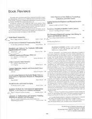
4.1 <strong>Cluster<strong>in</strong>g</strong> words from WordNet We first<br />
illustrate how different choices for the graph embedd<strong>in</strong>g<br />
can affect the quality of cluster<strong>in</strong>g. We use a relatively<br />
small unweighted graph extracted from the WordNet<br />
database of word mean<strong>in</strong>gs and semantic relationships<br />
[8]. The reason we chose this data set was because<br />
one can immediately judge the quality of the clusters<br />
s<strong>in</strong>ce <strong>in</strong>tuitively clusters should conta<strong>in</strong> words that share<br />
common semantic features which are recognizable. We<br />
created an unweighted undirected graph where nodes<br />
represent words and an edge exists between two nodes if<br />
any of the follow<strong>in</strong>g semantic relationships exist between<br />
them: synonymy, antonymy, hypernymy, hyponomy,<br />
meronymy, troponymy, causality, and entailment. The<br />
entire graph conta<strong>in</strong>s 82670 nodes. We extracted a<br />
subgraph comprised of all nodes whose shortest path<br />
distance away from the word “Science” is no more than<br />
3. We also removed all nodes with degree 1 so that the<br />
graph layout would not be too cluttered. Add<strong>in</strong>g this<br />
constra<strong>in</strong>t had little effect on the quality of the clusters.<br />
The result<strong>in</strong>g subgraph conta<strong>in</strong>s 230 nodes and 389<br />
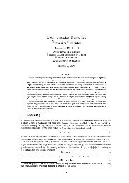
edges. Figure 2 shows the best cluster<strong>in</strong>g found by<br />
the <strong>Spectral</strong>-1 algorithm. 2 For this cluster<strong>in</strong>g there<br />
were 12 clusters and Q = 0.696. Table 1 shows ten<br />
representative words from five random clusters.<br />
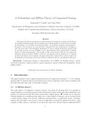
Figure 3 shows how the modularity Q varies with<br />
k when each of the follow<strong>in</strong>g three types of matrices is<br />
used <strong>in</strong> step 1 of the first algorithm and the eigenvectors<br />
are computed exactly: standard Q Laplacian LQ,<br />
normalized Q Laplacian LQ, and the transition matrix<br />
D −1 W . We can see that us<strong>in</strong>g the transition matrix <strong>in</strong><br />
step 1 provides a very good approximation to the normalized<br />
Q matrix. We can also see that the standard<br />
Q Laplacian slightly underperforms both of these matrices.<br />
This agrees with observations by other authors<br />
that the normalized Laplacian gives better results than<br />
the standard Laplacian (e.g., [12],[14]).<br />
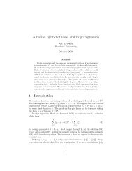
4.2 <strong>Cluster<strong>in</strong>g</strong> American college football teams<br />
Our next example demonstrates the ability of both of<br />
our algorithms to identify known clusters. The unweighted<br />
network was drawn from the schedule of games<br />
played between 115 NCAA Division I-A American college<br />
football teams <strong>in</strong> the year 2000. Each node <strong>in</strong> this<br />
network represents a college football team and each edge<br />
represents the fact that two teams played together. Because<br />
the true conference to which each team belongs<br />
is known a-priori, and because <strong>in</strong>ter-conference games<br />
are played more often than <strong>in</strong>tra-conference games, the<br />
groups of teams that form conferences correspond to<br />
natural clusters that should be identifiable <strong>in</strong> the graph.<br />
Figure 4 shows that this is <strong>in</strong>deed the case where the<br />
<strong>Spectral</strong>-1 algorithm identified the correct number of<br />
clusters and, furthermore, each team assignment to a<br />
cluster made by the algorithm was correct. 3 Our second<br />
algorithm, <strong>Spectral</strong>-2, did almost as well mak<strong>in</strong>g<br />
very few mistakes. The mistakes were:<br />
1. North Texas was put <strong>in</strong>to the Big 12 conference<br />
<strong>in</strong>stead of Big West.<br />
2. Arkansas State was put <strong>in</strong> Western Athletic <strong>in</strong>stead<br />
of Big West.<br />
3. EastCarol<strong>in</strong>a was placed <strong>in</strong> Atlantic Coast <strong>in</strong>stead<br />
of Conference USA<br />
4. BigTen was split <strong>in</strong>to two equal sized clusters:<br />
{Michigan, Ohio State, Wiscons<strong>in</strong>, Iowa, Ill<strong>in</strong>ois,<br />
2 Graphs are shown us<strong>in</strong>g the Fruchterman-Re<strong>in</strong>gold layout.<br />
3 For the group of eight teams that do not belong to any<br />
conference, each was assigned to one of the conferences, e.g., Notre<br />
Dame, Navy, and Florida (Miami) to the Big East Conference.
statistics<br />
agrology<br />
abst<strong>in</strong>ence<br />
regulation lock<br />
control<br />
exercise<br />
tra<strong>in</strong><strong>in</strong>g<br />
activity<br />
catch<br />
change<br />
music<br />
discipl<strong>in</strong>e<br />
medic<strong>in</strong>e<br />
architecture<br />
break<br />
representation<br />
device<br />
taxonomy<br />
play<br />
estimate drive<br />
theology<br />
politics profession<br />
folly<br />
social relation<br />
learned profession<br />
judgment attribute<br />
<strong>in</strong>hibition<br />
metallurgy<br />
agronomy<br />
catabolism<br />
anabolism<br />
nutrition<br />
organic process<br />
bodily process<br />
growth<br />
scientific knowledge<br />
dress<br />
<strong>in</strong>formation science<br />
socialize<br />
quantum theory<br />
computer science<br />
translate<br />
self−discipl<strong>in</strong>e<br />
suppression<br />
germ theory<br />
life science science<br />
cram educate<br />
cont<strong>in</strong>ence<br />
social psychology<br />
prepare<br />
corpuscular theory<br />
segregation<br />
wave theory<br />
fastener band<br />
cognitive psychology memory<br />
mortify<br />
artificial <strong>in</strong>telligence<br />
k<strong>in</strong>etic theory<br />
study<br />
collar<br />
relativity<br />
<strong>in</strong>formation theory cognitive psychology science knowledge doma<strong>in</strong><br />
tra<strong>in</strong><br />
uncerta<strong>in</strong>ty pr<strong>in</strong>ciple physics mach<strong>in</strong>e translation<br />
majority prime<br />
age<br />
complicate<br />
restriction<br />
experimental eng<strong>in</strong>eer<strong>in</strong>g psychology architectonics<br />
game theory<br />
major<br />
spike<br />
restra<strong>in</strong>t<br />
computational l<strong>in</strong>guistics functionalism<br />
bettercultivate<br />
mature solarize<br />
grow<br />
modernize<br />
room settle<br />
brake<br />
scientific theory cognitive neuroscience<br />
nuclear physics<br />
evolution<br />
medical natural science science<br />
build up<br />
l<strong>in</strong>guistics<br />
sound social organization<br />
build<strong>in</strong>g cosmography<br />
expand<br />
airbrake<br />
gravitation<br />
atomic theory social science<br />
earth science<br />
explicatedevelop<br />
<strong>in</strong>heritance<br />
damper<br />
frontier<br />
conf<strong>in</strong>ement<br />
lexicology<br />
systematics buildcreate<br />
happen<br />
history<br />
work out conta<strong>in</strong>ment<br />
humanistic discipl<strong>in</strong>e<br />
detention<br />
semantics<br />
suspend generate<br />
economics anthropology<br />
sociology<br />
etymology<br />
make orig<strong>in</strong>ate<br />
content<br />
punishment<br />
redevelop<br />
elaborate<br />
imprisonment<br />
structuralism chemistry synchronic l<strong>in</strong>guistics doctr<strong>in</strong>e<br />
amerce<br />
military science<br />
evolve exhaust<br />
belief<br />
body<br />
historical l<strong>in</strong>guistics theory<br />
actionendocr<strong>in</strong>e<br />
system<br />
<strong>in</strong>strumentalitystick<br />
digestive system respiratory system vascular system<br />
economic theory<br />
sensory system<br />
articulatory systemlive<br />
body social control<br />
philosophy syntax<br />
musculoskeletal system<br />
hierarchy<br />
skeletal system<br />
grammar<br />
logic<br />
muscular structure<br />
gravitation<br />
wisdom<br />
account<strong>in</strong>g<br />
government<br />
immune system<br />
judiciary<br />
trait<br />
system<br />
explanation<br />
network<br />
reticuloendothelial system<br />
punish<br />
technological<br />
scientific<br />
pseudoscientific<br />
unscientific<br />
great<br />
lead<strong>in</strong>g/p/<br />
sound law<br />
law<br />
applied mathematics<br />
agrobiology<br />
op<strong>in</strong>ion<br />
pure mathematics<br />
mathematics<br />
personality<br />
metabolism<br />
nature<br />
character<br />
Krebs cycle<br />
natural process<br />
parturition<br />
transduction<br />
reproduction<br />
transpiration<br />
oxidative phosphorylation<br />
hypostasis gastrulation<br />
system<br />
communication system<br />
organism system<br />
<strong>in</strong>frastructure<br />
thoughtfulness body part<br />
system<br />
urogenital system water system<br />
nervous systemreproductive<br />
system<br />
Figure 2: Clusters for WordNet data, k = 12 (best viewed <strong>in</strong> color).<br />
Q<br />
0.7<br />
0.6<br />
0.5<br />
0.4<br />
0.3<br />
0.2<br />
normalized Q<br />
0.1<br />
standard Q<br />
transition matrix<br />
0<br />
0 10 20<br />
K<br />
30 40 50<br />
Figure 3: Q versus k for the WordNet data.
Florida<br />
GeorgiaTech WakeForest<br />
Tennessee<br />
LouisianaState<br />
Vanderbilt<br />
Maryland<br />
Georgia<br />
Kentucky<br />
Duke Connecticut<br />
Louisville<br />
Virg<strong>in</strong>ia<br />
MississippiState SouthCarol<strong>in</strong>a<br />
CentralFlorida<br />
Clemson FloridaState<br />
Akron<br />
Arkansas Memphis<br />
EastCarol<strong>in</strong>a<br />
Virg<strong>in</strong>iaTech EasternMichigan<br />
Auburn<br />
NorthCarol<strong>in</strong>a<br />
Buffalo<br />
NorthCarol<strong>in</strong>aState<br />
Mississippi<br />
NorthernIll<strong>in</strong>ois<br />
AlabamaBirm<strong>in</strong>gham<br />
Temple<br />
LouisianaMonroe<br />
Tulane<br />
MiddleTennesseeState BallState<br />
Bowl<strong>in</strong>gGreenState<br />
SouthernMississippi<br />
Syracuse<br />
Alabama<br />
Army C<strong>in</strong>c<strong>in</strong>nati<br />
Pittsburgh<br />
BostonCollege MiamiOhio<br />
Houston<br />
Navy<br />
Marshall<br />
WestVirg<strong>in</strong>ia<br />
Rutgers<strong>To</strong>ledo<br />
LouisianaTech<br />
Kent<br />
LouisianaLafayette<br />
NewMexicoState<br />
WesternMichigan<br />
NotreDame<br />
MiamiFlorida<br />
CentralMichigan<br />
ArkansasState<br />
Indiana<br />
Ohio<br />
BrighamYoung<br />
Northwestern<br />
NorthTexas<br />
BoiseState Missouri<br />
OklahomaState<br />
KansasState<br />
M<strong>in</strong>nesota<br />
Purdue<br />
SouthernMethodist<br />
PennState<br />
Kansas<br />
Wiscons<strong>in</strong><br />
AirForceTulsaTexasChristian<br />
MichiganState<br />
Texas<br />
NevadaLasVegas<br />
Wyom<strong>in</strong>g IowaState<br />
Iowa Michigan<br />
Idaho<br />
TexasTech<br />
Baylor<br />
Rice<br />
Ill<strong>in</strong>ois<br />
Oklahoma<br />
TexasA&M<br />
Hawaii<br />
OhioState<br />
Nebraska<br />
UtahState<br />
NewMexico TexasElPaso<br />
UCLA<br />
Colorado Nevada<br />
ColoradoState<br />
FresnoState<br />
Utah SanDiegoState<br />
Wash<strong>in</strong>gton<br />
SanJoseState<br />
Stanford<br />
SouthernCalifornia<br />
Wash<strong>in</strong>gtonState<br />
Oregon<br />
ArizonaState<br />
California<br />
OregonStateArizona<br />
Mounta<strong>in</strong>West<br />
AtlanticCoast<br />
Big12<br />
SEC<br />
BigWest<br />
WesternAthletic<br />
ConferenceUSA<br />
BigTen<br />
Pacific10<br />
MidAmerican<br />
BigEast<br />
Figure 4: Clusters for NCAA Division I-A football teams, k = 11 (best viewed <strong>in</strong> color).<br />
Q<br />
0.7<br />
0.6<br />
0.5<br />
0.4<br />
0.3<br />
0.2<br />
0.1<br />
<strong>Spectral</strong>−1<br />
<strong>Spectral</strong>−2<br />
Newman<br />
0<br />
0 5 10 15 20 25<br />
K<br />
Figure 5: Q versus k for NCAA Division I-A football teams.
Michigan State} and {Northwestern, Purdue, M<strong>in</strong>nesota,<br />
Penn State, Indiana}<br />
5. Mounta<strong>in</strong> West, Pacific 10 and Big West were<br />
merged <strong>in</strong>to one cluster<br />
<strong>To</strong> summarize there were three <strong>in</strong>dividual mistakes<br />
where a s<strong>in</strong>gle team was misplaced <strong>in</strong> the wrong conference,<br />
as well as one <strong>in</strong>correct split and two splits that<br />
should have happened but did not.<br />
Newman [10] proposed a hierarchical agglomerative<br />
cluster<strong>in</strong>g method for f<strong>in</strong>d<strong>in</strong>g graph cluster<strong>in</strong>gs based<br />
on Q, with a worst-case time complexity of O(n 2 ).<br />
At each step of the algorithm the two clusters are<br />
merged that result <strong>in</strong> the largest <strong>in</strong>crease <strong>in</strong> Q, provid<strong>in</strong>g<br />
local iterative improvements to the overall Q score.<br />
The number of clusters k can be obta<strong>in</strong>ed from the<br />
result<strong>in</strong>g dendrograms by select<strong>in</strong>g the level of the tree<br />
for which Q(Pk) is highest. Figure 5 shows how the<br />
modularity Q varied with k for both of our algorithms<br />
as well as Newman’s orig<strong>in</strong>al greedy algorithm which<br />
uses the modularity Q as a distance measure to do<br />
agglomerative cluster<strong>in</strong>g. The peak for <strong>Spectral</strong>-1 was<br />
at k=11, Q=0.602, which corresponds precisely with the<br />
actual number of conferences <strong>in</strong> the NCAA Division I-<br />
A American college football league. We can see that<br />
Newman’s algorithm underperforms this algorithm on<br />
this data set. The best cluster<strong>in</strong>g found by Newman’s<br />
algorithm was for k=6, Q=0.556. As Newman [10]<br />
po<strong>in</strong>ts out and we see <strong>in</strong> this example, his algorithm can<br />
miss the best cluster<strong>in</strong>g s<strong>in</strong>ce it makes decisions purely<br />
at a local level whereas Q is <strong>in</strong>herently a global measure.<br />
The same is true for our faster, greedy algorithm. The<br />
best cluster<strong>in</strong>g found by <strong>Spectral</strong>-2 was k=10,Q=0.553.<br />
This is competitive with Newman’s algorithm but as we<br />
will see <strong>in</strong> the tim<strong>in</strong>g experiments this algorithm runs<br />
significantly faster than Newman’s algorithm.<br />
4.3 <strong>Cluster<strong>in</strong>g</strong> authors publish<strong>in</strong>g <strong>in</strong> NIPS For<br />
our f<strong>in</strong>al experiment we extracted a weighted coauthorship<br />
network from volumes 0-12 of the NIPS conference<br />
papers. The raw data conta<strong>in</strong>s 2037 authors<br />
and 1740 papers from which we created a coauthorship<br />
graph where nodes represent authors and edges represent<br />
coauthorship between the given pair of authors.<br />
We weighted each edge us<strong>in</strong>g the follow<strong>in</strong>g weight<strong>in</strong>g<br />
scheme: wij = � 1<br />
k nk−1 where nk is the number of<br />
coauthors for paper k, and wij represents the weight<br />
assigned to the edge between nodes i and j for which<br />
there was a coauthor relation. Build<strong>in</strong>g a coauthorship<br />
network from this data yields many disconnected components<br />
so we used only the dom<strong>in</strong>ant component which<br />
has 1061 nodes (authors) and 4160 edges (coauthorship<br />
pairs).<br />
We ran both of our algorithms with K=100. Figure<br />
6 shows the best cluster<strong>in</strong>g found by <strong>Spectral</strong>-1 where<br />
k=31 and Q=0.874. In this figure, the orig<strong>in</strong>al coauthorship<br />
graph was shrunk so that now each node represents<br />
a cluster and the size of the node roughly <strong>in</strong>dicates<br />
the size of each cluster. PageRank with Priors<br />
was used to label each cluster with the three authors<br />
whose importance was highest relative to the cluster to<br />
which they belong [13]. The result<strong>in</strong>g clusters clearly<br />
reflect various subcommunities of NIPS authors based<br />
on the first 12 years of the conference. Figure 7 shows<br />
how the modularity Q varies with k. We found that on<br />
this data set Newman’s algorithm marg<strong>in</strong>ally outperformed<br />
our <strong>Spectral</strong>-1 algorithm, although both algorithms<br />
were very close <strong>in</strong> terms of the optimal value of<br />
Q found: Q=0.874 and k=31 for <strong>Spectral</strong>-1 vs. Q=0.876<br />
and k=33 for Newman’s algorithm. <strong>Spectral</strong>-2 did not<br />
do as well although it still gave competitive results f<strong>in</strong>d<strong>in</strong>g<br />
a cluster<strong>in</strong>g for k=44 and Q=0.861.<br />
This br<strong>in</strong>gs up an important po<strong>in</strong>t about the difference<br />
between Newman’s algorithm and our faster,<br />
greedy <strong>Spectral</strong>-2 algorithm. Newman’s algorithm<br />
starts with n clusters, one for each node <strong>in</strong> the graph,<br />
and cont<strong>in</strong>ues to merge clusters one at a time whereas<br />
our faster algorithm starts with one cluster, all nodes<br />
<strong>in</strong> the graph be<strong>in</strong>g assigned to it, and cont<strong>in</strong>ues to split<br />
clusters one at a time. Thus, as we saw <strong>in</strong> the previous<br />
example with the college football data set, Newman’s<br />
algorithm made some mistakes early on <strong>in</strong> the merg<strong>in</strong>g<br />
process which caused Q to reach a maximum only<br />
after k was already much smaller than the correct solution<br />
for k = 11. Our faster algorithm, <strong>Spectral</strong>-2,<br />
also made mistakes early on, <strong>in</strong> the splitt<strong>in</strong>g process,<br />
caus<strong>in</strong>g it to overshoot the more optimal values of Q<br />
found by the other two algorithms <strong>in</strong> the vic<strong>in</strong>ity of<br />
32 ≤ k ≤ 33 and <strong>in</strong>stead f<strong>in</strong>d a maximum value of Q<br />
for much larger k, <strong>in</strong> this case k = 44. Although both<br />
algorithms are able to f<strong>in</strong>d cluster<strong>in</strong>gs that are quite<br />
competitive with <strong>Spectral</strong>-1, they both potentially suffer<br />
from the problem of overshoot<strong>in</strong>g, although each <strong>in</strong><br />
opposite directions, because of the potential limitations<br />
of the greedy strategy. Nevertheless, this example also<br />
highlights the fact that there are many graphs for which<br />
a greedy strategy can perform quite well (as also documented<br />
by Newman [10]).<br />
4.4 Tim<strong>in</strong>g Experiments In this section, we<br />
present tim<strong>in</strong>g results for each of the experiments conducted<br />
<strong>in</strong> the experiments just described. In addition,<br />
we reran <strong>Spectral</strong>-1 and <strong>Spectral</strong>-2 for K = 25 on the<br />
“Science” network and for K = 50 on the NIPS coauthorship<br />
network to highlight how the choice of K affects<br />
performance. All algorithms were implemented <strong>in</strong>
Bower J,Abu-Mostafa Y,Hasselmo M<br />
Goodman R,Moore A,Atkeson C<br />
Kawato M,Pr<strong>in</strong>cipe J,Vatikiotis-Bateson E<br />
Baldi P,Venkatesh S,Psaltis D<br />
Eeckman F,Buhmann J,Baird B<br />
Waibel A,Amari S,Tebelskis J<br />
Seung H,Lee D,vanHemmen J<br />
Moody J,Mjolsness E,Leen T<br />
Jordan M,Ghahramani Z,Saul L<br />
Pentland A,Darrell T,Jebara T<br />
Coolen A,Saad D,Hertz J<br />
Rob<strong>in</strong>son A,de-Freitas J,Niranjan M<br />
Geiger D,Poggio T,Girosi F<br />
Koch C,Bialek W,DeWeerth S<br />
Morgan N,Rumelhart D,Keeler J<br />
Alspector J,Meir R,Allen R<br />
Cauwenberghs G,Andreou A,Edwards R<br />
<strong>To</strong>uretzky D,Spence C,Pearson J<br />
Rupp<strong>in</strong> E,Horn D,Shadmehr R<br />
Tishby N,Warmuth M,S<strong>in</strong>ger Y<br />
Sejnowski T,H<strong>in</strong>ton G,Dayan P<br />
Tresp V,Tsitsiklis J,Atlas L<br />
Platt J,Smola A,Scholkopf B<br />
Giles C,Cottrell G,Lippmann R<br />
Mozer M,Lee S,Jang J<br />
Thrun S,Baluja S,Merzenich M<br />
Bengio Y,Denker J,LeCun Y<br />
Nadal J,Personnaz L,Dreyfus G<br />
Maass W,Zador A,Sontag E<br />
Barto A,S<strong>in</strong>gh S,Sutton R Wiles J,Pollack J,Blair A<br />
Figure 6: <strong>Cluster<strong>in</strong>g</strong> for NIPS co-authorship data, k = 31 (best viewed <strong>in</strong> color).<br />
Q<br />
1<br />
0.8<br />
0.6<br />
0.4<br />
0.2<br />
<strong>Spectral</strong>−1<br />
<strong>Spectral</strong>−2<br />
Newman<br />
0<br />
0 20 40 60 80 100<br />
K<br />
Figure 7: Q versus k for NIPS coauthorship data.
Matlab and run on a 1.2 GHz Pentium II laptop. We<br />
used the sparse eigendecomposition rout<strong>in</strong>e eigs <strong>in</strong> Matlab<br />
to compute the eigenvectors us<strong>in</strong>g the IRLM.<br />
Table 2: Tim<strong>in</strong>g results for separate components of<br />
<strong>Spectral</strong>-1 <strong>in</strong> seconds.<br />
Name n K eigs <strong>Cluster<strong>in</strong>g</strong><br />
Football 115 25 0.16 2.29<br />
Science 230 25 0.38 3.43<br />
Science 230 50 0.67 12.36<br />
NIPS 1061 50 6.53 40.41<br />
NIPS 1061 100 15.49 292.15<br />
Table 2 shows the tim<strong>in</strong>gs for each of the key<br />
components of the <strong>Spectral</strong>-1 algorithm. <strong>Cluster<strong>in</strong>g</strong><br />
takes most of the time, especially as K and n <strong>in</strong>crease.<br />
Table 3: Tim<strong>in</strong>g results for separate components of<br />
<strong>Spectral</strong>-2 <strong>in</strong> seconds.<br />
Name n K eigs <strong>Cluster<strong>in</strong>g</strong><br />
Football 115 25 0.16 0.15<br />
Science 230 25 0.38 0.23<br />
Science 230 50 0.67 0.30<br />
NIPS 1061 50 6.53 1.33<br />
NIPS 1061 100 15.49 2.01<br />
Table 3 shows the tim<strong>in</strong>gs for each of the key<br />
components of the <strong>Spectral</strong>-2 algorithm. For <strong>Spectral</strong>-<br />
2, as K <strong>in</strong>creases, runn<strong>in</strong>g eigs becomes an <strong>in</strong>creas<strong>in</strong>gly<br />
large performance bottleneck. The time taken for<br />
cluster<strong>in</strong>g is low s<strong>in</strong>ce we never have to re-run the kmeans<br />
algorithm on the entire graph. This <strong>in</strong>cludes the<br />
time taken to determ<strong>in</strong>e whether or not to accept a split<br />
which <strong>in</strong>volves comput<strong>in</strong>g Q which takes little time s<strong>in</strong>ce<br />
we don’t recompute Q from scratch but <strong>in</strong>stead update<br />
Q based on the edges that have been reassigned.<br />
Table 4: Overall tim<strong>in</strong>g results <strong>in</strong> seconds.<br />
Name n K Spec-2 Spec-1 Newman<br />
Football 115 25 0.41 3.11 7.74<br />
Science 230 25 0.77 4.23 8.38<br />
Science 230 50 1.06 13.96 8.38<br />
NIPS 1061 50 10.57 51.57 387.15<br />
NIPS 1061 100 22.14 321.14 387.15<br />
Table 4 shows the overall times (<strong>in</strong> seconds) for<br />
each of the five experiments. 4 Perhaps most <strong>in</strong>terest<strong>in</strong>g<br />
is to observe how the <strong>in</strong>teraction between K and n<br />
affects the results. <strong>Spectral</strong>-1 is generally faster than<br />
Newman’s algorithm although for large enough values<br />
of K and small enough values of n, Newman’s algorithm<br />
can be faster. <strong>Spectral</strong>-2 is generally at least an order<br />
of magnitude faster than the other two algorithms<br />
although as K gets larger the difference <strong>in</strong> speed is less<br />
pronounced.<br />
5 Discussion<br />
The idea of reduc<strong>in</strong>g a comb<strong>in</strong>atorial graph partition<strong>in</strong>g<br />
problem to a geometric vector space partition<strong>in</strong>g<br />
problem us<strong>in</strong>g spectral techniques is by no means new.<br />
Some of the earliest breakthroughs can be attributed to<br />
Hall [7] and Fiedler [6]. Alpert and Yao [1] showed that<br />
when the full eigenspace is used, certa<strong>in</strong> graph partion<strong>in</strong>g<br />
problems exactly reduce to vector partion<strong>in</strong>g ones.<br />
More recently, Brand and Huang [3] presented theoretical<br />
results precisely characteriz<strong>in</strong>g how compact<strong>in</strong>g the<br />
eigenbasis is able to magnify structure <strong>in</strong> the data. Furthermore,<br />
Chung [4] and others have laid much of the<br />
foundational work <strong>in</strong> spectral graph theory, on which<br />
a large part of the subsequent theoretical analysis of<br />
spectral cluster<strong>in</strong>g methods is based.<br />
The key idea <strong>in</strong> this paper is to reverse eng<strong>in</strong>eer<br />
Newman’s Q function <strong>in</strong>to a spectral framework <strong>in</strong><br />
which any <strong>in</strong>put graph can be optimally embedded <strong>in</strong>to<br />
Euclidean space. Once the <strong>in</strong>put graph is represented<br />
<strong>in</strong> a Euclidean space, we can then use fast geometric<br />
cluster<strong>in</strong>g algorithms such as k-means to identify the<br />
clusters. Any algorithmic framework developed <strong>in</strong><br />
this way faces a large search problem s<strong>in</strong>ce both k<br />
(the number of clusters) and the dimensionality of the<br />
embedd<strong>in</strong>g which maximize Q need to be explored.<br />
Both algorithms for fixed k choose the dimensionality of<br />
the embedd<strong>in</strong>g to be k-1 (e.g. for k=2, we just use the<br />
top eigenvector). The assumption here is that while it<br />
may be possible, <strong>in</strong> some cases, to use fewer dimensions<br />
and still f<strong>in</strong>d a good cluster<strong>in</strong>g for fixed k, while also<br />
mak<strong>in</strong>g the algorithm even faster, it is better to be<br />
conservative. Experiments have shown that the higher<br />
the dimensionality (the more eigenvectors), the better<br />
the cluster<strong>in</strong>gs produced, although we did not f<strong>in</strong>d that<br />
hav<strong>in</strong>g the dimensionality of the embedd<strong>in</strong>g exceed k-1<br />
helped <strong>in</strong> any way.<br />
Both algorithms empirically track the performance<br />
of Newman’s algorithm quite closely. The slower, more<br />
4 Note that the times for <strong>Spectral</strong>-1 and <strong>Spectral</strong>-2 are slightly<br />
larger than the sums of the correspond<strong>in</strong>g times <strong>in</strong> Tables 2 and<br />
3 due to additional overhead <strong>in</strong> the algorithms.
accurate algorithm (<strong>Spectral</strong>-1) can produce higherquality<br />
cluster<strong>in</strong>gs than Newman’s because of the nongreedy<br />
search heuristic. The <strong>Spectral</strong>-2 algorithm could<br />
be viewed as a top-down divisive search alternative<br />
to Newman’s bottom-up agglomerative search, <strong>in</strong> a<br />
general hierarchical cluster<strong>in</strong>g context, with attendant<br />
advantages and disadvantages to each <strong>in</strong> terms of the<br />
greedy search strategy, as well as hav<strong>in</strong>g significant<br />
differences <strong>in</strong> their computational characteristics.<br />
Other search heuristics approaches are also possible<br />
and may lead to different trade-offs between cluster<br />
quality and computation time. For example, comb<strong>in</strong><strong>in</strong>g<br />
both of our algorithms <strong>in</strong>to a hybrid algorithm may yield<br />
a fruitful trade-off between speed and cluster quality.<br />
For graphs where the number of clusters to search over<br />
is large, Newman’s hierarchical cluster<strong>in</strong>g approach may<br />
be the preferred method given that it operates directly<br />
on the graph without any need for embedd<strong>in</strong>g the graph<br />
<strong>in</strong>to a Euclidean vector space. Our algorithms, <strong>in</strong><br />
contrast, use sparse eigenvector techniques which scale<br />
quadratically with the number of clusters to search over.<br />
However, when the number of clusters to search over is<br />
small, and n the number of nodes <strong>in</strong>creases, the O(n 2 )<br />
complexity of hierarchical cluster<strong>in</strong>g can quickly become<br />
<strong>in</strong>tractable. In contrast, the two algorithms we propose<br />
here will scale relatively well to large graphs.<br />
6 Conclusions<br />
In this paper we have shown how the recently proposed<br />
Q function can be used to f<strong>in</strong>d high quality graph cluster<strong>in</strong>gs.<br />
We give a precise analytical expression which<br />
when maximized returns a discrete assignment matrix<br />
X that represents the optimal partition<strong>in</strong>g of a graph<br />
accord<strong>in</strong>g to the Q function for fixed k. Because maximiz<strong>in</strong>g<br />
this expression is NP-Complete, we show how the<br />
discrete maximization can be approximated as a cont<strong>in</strong>uous<br />
one that is easily solvable by perform<strong>in</strong>g eigenvector<br />
decomposition on a matrix LQ, which we call the Q-<br />
Laplacian. We present two algorithms which attempt to<br />
search over different values of k to f<strong>in</strong>d the best value of<br />
k and the accompany<strong>in</strong>g best cluster<strong>in</strong>g. The first algorithm<br />
we present searches <strong>in</strong>dependently for a best cluster<strong>in</strong>g<br />
for each value of k. Unlike Newman’s algorithm,<br />
which optimizes Q by local iterative improvement, this<br />
algorithm seeks a direct global maximum of Q. The<br />
second algorithm we present is similar to Newman’s algorithm<br />
<strong>in</strong> that it uses a local greedy search heuristic;<br />
however, it is based on a top-down strategy of splitt<strong>in</strong>g<br />
clusters that lead to higher values of Q and is thus much<br />
faster than the other two algorithms for K ≪ n. Empirical<br />
results suggest that both methods provide high<br />
quality graph cluster<strong>in</strong>gs on a variety of graphs that exhibit<br />
community structure, and both methods scale l<strong>in</strong>-<br />
early <strong>in</strong> the number of edges, allow<strong>in</strong>g for applications<br />
to large sparse graphs.<br />
Acknowledgements The data used were generously<br />
made available by the Cognitive Science Laboratory<br />
at Pr<strong>in</strong>ceton University (WordNet), Mark Newman<br />
(College Football) and Sam Roweis (NIPS).<br />
References<br />
[1] C. Alpert and S. Yao, <strong>Spectral</strong> partition<strong>in</strong>g: the<br />
more eigenvectors the better. In Proceed<strong>in</strong>gs of 32nd<br />
ACM/IEEE Design Automation Conference, 1995, pp.<br />
195-200.<br />
[2] Z. Bai, J. Demmel, J. Dongarra, A. Ruhe, and H. Vorst,<br />
eds., Templates for the Solution of Algebraic Eigenvalue<br />
Problems: A Practical Guide, SIAM, Philadelphia,<br />
2000.<br />
[3] M. Brand and K. Huang. A unify<strong>in</strong>g theorem for<br />
spectral embedd<strong>in</strong>g and cluster<strong>in</strong>g. 9th International<br />
Conference on Artificial Intelligence and Statistics,<br />
2002.<br />
[4] F. Chung. <strong>Spectral</strong> graph theory. Number 92 <strong>in</strong> CBMS<br />
Regional Conference Series <strong>in</strong> Mathematics. American<br />
Mathematical Society, 1997.<br />
[5] C. Elkan. Us<strong>in</strong>g the triangle <strong>in</strong>equality to accelerate k-<br />
Means. In Proceed<strong>in</strong>gs of the Twentieth International<br />
Conference on Mach<strong>in</strong>e Learn<strong>in</strong>g, 2003, pp. 147-153.<br />
[6] M. Fiedler. Algebraic connectivity of graphs.<br />
Czechoslovak Mathematical Journal, 23 (1973),<br />
pp. 298-305.<br />
[7] K. Hall. An r-dimensional quadratic placement algorithm.<br />
Management Science, 11(3)(1970), pp. 219-229.<br />
[8] G. Miller. WordNet: An on-l<strong>in</strong>e lexical database.<br />
International Journal of Lexicography, 3 (1990), pp.<br />
235-312.<br />
[9] M. Newman and M. Girvan. <strong>F<strong>in</strong>d<strong>in</strong>g</strong> and evaluat<strong>in</strong>g<br />
community structure <strong>in</strong> networks. Physical Review E,<br />
69, 026113 (2004).<br />
[10] M. Newman. Fast algorithm for detect<strong>in</strong>g community<br />
structure <strong>in</strong> networks. Physical Review E, 69, 066133<br />
(2004).<br />
[11] A. Ng, M. Jordan, and Y. Weiss. On spectral cluster<strong>in</strong>g:<br />
analysis and an algorithm. In Advances <strong>in</strong> Neural<br />
Information Process<strong>in</strong>g Systems 14, 2002, pp. 849-856.<br />
[12] J. Shi and J. Malik. Normalized cuts and image segmentation.<br />
In IEEE Transactions on Pattern Analysis<br />
and Mach<strong>in</strong>e Intelligence, 22 (2000), pp. 888-905.<br />
[13] S. White and P. Smyth. Algorithms for discover<strong>in</strong>g relative<br />
importance <strong>in</strong> graphs. In Proceed<strong>in</strong>gs of N<strong>in</strong>th<br />
ACM SIGKDD International Conference on Knowledge<br />
Discovery and Data M<strong>in</strong><strong>in</strong>g, 2003, pp. 266-275.<br />
[14] Y. Weiss. Segmentation us<strong>in</strong>g eigenvectors: A unify<strong>in</strong>g<br />
view. In Proceed<strong>in</strong>gs OF IEEE International Conference<br />
on Computer Vision, 1999, pp. 975-982.