- Page 2:
This page intentionally left blank
- Page 8:
THE DYNAMICS OFCOASTAL MODELSCliffo
- Page 12:
ContentsPrefacepage ixAcknowledgeme
- Page 16:
Contentsvii9 Aspects of stratificat
- Page 22:
xPrefacethe word model, ormodeling,
- Page 36:
Geomorphic classification of ocean
- Page 40:
Geomorphic classification of ocean
- Page 44:
Geomorphic classification of ocean
- Page 48:
Geomorphic classification of ocean
- Page 52:
Distinctive features of coastal bas
- Page 56:
Distinctive features of coastal bas
- Page 60:
Distinctive features of coastal bas
- Page 64:
Distinctive features of coastal bas
- Page 68:
Distinctive features of coastal bas
- Page 72:
Distinctive features of coastal bas
- Page 76:
Types of model 23is a distinction b
- Page 80:
Types of model 251.4.3 Theory or mo
- Page 84:
Types of model 27a system and analy
- Page 88:
Terminology in the sciences of wate
- Page 92:
Further reading 311.6 Further readi
- Page 96:
Position of a point 33horizontal pl
- Page 100:
Velocities 35Whatever method is use
- Page 104:
Velocities 37the vertical velocity
- Page 108:
NFluxes 39San FranciscoLosAngelesTo
- Page 112:
Two-dimensional models 41fluxes mul
- Page 116:
Volume continuity equation 43zH inu
- Page 120:
Volume continuity equation 45dxw (z
- Page 124:
Sources and sinks 47either grow in
- Page 128:
Sources and sinks 490.2y0.10−3
- Page 132:
functions, such as a surface wind s
- Page 136:
Linearized continuity equation 53wh
- Page 140:
Potential flow 55In coastal basins
- Page 144:
It follows that we can derive V fro
- Page 148:
Potential flow 59contours of the re
- Page 152:
Conformal mapping 61If S is imagina
- Page 156:
Conformal mapping 63Figure 2.12 Pot
- Page 160:
Conformal mapping 65Figure 2.13 Pot
- Page 164:
3Box and one-dimensional models3.1
- Page 168:
Examples of box models 69Volume exc
- Page 172:
quantity) and S and V are zero orde
- Page 176:
Examples of box models 73If R varie
- Page 180:
Examples of box models 75Table 3.2.
- Page 184:
Examples of box models 77evaporatio
- Page 188:
Examples of box models 79Table 3.5.
- Page 192:
This V tidal comes from the ocean a
- Page 196:
Examples of box models 83Table 3.6.
- Page 200:
Examples of box models 85QheatingT
- Page 204:
derivative of F s with respect to x
- Page 208:
One-dimensional models 89Table 3.8.
- Page 212:
One-dimensional models 913.4.2 Rive
- Page 216:
40Simple models of chemical and bio
- Page 220:
Simple models of chemical and biolo
- Page 224:
This type of box model of ecologica
- Page 228:
Simple models of chemical and biolo
- Page 232:
Further reading 1011Nutrient concen
- Page 236:
Pressure 103@u@t þ u @u ¼ F1 þ F
- Page 240:
Pressure 105Note that ( z) is the h
- Page 244:
Pressure 107We shall attempt to fin
- Page 248:
Pressure 1090z/ h−0.5values of kh
- Page 252:
Pressure 11110.500 10 20Figure 4.3
- Page 256:
Shear stress 113speed at which the
- Page 260:
Shear stress 115shear stress, we sh
- Page 264:
Oscillators 117and repeating this p
- Page 268:
Oscillators 11910 2 Relative an gul
- Page 272:
Oscillators 121Table 4.1. Matlab co
- Page 276:
Oscillators 1231.511.51y0.50y0.50-0
- Page 280:
Effects of a rotating Earth 125110.
- Page 284:
Effects of a rotating Earth 127cfcc
- Page 288:
Effects of a rotating Earth 129for
- Page 292:
Effects of a rotating Earth 13167 m
- Page 296:
Effects of a rotating Earth 133the
- Page 300:
Effects of a rotating Earth 135rota
- Page 304:
Effects of a rotating Earth 137of t
- Page 308:
5Simple hydrodynamic models5.1 Wind
- Page 312:
Wind blowing over irrotational basi
- Page 316:
Wind blowing over irrotational basi
- Page 320:
Wind blowing over irrotational basi
- Page 324:
Wind blowing over irrotational basi
- Page 328:
Wind blowing over irrotational basi
- Page 332:
Wind blowing over irrotational basi
- Page 336:
Wind blowing over irrotational basi
- Page 340:
Ekman balance 1550wind stress−1y
- Page 344:
Ekman balance 1570y-10r = 0.1r = 0.
- Page 348:
Ekman balance 159z 0 zL E(5:41)whe
- Page 352:
Ekman balance 161and using the defi
- Page 356:
Ekman balance 163110.50.5windstress
- Page 360:
Ekman balance 165wind, and as f inc
- Page 364:
Geostrophic balance 167cIncreasingp
- Page 368:
Geostrophic balance 169300y (km)200
- Page 372:
Geostrophic balance 171300y (km)200
- Page 376:
Isostatic equilibrium 173dispersal
- Page 380:
Further reading 175and this is call
- Page 384:
Astronomical tides 177slowly damp t
- Page 388:
Astronomical tides 179can be estima
- Page 392:
Astronomical tides 181Table 6.1. As
- Page 396:
Astronomical tides 183Table 6.3. Ob
- Page 400:
Astronomical tides 185If we add (6.
- Page 404:
Long waves 187initial condition). T
- Page 408:
One-dimensional hydrodynamic models
- Page 412:
One-dimensional hydrodynamic models
- Page 416:
One-dimensional hydrodynamic models
- Page 420:
One-dimensional hydrodynamic models
- Page 424:
One-dimensional hydrodynamic models
- Page 428:
One-dimensional hydrodynamic models
- Page 432:
One-dimensional hydrodynamic models
- Page 436:
Two-dimensional models 203and so as
- Page 440:
Two-dimensional models 205u facevfu
- Page 444:
Two-dimensional models 207(b)100y0.
- Page 448:
Two-dimensional models 2091−50−
- Page 452:
Two-dimensional models 211212019181
- Page 456:
Two-dimensional models 213Table 6.1
- Page 460:
Model speed and the cube rule 215ac
- Page 464:
Model speed and the cube rule 217wh
- Page 468:
Horizontal grids 219Figure 6.21 A g
- Page 472:
Horizontal grids 221field region in
- Page 476:
Vertical structure of model grids 2
- Page 480:
Vertical structure of model grids 2
- Page 484:
Further reading 2276.9 Further read
- Page 488:
Theory of mixing 229mixing or in th
- Page 492:
Theory of mixing 231initial height
- Page 496:
Theory of mixing 233Let us write th
- Page 500:
Theory of mixing 235Table 7.1. Nota
- Page 504:
Theory of mixing 237be the seasonal
- Page 508:
Theory of mixing 239stratified. Str
- Page 512:
Theory of mixing 2410surfacewindwin
- Page 516:
Theory of mixing 243that w e decrea
- Page 520:
Theory of mixing 245i.e., replace t
- Page 524:
For a non-stratified water column i
- Page 528:
Mixing processes and spatial scale
- Page 532: Mixing processes and spatial scale
- Page 536: Mixing processes and spatial scale
- Page 540: The logarithmic layer 255momentum p
- Page 544: The logarithmic layer 257(b)u (m s
- Page 548: The logarithmic layer 259(constant
- Page 552: The logarithmic layer 2610.5100u (m
- Page 556: The logarithmic layer 263and so (7.
- Page 560: 7.8 Friction and energy7.8.1 Energy
- Page 564: Friction and energy 267whereF ð h
- Page 568: Turbulence closure 269that interrel
- Page 572: Dispersion in coastal basins 271qua
- Page 576: Dispersion in coastal basins 273whe
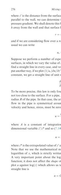
- Page 580: The logarithmic boundary layer 275A
- Page 586: 278 Mixing in coastal basins15linea
- Page 590: 280 Mixing in coastal basinsor~B s
- Page 594: 282 Mixing in coastal basinsand so
- Page 598: 284 Mixing in coastal basinswhere C
- Page 602: 8Advection of momentum8.1 Introduct
- Page 606: (a) (b)flagpoleflashing lightorange
- Page 610: 290 Advection of momentumcurrent (m
- Page 614: 292 Advection of momentumprovided t
- Page 618: 294 Advection of momentum8.2.6 Drog
- Page 622: 296 Advection of momentumFor a typi
- Page 626: tidal channel298 Advection of momen
- Page 630: 300 Advection of momentumTable 8.1.
- Page 634:
302 Advection of momentum0alongshor
- Page 638:
304 Advection of momentumIt essenti
- Page 642:
306 Advection of momentumthrough ti
- Page 646:
308 Advection of momentumbasin, is
- Page 650:
310 Advection of momentumso that by
- Page 654:
312 Advection of momentum3R = 10F <
- Page 658:
314 Advection of momentumThe bottom
- Page 662:
316 Advection of momentumR= 1.5;
- Page 666:
318 Advection of momentumBottom slo
- Page 670:
9Aspects of stratification9.1 Solar
- Page 674:
322 Aspects of stratificationpresen
- Page 678:
324 Aspects of stratificationKineti
- Page 682:
326 Aspects of stratification 1 @ @
- Page 686:
328 Aspects of stratificationT 1 T
- Page 690:
330 Aspects of stratificationand th
- Page 694:
332 Aspects of stratification9.2.1
- Page 698:
334 Aspects of stratificationeither
- Page 702:
336 Aspects of stratification(9.53)
- Page 706:
338 Aspects of stratification0.1G00
- Page 710:
340 Aspects of stratification0Az Ð
- Page 714:
342 Aspects of stratificationTable
- Page 718:
344 Aspects of stratificationwind s
- Page 722:
(a) (b)(c) (d)Figure 9.7 The dotted
- Page 726:
348 Aspects of stratificationcan ch
- Page 730:
BBBBBBBBB350 Dynamics of partially
- Page 734:
352 Dynamics of partially mixed bas
- Page 738:
354 Dynamics of partially mixed bas
- Page 742:
356 Dynamics of partially mixed bas
- Page 746:
358 Dynamics of partially mixed bas
- Page 750:
360 Dynamics of partially mixed bas
- Page 754:
362 Dynamics of partially mixed bas
- Page 758:
364 Dynamics of partially mixed bas
- Page 762:
366 Dynamics of partially mixed bas
- Page 766:
368 Dynamics of partially mixed bas
- Page 770:
370 Dynamics of partially mixed bas
- Page 774:
372 Dynamics of partially mixed bas
- Page 778:
374 Dynamics of partially mixed bas
- Page 782:
376 Dynamics of partially mixed bas
- Page 786:
378 Dynamics of partially mixed bas
- Page 790:
380 Dynamics of partially mixed bas
- Page 794:
382 Dynamics of partially mixed bas
- Page 798:
384 Dynamics of partially mixed bas
- Page 802:
386 Dynamics of partially mixed bas
- Page 806:
388 Dynamics of partially mixed bas
- Page 810:
390 Dynamics of partially mixed bas
- Page 814:
392 Dynamics of partially mixed bas
- Page 818:
11Roughness in coastal basins11.1 I
- Page 822:
396 Roughness in coastal basinscomp
- Page 826:
398 Roughness in coastal basins4.5A
- Page 830:
400 Roughness in coastal basinsof c
- Page 834:
402 Roughness in coastal basins1005
- Page 838:
404 Roughness in coastal basinswher
- Page 842:
406 Roughness in coastal basinsout
- Page 846:
408 Roughness in coastal basinsmari
- Page 850:
410 Roughness in coastal basinsGulf
- Page 854:
412 Roughness in coastal basinsstru
- Page 858:
414 Roughness in coastal basinswher
- Page 862:
416 Roughness in coastal basinsTabl
- Page 866:
418 Roughness in coastal basins0.02
- Page 870:
420 Roughness in coastal basins0.5p
- Page 874:
422 Roughness in coastal basinswave
- Page 878:
424 Roughness in coastal basinsThe
- Page 882:
426 Roughness in coastal basinsTabl
- Page 886:
0.050.050.03TKETKESε S ε0.03TKE (
- Page 890:
N430 Roughness in coastal basinsO A
- Page 894:
432 Roughness in coastal basinsFigu
- Page 898:
434 Roughness in coastal basinscurr
- Page 902:
12Wave and sediment dynamics12.1 In
- Page 906:
438 Wave and sediment dynamics0.04s
- Page 910:
440 Wave and sediment dynamicsthe s
- Page 914:
442 Wave and sediment dynamicsSigni
- Page 918:
444 Wave and sediment dynamicsTable
- Page 922:
446 Wave and sediment dynamics10001
- Page 926:
448 Wave and sediment dynamicsmoved
- Page 930:
450 Wave and sediment dynamicsLet u
- Page 934:
452 Wave and sediment dynamicsTable
- Page 938:
454 Wave and sediment dynamicscumul
- Page 942:
456 Wave and sediment dynamicsHence
- Page 946:
458 Wave and sediment dynamics12.5.
- Page 950:
460 Wave and sediment dynamics100be
- Page 954:
462 Wave and sediment dynamicssuspe
- Page 958:
464 Wave and sediment dynamicsand (
- Page 962:
466 Wave and sediment dynamics10 6
- Page 966:
468 Wave and sediment dynamics wwc
- Page 970:
470 Wave and sediment dynamicsJulie
- Page 974:
472 ReferencesHatcher, B. G. (1990)
- Page 978:
474 ReferencesWhitehead, J. A. (199
- Page 982:
476 Indexbasin (cont.)neutralone-di
- Page 986:
478 Indexdensity (cont.)fronts in b
- Page 990:
480 IndexFram 156Fredsøe, Jørgen
- Page 994:
482 IndexLagrange, Joseph L. 287Lag
- Page 998:
484 Indexphase plane (cont.)node 38
- Page 1002:
486 Indexsidereal day 130sigmacoord
- Page 1006:
488 Indexviscosity (cont.)near awal