TORA Example: Cascade- and Passivity-Based Control Designs ...

292 IEEE TRANSACTIONS ON CONTROL SYSTEMS TECHNOLOGY, VOL. 4, NO. 3, MAY 1996
A Example: Cascade- and Passivity-Based Control Designs
Abstract-We consider the problem of feedback stabilization of
translational oscillations by a rotational actuator (TORA) system.
The main obstacle to controller design is nonlinear coupling from
the rotational to the translational motion through a sinusoidal
term. We present several controller designs based on the cascade
and passivity paradigms.
Mrdjan Jankovic, Dan Fontaine, and Petar V. KokotoviC
I. INTRODUCTION
N this paper we consider the problem of controlling trans-
lational oscillations with a rotational actuator (TORA),
brought to our attention by Bernstein [1], [2]. The motivation
comes from possible use of rotational actuation to remove
some limitations of the current proof-mass actuators. The
problem is also of interest as a case study in nonlinear con-
troller design because the model exhibits nonlinear interaction
between the translational and rotational motions.
The control laws designed in this paper are of two types:
cascade controllers and feedback passivating controllers. Their
properties are illustrated with simulations.
11. TORA SYSTEM MODEL
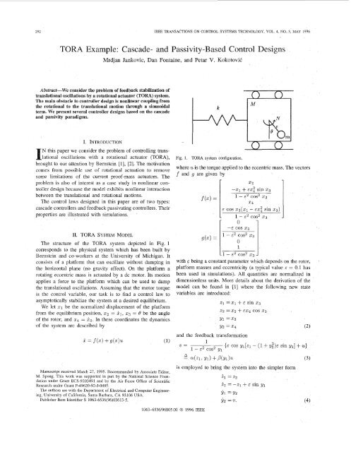
The structure of the TORA system depicted in Fig. 1
corresponds to the physical system which has been built by
Bernstein and co-workers at the University of Michigan. It
consists of a platform that can oscillate without damping in
the horizontal plane (no gravity effect). On the platform a
rotating eccentric mass is actuated by a dc motor. Its motion
applies a force to the platform which can be used to damp
the translational oscillations. Assuming that the motor torque
is the control variable, our task is to find a control law to
asymptotically stabilize the system at a desired equilibrium.
We let 21 be the normalized displacement of the platform
from the equilibrium position, 22 = &I, 23 = 0 be the angle
of the rotor, and 24 = 23. In these coordinates the dynamics
of the system are described by
Manuscript received March 27, 1995 Recommended by Associate Editor,
M Spong This work was supported in part by the National Science Foun-
dation under Grant ECS-9203491 and by the Air Force Office of Scientific
Research under Grant F-49620-92-J-0495
The authors are with the Department of Electrical and Computer Engineer-
ing, University of California, Santa Barbara, CA 93106 USA
Publisher Item Identifier S 1063-6536(96)03613-5
1063-6536/96$05.00 0 1996 IEEE
Fig. 1. ToRA system configuration.
where U is the torque applied to the eccentric mass. The vectors
f and g are given by
I -51
1 -E cos
O X? l
1 - E2 cos2 53
dxc) =
0
1
11 - E2 cos2 53 1
with E being a constant parameter which depends on the rotor,
platform masses and eccentricity (a typical value E = 0.1 has
been used in simulations). All quantities are normalized in
dimensionless units. More details about the derivation of the
model can be found in [1] where the following new state
variables are introduced:
52
+ EX; sin 23 1 - E2 cos2 53
54
z1 = 21 + E sin 2 3
z2 = 5 2 + EX4 cos 23
Y1 =53
Y2 =54
and the feedback transformation
a
= 421, Y1) + P(Yl)U
is employed to bring the system into the simpler form
Zl =z2
Zz = -21 + E sin y1
1
(3)
Yl =y2
y, ='U (4)

IEEE TRANSACTIONS ON CONTROL SYSTEMS TECHNOLOGY, VOL. 4, NO. 3, MAY 1996
Because E is always smaller than one, the transformation from
U to w is nonsingular.
111. CASCADE SYSTEM DESIGNS
stable. One such control law is y1 = - arctan (~0.~2)
Recognizing that y1 is not the control variable, and that the
deviation from its desired value is

294
-1
I v. I
0 5 1 0 1 5 2 0 2 5 3 0 3 5 4 0 4 5 5 0
Normelizod Pmsltw
41 I
Normalized Torque
Fig. 2. Transient behavior with (Cl) and (C2) control laws.
In other words, for some choices of the parameters, the two
control laws would result in the same performance.
Indeed, simulations have shown that the two control laws
are similar even beyond the limiting case. In Fig. 2 the plots'
of translational displacement x1 and the control effort U with
(C1) (solid curve, S = 0) and with (C2) (dashed curve, 6 =
10) show a slight improvement with the backstepping method.
For a clearer illustration of some properties of the backstep-
ping control we consider the following example:
x = -x + g(x)y
y =u.
Since with y G 0 the z-subsystem is globally asymptotically
stable, in the second step of backstepping we let the Lyapunov
function be
Po 2 Pl 2
v=--2 +-y.
2 2
Its derivative along the trajectories of (8) is
V = -Pox2 + Poxg(z)Y + PlYU
and a choice of U which makes V negative definite is
PO
U = -- xg(x) - ay.
P1
With this backstepping control the resulting closed-loop sys-
tem is
This system has the form of a damped nonlinear oscillator. In
contrast, a (C1)-type controller for (8) is simply U = -ay and
results in the closed-loop system which is upper triangular.
Some of the benefits of the term -(po/pl) g(x) introduced by
backstepping are:
1) If, for example, g(x) = x2 a (Cl)-type controller cannot
guarantee global stability. This advantage is not present
in the TORA system which is globally Lipschitz.
'All our plots show 51 and U. To compare them with [l] and [2] the values
shown should be divided by 10
IEEE TRANSACTIONS ON CONTROL SYSTEMS TECHNOLOGY, VOL. 4, NO. 3, MAY 1996
2) When g(z) is globally Lipschitz, or even constant, say
g(z) = go, then -(po/pl)g(z) improves the transient
by reducing the overshoot of x due to an initial condition
of y. If (po/p1) is very small the overshoot is large and,
vice-versa, if (po/pl) is large the overshoot is small.
For the TORA problem this improvement is negligible
because the connection between the two subsystems is
weak (E = 0.1).
IV. FEEDBACK PASSIVATING DESIGNS
The cascade designs in Section I11 resulted in complicated
control laws that require full state feedback and cancellation
of nonlinearities. Our more ambitious design objective is to
use a reduced set of measurements and avoid cancellation of
nonlinearities. This will simplify instrumentation and improve
robustness.
A design paradigm which can be used to accomplish this
objective is feedback passivation [6]. We design three passi-
vating controllers: (Pl), (P2), and (P3). Our basic passivating
feedback controller (Pl) employs a reduced number of states
(zl, y1, y2), but still cancels two nonlinear terms. To avoid
cancellation, we refine the storage function and design the
(P2) controller which has a surprisingly simple form U =
-klyl - k2y2 aad accomplishes our design objective. To
increase the damping of x1 beyond a limit imposed by the
simple structure of (P2), we employ a storage function with
increased penalty on z1 and 22. The resulting passivating
controller (P3) achieves improved damping of 21. It matches
the damping obtained with the cascade control laws, but with
smaller control effort.
We rewrite the TORA system in the (2, y)-coordinates with
the original input U
z1 =22
22 = -21 + E sin y1
$1 =y2
$2 = 421, Y1) + P(Yl)U (9)
with QI and p defined in (2).
(PI) Controller-Feedback Passivation: The (P1)-design
illustrates the feedback passivation procedureJ Its basis is the
requirement that, for a system to be passive from an input U
to an output y = h(x), the relative degree one and weakly
minimum phase conditions must be satisfied.
Choice of the Output Function: For the system (9) the constraint
of relative degree one means that the output h(z, y)
must be a function of y~. So, we let h(z, y) = y ~. With this
output the corresponding zero dynamics subsystem
2.2 = -21 + E sin y1
y, =o (10)
is stable by inspection. This means that the system (9) with
the output y = y2 is weakly minimum phase.

IEEE TRANSACTIONS ON CONTROL SYSTEMS TECHNOLOGY, VOL. 4, NO. 3, MAY 1996 295
Lyapunov Function for the Zero Dynamics: In this step we
want to find a Lyapunov function U(z, yl) for (9) which will
be incorporated into the passivating feedback law. Because y1
is constant, we can treat (10) as a linear system and select
+ - 22” + - y1
1 1
U(Z, y1) = - (21 - E sin ~ 1 ) ~ k1 (11)
2 2 2
with kl being a design parameter. The time derivative of U
along the trajectories of the system (10) is nonpositive, in fact
U = 0, which is satisfactory, since (10) is not asymptotically
stable.
Passivating Feedback and Storage Function: Note that the
system (9) is already in the normal form as defined in [6].
Therefore, the feedback transformation
2 2
= E y2 sin y1 cos y1 - cos2 yl(z1 - E sin yl)
- (1 - E2 cos2 y1)(k1y1 - u1) (12)
renders the system passive from the input u1 to the output y2
with respect to the storage function
-
1 1 k l 2 1 2
W(z, y) = - (21 - E sin y~)’ + - 22” + -yl + - y2. (13)
2 2 2 2
Indeed, E = y2ul which means that the system (9), (12) is
not only passive, but also lossless (see [6] and [7]).
A fundamental passivity property [8], [9] is that the feed-
back connection of a passive and a strictly passive block is
stable in the sense that y2 E L2. Therefore, we can select
any strictly passive feedback control law. The simplest one
is u1 = -k2y2 with which we complete our (Pl) controller
design. Returning to the original control U, (P1) controller is
2 2 3 2
U =E y2 sin y1 cos y1 - E cos yl(z1 - E sin y1)
- (1 - E2 cos2 Yl)(klYl + k2Y2). (PI)
Its passivity property guarantees only stability. Additional
properties are needed to conclude asymptotic stability.
(P2) Controller-Passivation without Cancellation: Even
though it is simpler than (Cl) or (C2), the controller (Pl) has
not completely satisfied the design objective because it uses
three states for feedback and cancels nonlinearities. We now
show that, by modifying the storage function (13) as
1 1 2 h 2
~ ( z y) , = - (21 - E sin ~ 1 + ) - z2 ~ + - y1
2 2 2
y;(1 - E2 cos2 y1) (14)
+ ;
we can achieve the desired objective. The passivating feedback
transformation with respect to W is U = -klyl + u1.
This simple feedback achieves passivity from u1 to yy~ since
I/t’(z, Y) = YZUl.
The next step is to achieve global asymptotic stability.
We close the feedback loop with the simplest strictly passive
block: u1 = -k2y2. Thus our (P2) controller is
U = -k1y1 - k2y2.
(P2)
With the control law (P2) we have = -k2y$ 5 0 which
implies that the origin of the closed-loop system (9), (P2) is
05
= l o
0 5 1 0 1 5 2 0 2 5 3 0 3 5 4 0 4 J M
Nwm(rl/zed b mon
-0.5
0 5 1 0 1 5 2 0 2 5 3 0 3 5 4 0 4 5 5 0
Normdized Torque
Fig. 3. Response of the (P2)-system
stable in the sense of Lyapunov and all the states are bounded.
Because W is radially unbounded these properties are global.
Now we employ LaSalle’s invariance principle to prove
asymptotic stability. The largest invariant set of the closedloop
system (9), (P2) contained in the set R = ((2, y) E
R4: y2 = 0}, where = 0, is determined from y2 0, i.e.,
0 E cos yl(x1 - E sin y1) - klyl.
(15)
Because ~1 = y2 = 0, yl = const. Then it follows from (15)
that z1 = const =+ 22 0 j 22 = z1 - E sin y1 G 0. So the
only solution of (15) inside the set 0 is z1 = y1 = 0 which
proves the global asymptotic stability of z1 = z2 = y1 = y2 =
0.
A typical response of the (P2)-system is shown in Fig. 3
with ICl = 1, k2 = 0.14 chosen for the fastest possible
convergence.
We remark that (P2) controller is a linear version of the
“passive absorber” proposed in [2]. and the plots in Fig. 3
closely resemble those obtained in [2].
The (P2) controller achieves our design objectives because it
does not cancel nonlinearities and uses only the rotor variables
y1 and y2 for feedback. The simulations show that its control
effort is smaller than with (Cl) and (C2). A drawback of
(P2), however, is that the speed of convergence of x1 to zero
cannot be increased by adjusting the gains. This problem will
be resolved by our (P3) controller in the next section. But first
we illustrate some of the possibilities of achieving different
control objectives with simple (P2)-type control laws.
(P2) with Bounded Control: Here we design a control law
which achieves global asymptotic stabilization with the norm
of the input never exceeding some prescribed value 6 > 0.
One such control law is
with k1 < 6. The magnitude of the input Ub is obviously
bounded by 6 and global asymptotic stability follows from the
Lyapunov function

296 IEEE TRANSACTIONS ON CONTROL SYSTEMS TECHNOLOGY, VOL. 4, NO. 3, MAY 1996
'-it
0.5
-1 -5 I 15 2 1
-52 -15 -1 -05 0 05 1
Reel Axis
Fig. 4. Root locus for s2 + bs + a as b varies from 0-00.
Note that we have substituted the quadratic term by a term with
linear growth at infinity. Nevertheless, Wb is positive definite,
radially unbounded and Wb = -(S - k1)y~ arctan y2 5 0.
Again, by LaSalle' s invariance principle, the origin is globally
asymptotically stable.
(P2) with Prespec$ed Equilibrium Structure: We may
want to preserve the existing equilibria or to create a set
of new ones (for example, to prevent unwinding). As an
illustration we use the feedback to create the set of equilibria
at (0, 0, 2kn, 0) with k = 0, fl, f2, .... These equilibria
will necessarily be alternatively stable and unstable. This
objective is achieved by the bounded control
U, = -IC1 sin (0.5~1) - kz arctan yz. (18)
The Lyapunov function is
IC1 2
W, = W - - y1 + 4kl sin2 (0.25~~)
2
(19)
and the invariant set is given by (0, 0, 2kn, 0). It can be
shown that the states converge to one of these equilibria which
represent the same point in physical space.
(P3) Controller-Transient Performance: It has already
been pointed out that the (P2) controller cannot decrease
the settling time of z1 beyond a limit. To explain the reasons
for this limitation and to motivate our approach to overcome
it, we consider the following simple linear system:
This system is passive from the input U to the output y with
respect to the storage function V = (a/2)z2 + iy'. Now
the simplest feedback law which achieves global asymptotic
stability is U = -by which corresponds to the (P2) control for
the system (9).
The root locus for the characteristic equation of the closed-
loop system, as b varies from 0 to 00 and a = 1, is given
in Fig. 4.
It shows that the settling time for z cannot be decreased
arbitrarily.
-1
0 5 10 15 20 25 30 35 40 45 50
Normalized Poshon
4: 5 io 1; 20 25 do j, io 4'5 5L
Normalired Torque
Fig. 5. Response with (P3) and (C2) controllers
To assign a smaller settling time we have to use the z
variable in the feedback law. In the framework of passivating
designs this can be accomplished by modifying the storage
function to increase the penalty on z. Thus with the storage
function V = (a + c/2)z2 + y2, the resulting control law
U = -ex - by achieves arbitrarily small settling time of z by
increasing b and C.
Motivated by the above example we introduce a design
parameter ko to increase the penalty on the z-variables in the
Lyapunov function (14)
ko + 1 kl 2
Wu = ___ [(zl - E sin y1)' + z,2] +
2
+ $ yi(1 - E2 cos2 y1).
The function W, can be made a storage function by the
passivating feedback transformation U = - ~ O E cos yl(-zl +
E. sin y1) - Sly1 SUI. Therefore, our (P3) controller achieving
Wu = < - 0 is given by
U = -he cos yl(-zl + E sin y1) - klyl - kzy2 (~3)
and LaSalle's invariance principle again guarantees that the
origin is globally asymptotically stable. Note that when ko =
0 this control law reduces to (P2).
This design modification significantly improves the settling
time, compared with the (P2) controller. By increasing
the parameter ko we can match the performance of
the cascade controllers, but with smaller control effort as
illustrated in Fig. 5. The solid curves represent the (P3) con-
troller with (ko, k ~ k , ~ = ) (10, 1, 0.5) and the dashed curves
represent the (C2) controller with (PO, PI, pa, CO, cl, CZ) =
(2, 0.2, 1, 2.3, 0.6, 0.6).
Remark 4.1: Note that the controllers (P2) and (P3) guar-
antee global asymptotic stability of the closed-loop system for
any positive values of the gains ko, kl, k ~ Therefore, . if we
multiply the control U by any positive constant, the resulting
control law still achieves global asymptotic stability; in other
words, these controllers have infinite gain margin.
From (2) we have that XI - E sin y1 = 51. Recall that
z1 is the normalized displacement of the platform. If we
\
y1

IEEE TRANSACTIONS ON CONTROL SYSTEMS TECHNOLOGY, VOL. 4, NO. 3, MAY 1996 291
denote by q1 the actual (measured) displacement and by 0
the normalizing factor, we can rewrite (P3) as
Thus, even when E and 0 are not known (i.e., when the mass
parameters of the system are not known), (P3) achieves global
asymptotic stability.
V. CONCLUSION
In this paper we have considered the problem of asymptotic
stabilization of the TORA system. Based on two different
paradigms we have designed several controllers which achieve
global asymptotic stability. Performance of these controllers
was compared by simulations. The summary of our findings
is given below:
For the TORA system the (C2) controller and the much
simpler (Cl) controller give almost the same performance
because the coupling between subsystems is weak.
The (P2) controller uses only 8 and 6 for feedback and
requires the smallest control effort. Its drawback is that
the settling time cannot be decreased beyond a certain
limit.
The (P3) controller allows a faster and better damped
response at the expense of increased control effort and
the addition of a sensor for platform displacement. Still,
the control effort is smaller than with the comparable
cascade controllers.
The design of passivating controllers is not systematic
because it relies on the knowledge of a storage function.
On the other hand, the controller design for cascade
systems is systematic.
ACKNOWLEDGMENT
The authors would like to thank D. S. Bernstein for many
useful discussions and for bringing this control design problem
to their attention.
REFERENCES
[l] C.-J. Wan, D. S. Bernstein, and V. T. Coppola, “Global stabilization
of the oscillating eccentric rotor,” in Proc. 33rd IEEE Con$ Decision
Contr., Dec. 1994, pp. 402444029.
[2] R. T. Bupp, C.-J. Wan, V. T. Cappola, and D. S. Bernstein, “Design of
a rotational actuator for global stabilization of translational motion,” in
Proc. Symp. Active Contr. Vibration Noise, ASME Winter Mtg., 1994.
[3] A. Saberi, P. V. KokotoviC, and H. J. Sussmann, “Global stabilization of
partially linear composite systems,” SIAM J. Contr. Optimization, vol.
28, no. 6, pp. 1491-1503, 1990.
[4] H. J. Sussmann and P. V. KokotoviC, “The peaking phenomenon and
the global stabilization of nonlinear systems,” IEEE Trans. Automat.
Contr., vol. 36, pp. 4244440, 1991.
[5] H. J. Sussmann, E. D. Sontag, and Y. Yang, “A general result on the
stabilization of linear systems using bounded controls,” IEEE Trans.
Automat. Contr., vol. 39, pp. 2411-2425, Dec. 1994.
[6] C. I. Byrnes, A. Isidori, and J. C. Willems, “Passivity, feedback
equivalence, and the global stabilization of minimum phase systems,”
IEEE Trans. Automat. Contr., vol. 36, pp. 1228-1240, Nov. 1991.
171 J. C. Willems, “Dissipative dynamical systems, Part I: General theory,”
Arch. Rational Mech. Anal., vol. 45, pp. 321-351, 1972.
[8] C. A. Desoer and M. Vidyasagar, Feedback Systems: Input-Output
Properties. New York: Academic, 1975.
[9] V. M. Popov, Hyperstability of Control Systems. New York: Springer-
Verlag, 1973.